International Conference on Machine Learning and Computational Intelligence-2017
International Journal of Scientific Research in Computer Science, Engineering and Information Technology © 2017 IJSRCSEIT | Volume 2 | Issue 7 | ISSN : 2456-3307
Problems and Testing the Assumptions of Linear Regression: a
Machine Learning Perspective
Ayoosh Kathuria, Baij Nath Kaushik
Shri Mata Vaishno Devi University, Kakryal, Katra, J&K, India ABSTRACT
Linear Regression is perhaps one of most well-known algorithms in statistics and Machine Learning. Despite its widespread use in machine learning applications, the importance of testing the assumptions of linear regression is often trivialised in machine learning literature. However, the predictions of linear regressions cannot be trusted unless its assumptions are met. An attempt has been made to attract the attention of the community towards this understated aspect of putting linear regression into practice. This paper serves as an endeavour to shed some light on ways to test the assumptions of linear regressions and how to remedy the violations if there are any.
Keywords : Time Series Prediction, Regression Analysis, Linear Regression, Machine Learning
I.
INTRODUCTIONLinear Regression is often the very first algorithm to be taught in any machine learning curriculum. The algorithm, which is borrowed from statistics models the variable we are trying to predict (called the target variable) as a weighted linear combination of one or more inputs variables. Despite its simplicity, it has been deployed across a vast array of real life problems including forecasting stock market trends [1], weather forecasting [2], analysis of automobile engine performance [3], optimising targeted advertising [4] to name a few. The vanilla version of algorithm works by minimising the least squares function, and the performance is judged by the value of the Pearsons coefficient of correlation [5], also referred to as R-squared value (Adjusted R-square for model having multiple input variables. In this paper, whenever we come across the term R-squared, it is to be understood we mean adjusted R-squared in case of multiple input variables)
However, most of the machine learning practitioners often focus on squeezing as much predictive power as they can out of a model, and are often less concerned about the explanatory power of the features used as input. It is also to be noted that the predictions of the model can be trusted only if the assumptions of algorithm are satisfied. In case they are violated, the evaluation metrics, however stellar they might be, are no guarantee for the effectiveness of the model. Hence, it is absolutely fundamental that these assumptions should be rigorously tested while evaluating the performance of Linear Regression. Though these techniques are well documented in statistics literature [6], their coverage in machine learning literature leaves much to be desired.
the reader appreciate why the assumptions are so crucial to the assessment of the model. Second, we perform ordinary least squares regression on Google Stock data from the past ten years. Third, we explore ways to test for the violations of the assumptions and how to fix them. Fourth, we will apply these techniques to fix the violations made by our model and contrast the performance of the new models with the previous one. Finally, we put forth our concluding remarks, and explore the options of using methods other than Linear Regression (LR).
II.
THEORETICAL FRAMEWORKGiven training examples (X, Y), LR tries to establish a
linear relationship between the inputs x(i) ∈ X and
their corresponding labels (value of target variable) y(i)
∈ Y such that
y(i) = θTx(i) + ε(i) (1)
where θ is the weights vector that parametrises the
model, and ε(i) is the error term that captures either
the unmodelled effects (such as features pertinent to predicting target variable that we failed to include in our model), or random noise.
Assumptions of Linear Regression
1) There exists a linear relationship between target
variable and each of the input variables. The
constant variance against time, the target variable as well as the input variables.
3) The errors, ε(i)s are independent and identically
The above equation represents the probability density
of an arbitrary y(i) given a x(i) and is parametrised by θ.
This function, called the likelihood function, depends on θ. We then move to choose a value of θ that maximises the value of this function. This will give us a model that agrees best to our training data.
The joint probability density for the training set can be simply written as the product of probability densities of each training examples, as we have assumed them to be IID (assumption 2). Since we have assumed errors exhibit homoscedasticity, all of
them share a common variance σ2
The likelihood function for the training set could then be written as
(4)
(5) Taking log on both sides of (5) and simplifying it can be shown that maximising likelihood is same as minimising the equation.
(6) This is the standard least squares loss function we minimise during training in LR. The objective of the above treatment was to show how assumptions of LR factor into derivation of the loss function.
Predicting Google’s stock price
where we will use LR for predicting the stock price of Google using the data from the past 10 years. Our goal is to predict the closing price of the stock. The data has been acquired from Quandl, an online platform that hosts financial data. The input features include opening price (Open), highest price (High), lowest price (Low), Closing Price (Close), Volume Traded (Volume), Ex-Dividend, Split Ratio, Adj. Open, Adj. High, Adj. Low, Adj. Close, Adj. Volume collected 10 days prior to the day for which the prediction has to be made. The adjusted ones account for stock splits (One stock becomes two, and the
We are going to limit the feature selection process to dropping all but one amongst the sets of highly correlated features, though feature selection forms
one of the most critical parts of the model training process, we are not going to dwell too much on it here for sake of focusing on the main topic of the paper.
Table 1. Correlation Matrix For Input Features
Open High Low Close Volume
By looking at Table 1 we can clearly see Open, High, Low, Close are highly correlated. Let us drop all of them but Close variable while training our model. We have also dropped Volume to keep things simple in accordance to the principle of Occam’s Razor. We will test another model later which has Volume later in the paper.
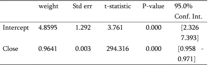
This model achieves a Adj. R-squared of 0.966. A lot of ML practitioners may take it as a conclusive proof of the high efficiency of the model. However, we could also look at the 95.0% Conf. Int or the confidence Intervals for the weights. These are the values which a particular weight may take about 95 out of every 100 times we randomly sample the data from a population and fit the model to it. One should be alarmed if zero also falls in the confidence interval of a weight. This could suggest that there’s a
Since we’re using 95% confidence intervals, the p-value for all the coefficients must be less than 0.05 [7]. We could also look at the T-statistic, which measures the number of standard deviations a weight distribution’s mean is away from zero. Typically, for 95% confidence intervals, T-value should be more than 2 in magnitude. The current model fulfils all the above criteria. High value of R-square, all the p-values below 0.05, and all the t-p-values above 2.
At this point the reader might be edging towards concluding the model does a very good job generalising to the dataset. However, we now proceed to check whether the assumptions of LR are violated or not.
Testing the assumptions of LR Assumption of Linearity
The very premise of testing this assumption can be a tricky bargain. Assuming that there is indeed a linear relationship between the target and the input variable forms the core of our belief that LR is a suitable choice to solve the problem at hand. If we are willing to test this assumption, it means we are ready to consider the case where a linear relationship might not hold, which in turn renders this complete analysis redundant. One might even think that this assumption is merely a leap of faith. However, in practical cases, such assumptions are often backed by domain expertise and guiding principles like the Occams razor.
In fact, a lot of ML practitioners believe a good measure of whether this assumption holds is the R-squared itself. However, R-R-squared is merely the percentage of the target variable variation that is explained by the straight line we have fit. It only describes how well are the input and the target variables correlated. It does not confirm a causal relationship between the target variable and the input variables. Thus, R-squared cannot be solely use to establish our assumption. R-squared simply tells us
the quality of the linear relationship, assuming a linear relationship does exist.
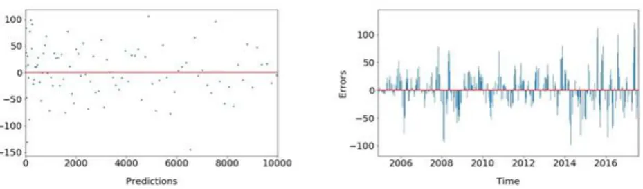
Figure 1. Errors v/s Predicted Values plot for the Google Stock price Model with only Close as the
input variable
Figure 2. Errors v/s Predicted Values plot for a LR model with only x as the input variable. The dataset has a non-linear (quadratic) relationship between the
inputs and the labels, described by y=x2+10x
How to diagnose: Non-linearity can be detected by plotting errors vs the predicted values of the target variable. Figure 1 shows the error v/s predicted values plot for our model.
To get a better insight let us use LR on a dataset having a non-linear (quadratic) relationship between
the input and the target variable, described by y = x2 +
10x. Figure 2 shows
Figure 3. Predicted values v/s errors for a LR model
with x and x2 as the input variables. The dataset has a
non-linear (quadratic) relationship between the
inputs and the labels, described by y=x2+10x
what the Errors v/s Predicted Values plot looks like when we fit a LR model to the dataset.
Remedy: The very first thing one can do is try to apply a non-linear transformation to one or more variables to linearise the relationship. For example, if the target variable is an exponential function of the inputs, applying log transformation to the input variables will linearise the relationship. If a small percentage changes in one or more input variables induces a proportionate percentage change in value of the target variable, the relationship between the inputs and the target variable is a multiplicative one. In such case, a log transformation may be applied to a both the input and the target variables.
One can also try to add another input variable which is simply a non-linear transformation of one of the input variables used in the model. However, such methods could often lead to overfitting, and reguarisation must be used appropriately. One can also come up with a new variable that is a combination (for example, product) of two or more input features used in the model. The cusp of engineering a new input variable to to account for any unmodelled effects.
Assumption of homoscedasticity
This assumption can be tested by looking at the plots of errors vs the predicted value of the target variable, as well as the errors v/s time plot, shown in figure 4 in case of a time series data. By looking at figure 1, we can easily conclude that this assumption is violated as the errors do not have a constant variance across different values of the predicted variable. In particular, the variance seems to increase as the predicted value of the target variable increases.
Again, the violation of this assumption is very evident as we observe the errors do not exhibit a uniform variance.
Figure 4. Errors v/s Time plot for the Google Stock Price Model with only Close as the input variable
Remedy: If the target variable can take only positive values and variance of the errors increases, probably proportionately, as the predicted value of the target variable increases, applying a log transformation to the target variable may stabilise the variance of the
Table 3. Model Evaluation Metrics
Lag 1 2 3
Autocorrelation 0.973 0.946 0.920
consequence of fixing those problems.
In case of time-series data, one may also note a periodic trend in the variances of errors. The variance of errors maybe roughly uniform for periodic intervals. Such a problem may be solved by introducing an additional variable in our model that accounts for seasonal patterns. It maybe also the case the we deal with larger values for some of our input variables in some particular part of the season
resulting in errors of larger magnitude. In that case too, applying a log transformation to target variable can help solve the issue.
Assumptions of Independence
This assumption can be tested by the use of a errors v/s time plot, shown in figure 4. This assumption is clearly violated in plot shown in figure 4. We conclude this by observing that positive errors are followed by positive errors, and negative errors are followed by negative ones for long intervals. This idea can be captured more formally by a mathematical quantity called autocorrelation.
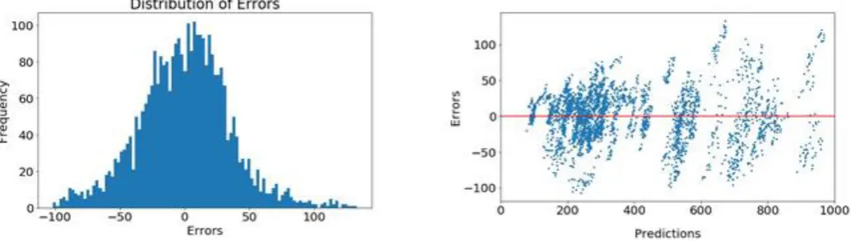
Figure 5. Error histogram for the Google Stock Price Model with only Close as the input variable
Autocorrelation is basically the serial correlation between the errors separated by a fixed amount of time interval (called the lag). The autocorrelations for
most lags should fall between , where n is
the size of the training set. (0.035 for our model). The autocorrelation for errors of our model are given in the table are shown in table 3. This assumption of LR is clearly violated as autocorrelations of our model are away above the threshold that must be adhered to.
Remedy: Mild cases of autocorrelation maybe addressed by adding a time-lagged version of either the target or one of the input variables. If there’s significant autocorrelation at the lag n, one can use a variable lagged by n time intervals to address the issue. There might be seasonal autocorrelation in time series data, wherein errors belonging to the same
season may be correlated. A seasonally lagged variable can be added to the model to address this issue.
Assumption of Normality
This assumption can be simply tested by plotting a histogram of errors. The histogram of errors of our models are shown in figure 5 The reader can see the distribution is not perfectly normal, and seems a bit negatively skewed. Violations of this assumptions arise to due to non-linearity, or the presence of outliers.
question of keeping them in the training dataset or not. To resolve that issue, we must ask ourselves whether they denote merely a statistical fluke or do they represent rare phenomenon which could repeat itself in future.
Figure 6. Predicted v/s Error plot for model having Close and Volume as input variables
5. Fixing violations of assumptions in Google Stock Data Model
Our model fares well on the assumption of linearity as we observe the errors are randomly distributed about the zero mean line in figure 1. However, we had omitted the Volume input variable in our model. We could try a model having Volume as an additional input variable to see if we can get better results on the linearity front. The errors v/s predictions graph is plotted in figure 6. We see no considerable improvements and hence, we stick with our earlier model in spirit of keeping the model simple.
As seen in figure 1 and 4, the assumption of homoscedasticity is clearly violated. In figure 1, we see
Figure 7. Error vs Time plot for model with Close as input and logged target variable
that the variance of errors increases as the value of the stock price increases. It maybe also noted a similar trend is noted in figure 4, where the variance grows as we progress through time (It can be observed that the stock price has risen as we proceed through time too). Such a violation suggests errors are consistent in percentage rather than absolute value. As suggested, earlier we apply a log transformation to our target variable. Figure 7 shows the errors v/s time plot,
Figure 8. Error vs Time plot for model with logged Close as input and logged target variable
which shows improved homoscedasticity of errors in general except a bunch errors of higher variance in the beginning.
Interestingly, it’s a practical observation that stock prices grow with almost constant percentages over
input induces a proportionate percentage change in target variable. Figure 8 shows the error-vs-time plot which exhibits improved homoscedasticity with lesser autocorrelation (still alarmingly high). So, we ditch earlier model for this one now.
Table 4. Model Evaluation Metrics
Lag 1 2 3
Autocorrelation 0.008 -0.003
-0.019
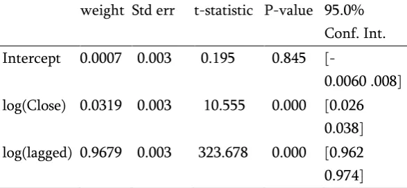
Autocorrelation is still a big problem with our models. One of the ways to fix autocorrelation is to add a lagged variable of our target function (Note, that now we’re referring to a model where we have logged both the target and the input variables). The reader might have noted that the only input variable in our model is Closed is nothing but the value of our target value ten days prior to the day for which we want to make our prediction. However, it is advisable to
arrest autocorrelation at the smallest lag as possible in order to prevent it from percolating to higher lags as well. We find significant autocorrelation at lag 1, and thus add a variable, which is nothing but the target variable lagged by one day. When we plot the Error vs time graph, as shown in the figure 9, we see that the auto-correlation has significantly improved. This fact is confirmed by the autocorrelation figures shown in Table 4.
Figure 9. Error v/s Time plot for model with logged Close and 1-lagged target variable as input and logged target variable
We plot an error histogram in figure 10, and the normality assumption is much more appropriately satisfied than figure 5. As mentioned earlier, the assumption of normality, if violated, is often remedied as a by-product of addressing the other violations. The evaluation metrics for our current model are listed in Table 5
Table 5. Model Evaluation Metrics
weight Std err t-statistic P-value 95.0%
Conf. Int.
Intercept 0.0007 0.003 0.195 0.845
[-0.0060 .008]
log(Close) 0.0319 0.003 10.555 0.000 [0.026
0.038]
log(lagged) 0.9679 0.003 323.678 0.000 [0.962
Figure 10. Error histogram for model with logged Close and 1-lagged target variable as input and logged
target variable
III.
CONCLUSION
So far, we have built a LR model that gives stellar results on the standard evaluation metrics. However, as we tested our model for violations of assumptions of LR, we found that assumptions of homescedasticity and independence were seriously violated. The assumption of normality was also violated to a lesser extent. We then applied appropriate steps to address the issues.
It may be noted that even though we came up with a model that agrees with the assumptions, the results are far from perfect. In fact, there are a couple of anomalies observed throughout our graphs that need to be addressed. We see that even after applying remedying the violations, we observe errors of very high variance in the beginning of the 10-year period, where the value of the stock price was relatively small. We also see high variance around 2008, which can be attributed to sudden steep dip in stock prices owing to the 2008 financial prices.
These anomalies may simply be outliers that may be removed from the data. But we must ask ourselves whether the outliers simply represent statistical flukes or some rare phenomenon that should be accounted for nonetheless. An example is the possibility of a financial crisis happening like one happened in 2008. The crisis was bought about by the liquidity in USA housing market, and therefore it more or less becomes a matter of domain expertise in deciding what our input features should be. It must be noted that the purpose of our analysis was not to build a high quality model, but merely to demonstrate how violations of assumptions of LR can be detected and fixed.
Finally, we may even conclude that perhaps LR may not be the best method to attack the problem. For example, there are many intricacies of modelling stock markets that are far beyond the capabilities of LR. Stock markets are often prone to periods of high and low volatility. This might be the very reason we see high variances in the beginning. This is normal and is often addressed by using ARCH (auto-regressive conditional heteroscedasticity) models wherein the error variance is fitted by an autoregressive model [8].
One of the great difficulties with modelling Stock prices with LR happens to be related to the assumption of independence. In the derivation of the loss function, we assumed our training examples are IID. However, that is quite not the case in real life. A stock’s price on a particular day may be effected by its performance during previous days or months. In such a case, one might think of applying a model which takes into account the effect of the previous values of the target variable into consideration while trying to model its current value. Recurrent Neural Networks are one such example and have shown immensely better results when used for this task [9]
However, this does not discount the value of LR as a valuable modelling tool in any way. The simplicity of LR helps it dodge the curse of overfitting [10] which is one of the biggest problems while training a model in machine learning. Even if one can get past the problem of overfitting in complex models, they can often lack the explanatory power of LR. For instance, while using non-linear regression, we can no longer calculate p-values, and confidence intervals are not guaranteed to be calculable, making it hard to interpret the explanatory power of input variables. Even if LR is not well-suited to attack the problem, it can give us valuable insights which may be used later while testing complex models.
We would also like to thank Sumanta Sarathi Sharma, DoPC, Shri Mata Vaishno Devi University for his valuable insights that greatly helped improve the manuscript.
V.
REFERENCES
[1].T. H. B. Farhad Soleimanian Gharehchopogh and
S. R. Khaze, "A linear regression approach to prediction of stock market trading volume: A case study," International Journal of Managing Value and Supply Chains (IJMVSC), 2013.
[2].Paras and S. Mathur, "A simple weather
forecasting model using mathematical
regression," Indian Research Journal of Extension Education Special Issue, vol. 1, 2012.
[3].e. a. Gopal, R., "Experimental and regression
analysis for multi cylinder diesel engine operated with hybrid fuel blends," THERMAL SCIENCE, vol. 18, no. 1, pp. 193–203, 2014.
[4].Y. Lifshits and D. Nowotka, "Estimation of the
click volume by large scale regression analysis," vol. 1, 2007.
[5].K.S.U.Libraries, "Spss tutorials Pearson
correlation,"
http://libguides.library.kent.edu/SPSS/PearsonCor r, July 21, 2017.
[6].R. Nau, "Testing the assumptions of linear
regression," http://people.duke.edu/
rnau/testing.htm.
[7].I. D. J. Bross, "Critical Levels, Statistical Language
and Scientific Inference," in Foundations of Statistical Inference, V. P. Godambe and D. A. Sprott, Eds. Toronto: Holt McDougal, 1971.
[8].D. AL-Najjar, "Modelling and estimation of
volatility using arch/garch models in jordans stock market," Asian Journal of Finance & Accounting, vol. 8, no. 1, 2016.
[9].S. V. Murtaza Roondiwala, Harshal Patel,
"Predicting stock prices using lstm," International Journal of Science and Research (IJSR), 2015.
[10]. G. C. Cawley, Over-Fitting in Model