Analyzing and improving generalization over time in CSP based Brain Computer Interfaces

Analyzing and improving generalization

over time in CSP-based Brain-Computer Interfaces

Table of Contents

Table of Contents ... 2

1 Introduction... 5

1.1

Motivation ...5

1.2

Research questions...6

2 Brain-Computer Interfaces... 7

2.1

The human brain...7

2.1.1 Neurons... 7

2.1.2 Organization ... 8

2.1.3 Neuroplasticity... 10

2.2

Neuroimaging...10

2.2.1 Invasive methods ... 11

2.2.1.1 Intracortical implants ... 11

2.2.1.2 Electrocorticography (ECoG) ... 11

2.2.2 Non-invasive methods ... 11

2.2.2.1 Electroencephalography (EEG) ... 12

2.2.2.2 Magnetoencephalography (MEG) ... 12

2.2.2.3 Functional Magnetic Resonance Imaging (fMRI) ... 13

2.2.2.4 Electromyography (EMG) ... 13

2.3

Physiological phenomena used by BCIs ...13

2.3.1 Brain waves ... 13

2.3.2 Evoked potentials... 14

2.3.2.1 Visual evoked potentials (VEP)... 14

2.3.2.2 P300 ... 14

2.3.3 Slow cortical potentials (SCP)... 15

2.3.4 Cortical neurons... 15

3 Computational methods in BCI ... 16

3.1

Preprocessing steps ...16

3.1.1 Time-frequency analysis... 16

3.1.2 Down sampling... 17

3.1.3 Independent Component Analysis ... 17

3.2

Feature Extraction ...17

3.2.1 Common Spatial Patterns (CSP)... 17

3.2.1.1 Basic CSP ... 17

3.2.1.2 Multi-class CSP ... 19

3.2.1.3 Spectral CSP ... 20

3.2.1.4 Common Spatial Subspace Decomposition ... 20

3.3

Post processing ...20

3.4

Classification ...21

4 Analyzing generalization over time ... 22

4.1

Methodology...22

4.1.1 Dataset ... 22

4.1.2 Characteristics... 23

4.2.1 Setup ... 23

4.2.2 Results ... 24

4.3

Analysis of baseline experiment...25

4.4

Conclusions...27

5 Improving generalization over time... 29

5.1

Rebiasing ...29

5.1.1 Results ... 29

5.2

Adaptation - mean...30

5.2.1 Results ... 30

5.2.2 Discussion... 31

5.3

Adaptation – mean with minimum window size...32

5.3.1 Results ... 32

5.4

Adaptation – robustness to skewed test sets ...33

5.4.1 Method... 33

5.4.1.1 Median ... 34

5.4.1.2 Bounding box... 34

5.4.1.3 K-means clustering ... 34

5.4.1.4 Weighted k-means ... 35

5.4.2 Results ... 35

6 Conclusions and Future work ... 41

6.1

Conclusion ...41

6.2

Future work...42

1 Introduction

The discipline of brain-computer interfaces (BCI) has seen a great deal of

development over the last decades. From the mid-1990s onwards, BCI systems have started to move out of the laboratory an into actual use.

The goal of a BCI is to directly employ brain activity to control a device of some description, bypassing the peripheral nervous system and the muscles. This is somewhat distinct from the construction of artificial limbs, that generally connect to nerve endings rather than the brain itself; this belongs to the related field of

neuroprosthetics. The most obvious application of this is to return some measure of function to sufferers from ‘locked-in syndrome’ or quadriplegics, who have no means to interact with their environment at all. Examples are control of a 2D cursor on a computer screen, or a BCI-controlled virtual keyboard.

In recent years, there has been a growing interest in BCI applications outside the realm of medicine, to the point where several companies are preparing to release commercial BCI equipment.1,2_{Use of BCIs by healthy users presents it’s own set of}

challenges. The low bandwidth and slow response time of existing BCIs is not acceptable to users that have alternatives such as a keyboard. The lengthy training period needed for both user and machine is also problematic.

It is clear that, while rapid progress has been made so far, there are still some substantial problems to be solved before BCI can become a common form of

interacting with machines. In this paper, we aim to solve one of these problems: the requirement for retraining on subsequent uses of a BCI system.

1.1 Motivation

One of the most difficult problems to overcome in any practical BCI system is the degree of variation in brain signals. Every brain is unique, and even though the same action or mental task is generally executed in the same way by different brains, there is a lot of difference in the details. It is because of this that BCI systems require a (frequently lengthy) training period, during which the systems gathers the data needed to adjust to the user’s characteristics in order to be able to interpret the brain signals with a high degree of accuracy.

Even so, this is not always sufficient. It is a well known phenomenon in BCI research that there is often a subset of users for which the system simply does not work, i.e. the recognition rate is not significantly better than random. The reasons for this are not fully understood; clearly though, the variation in brain signals between persons is such that currently there is no method that works equally well for everyone.

A related problem is the variation in brain signals exhibited over time in the same subject. This is a characteristic inherent to the brain; the distribution of signal strength varies due to a number of factors like fatigue, levels of concentration, background thoughts, etc. This occurs even during training sessions, which are generally set up to eliminate as much sources of nonstationarity as possible, for example by being in a quiet room with no distractions.

1.2 Research questions

The aim of this research is to develop machine learning tools for BCI systems with good time-invariance properties, i.e. that generalize well over time so that the amount of retraining on subsequent sessions is minimized.

We have performed a study using a pre-existing dataset, determining the properties of common machine learning and feature extraction techniques with respect to time-invariance.

Unfortunately, there has not been a great deal of study into the exact nature and extent of signal variation during BCI usage, so finding a suitable dataset for the first stage was somewhat problematic. The set used is the so-called Dataset I, used in the 2003 BCI Competition21_{, organized by the Fraunhofer Institute. The dataset is}

described in more detail in paragraph 4.1.1.

Using this dataset, we examine the nature of the changes that occur over time, as expressed through the feature extraction algorithm. This analysis is detailed in chapter 4.

With the results of the analysis in hand, we then in chapter 5 propose a number of possible enhancements with the aim of enhancing the generalization over time of the classifier, and compare their performance on the dataset with the standard

algorithm.

2 Brain-Computer Interfaces

In this chapter, we will give an overview of the underlying mechanics of BCI

systems. BCI systems are built to recognize a specific type of brain event that is, or can be trained to be, under the control of the user. The basis on which BCI systems are built are therefore the brain, its function, and the means by which that function may be measured and recorded.

First, we will briefly describe the composition and function of the human brain. Then, we will summarize the techniques used to capture brain activity. Finally, we will explore some of the neurological phenomena that are commonly used to build BCI systems.

2.1 The human brain

The human brain has been called ‘the most complex object known to man’.

Consisting of on the order of 100 billion neurons, each of which can connect to up to 10000 other neurons, trying to comprehend the brains myriad information

processing capabilities might indeed seem like a hopeless task.

Fortunately, in building a BCI system, we don’t need to dig this deep. Our intention is to find patterns that can be used to reliably control a device, and it is not needed to fully understand how these patterns are generated. Additionally, while massively complex, the brain is not without organization. Specific functions are generally assigned to specific area, although there is a great deal of variation between individuals.

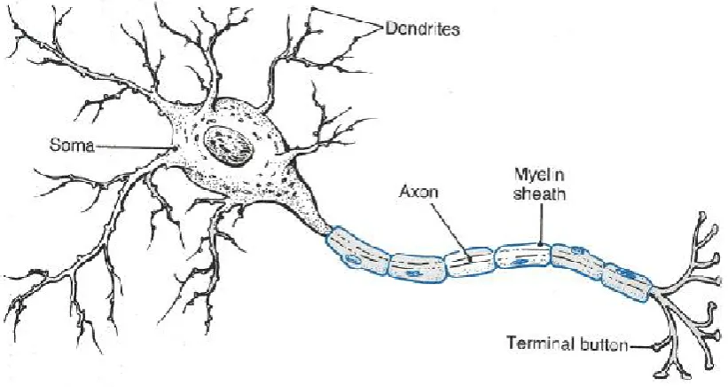
2.1.1 Neurons

At the lowest level, the brain (like the entire nervous system) consists of nerve cells, or neurons. Neurons are cells specialized for the transmission and processing of signals through a variety of electrochemical mechanisms.

They are heavily branched; this structure is called the dendritic tree. The end of the axon (the axon terminal) is where the connection between neurons is made; this is called a synapse.

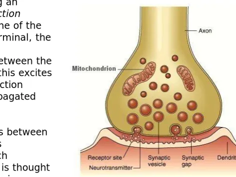
Neurons communicate by passing an electrical impulse known as anaction potentialacross the cell membrane of the axon. Upon reaching the axon terminal, the axon releases chemicals called

neurotransmittersinto the gap between the axon terminal and the dendrite; this excites the dendrite into generating an action potential of its own, which is propagated toward the soma.

The formation of new connections between neurons, coupled with continuous

adaptation of the influence of each

connection (the synaptic weight) is thought to be the method by which the brain

continues to learn throughout life.

Given the diversity of functions performed by the nervous system, it is no surprise that neurons come in a great variety of forms, distinguished by, among other characteristics, polarity, location, size, effect on other neurons and the specific neurotransmitters used. Of specific interest are the so-calledpyramidal neurons

which comprise about 80% of the neurons in the cerebral cortex. The synchronized post-synaptic (i.e. in the dendrites) action potentials of these cells are what

generates thelocal field potential, which is the electrical field that is measured by both EEG and ECoG, as well as implants.

2.1.2 Organization

Anatomically, the central nervous system consists of the brain and the spinal cord. The brain itself can be divided into three parts, the hindbrain, midbrain, and forebrain. The hindbrain and midbrain are the older, more primitive parts of the brain, and are chiefly responsible for autonomic functions. Of more interest is the forebrain or cerebrum, in particular the cerebral cortex.

The cortex (Latin for ‘bark’ so named for its folded and wrinkled appearance) forms the outside of the cerebrum. In humans, the cortex consists of six layers of nervous tissue (distinguished by type of neuron) and is extensively folded, greatly increasing the surface area while keeping the volume manageable. The fissures are called sulci

(Latin for ‘furrow’, singularsulcus) while the ridges are known asgyri(singular

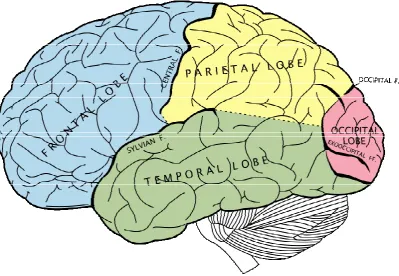
gyrus). Theneocortexis the most recently evolved part of the cerebral cortex. In humans, the neocortex covers approximately 80% of the cerebral cortex. It is

divided into thefrontal,parietal,temporal, andoccipital lobes. All four lobes are split in two by thelongitudinal fissure, diving the cerebral cortex into the two

hemispheres. Oddly, the hemispheres correspond to the opposite side of the body; the left hemisphere controls the right side of the body and vice versa.

Trying to determine precisely where in the brain certain functions are located is extremely difficult, and is likely to remain an active area of research for quite some time. The brain’s information processing capabilities are based on massive

parallelism; no particular area operates entirely alone. Any function performed by a given area could very well be influenced by another in a variety of ways, and have the same effect elsewhere in turn.

Even so, general locations for many brain functions have been determined, often by studying the effects of brain damage to a person’s behaviour and capabilities. It is important to remember, however, that these attributions are oversimplifications.

The frontal lobe is the area of the brain where conscious thought, reasoning, and personality are located. It is located at the front and top of the cerebrum, delineated from the parietal and temporal lobes by thecentral sulcusand the lateralorSylvian sulcus, respectively.

Of particular interest is theprimary motor cortex. Located just anterior of the central sulcus (as well as extending partway into the sulcus), it is directly responsible for executing movement. Axons from this area reach down into the brainstem and the spinal cord, where they connect to lower motor neurons, which pass stimuli on to the muscles.

Interestingly, the primary motor cortex constitutes a map of sorts of the entire body. Areas of the cortex that control adjacent parts of the body are located next to one another. The control area for the legs are located at the top of the brain, the head and face at the other end, near the lateral sulcus. The most surface area is taken up by the arms and hands.

This arrangement has been called the motor homunculus (‘little man’). It is the basis of many BCI systems; since movement (or imagined movement) will predictably

activate certain areas of the primary motor cortex, imagined movement can be used to control the system.

The parietal lobe lies on the top of the cerebral cortex, wedged in between the central, lateral, and parieto-occipital sulci. It is involved in integrating somatosensory information. The

primary somatosensory cortex is located on the posterior side of the central sulcus, adjacent to the primary motor cortex. It has the same type of somatic mapping. Other functions of

the parietal lobe include the integration of visual and spatial information.

The temporal lobe is where theprimary auditory cortexis located. It is also involved in memory, and different forms of semantics.

Finally, the occipital lobe is devoted mostly to visual processing. Visual information is fed into theprimary visual cortexfrom the optic nerve via the thalamus. The

information is then passed on from the primary visual cortex towards both the parietal and temporal lobes. The path to parietal lobe (the dorsal stream) is concerned with spatial relations and integrating the visual information with

somatosensory information. Theventral stream passes into the temporal lobe. It’s function is recognition of objects and the formation and retrieval of memories.

2.1.3 Neuroplasticity

Neuroplasticity refers to the phenomenon where the brain alters its own

organization. Previously, it was thought that many parts of the brain become fixed after formation. One example is the acquisition of language; if a child is not exposed to language during the first few years of life, it becomes very difficult to learn to speak at a later age.

Studies done during the last several decades however, have shown that the brain is a great deal more flexible. It is capable of “re-wiring” itself on almost any level of organization in response to experience or, sometimes, trauma.

Neuroplasticity is a key concept in brain-computer interfaces. When presented with feedback, the brain will adapt. The result is that artificial additions to the usual output paths of the brain, such as controlling a cursor on a computer screen, are incorporated into the functionality of the brain itself. It is hoped that this ability to rewire itself will lead to, among other things, artificial limbs that feel, to the user, like a part of themselves.

2.2 Neuroimaging

Neuroimaging refers to the body of techniques used to derive an image of the brain. It can be divided into two types: structural and functional neuroimaging. The first is concerned with determining the physical structure of the brain; it is used to reveal, for example, tumors or brain injury. Functional neuroimaging is concerned with the activity of (a part of) the brain. It is used to build BCIs, as well as to diagnose neurological conditions such as Alzheimer’s disease or epilepsy. These are not

mutually exclusive, some neuroimaging techniques can be used for both structural and functional neuroimaging.

In this section we will briefly summarize methods of neuroimaging that have been used for BCIs.

2.2.1 Invasive methods

Invasively measuring the activity of the brain amounts to nothing more than opening up the skull and placing electrodes in the appropriate location. Two types can be distinguished: implants that actually penetrate into the grey matter, and those that do not.

2.2.1.1 Intracortical implants

These are electrodes that have been implanted directly into the cerebral matter itself, either directly connected to one or more neurons, or simply sensing the local field potential.

For obvious reasons, most research in this area has been done on animals, often Rhesus monkeys. In one study, monkeys were able to operate a robotic arm remotely. In humans, the focus is on restoring vision to blind people, and neurally-controlled prosthetics, with clinical trials in the preliminary stages. Also, brain pacemakers have been used to artificially stimulate specific areas of the brain to relieve the symptoms of afflictions like Parkinson’s and depression.

Intracortical electrodes provide the highest resolution of any method, with the ability to measure the activity of a single neuron or small samples of neuron (on the order of tens of neurons). However, because of the severity of the surgery involved, they will most likely not be used for BCI systems intended for use by healthy people in the near future.

2.2.1.2 Electrocorticography (ECoG)

Electrocorticography records brain activity using a number of electrodes (usually a grid or strips) that are applied underneath the skull and the dura mater (the outer and toughest of the three membranes making up the meninges) but outside the brain itself. Since the electrodes are effectively lying on top of the cerebral cortex, ECoG has a much higher spatial resolution than EEG, where the presence of the skull mixes and attenuates the signals. Because of this, it can also record higher

frequencies that are blocked entirely by the skull.

ECoG is used clinically as a diagnostic tool for sufferers of intractable epilepsy. ECoG is used to precisely map out the epileptogenic zone prior to resectioning surgery. For BCI systems, ECoG represents a compromise between intracortical implants and non-invasive methods. Because it does not break the blood-brain barrier, the risks of rejection are reduced, while it delivers data of a higher quality than most non-invasive methods.

2.2.2 Non-invasive methods

2.2.2.1 Electroencephalography (EEG)

EEG is the oldest technique for recording brain activity, going back to the first half of the 20th_{century. It is widely used for both clinical and research purposes, and is by}

far the most commonly used method for BCI.

EEG records the local field potential using a number (ranging from tens to 256) of electrodes that are in contact with the scalp, usually with the aid of conductive gel. Every electrode is then connected to an amplifier, which amplifies the signal (which is in the range of tens of microvolts) 1,000 to 100,000 times.

EEG suffers from several limitations. The spatial resolution is very limited; the field potential recorded consists of the net result of the activity of many thousands of neurons. Additionally, the parts of the cerebral cortex that are located inside the sulci, which are located further away from the scalp, contribute much less to the recorded signal. Making things even worse, the signal has to penetrate the meninges and the skull, mixing the signal and making it impossible to precisely determine the source of a specific signal.

EEG is also sensitive to interference from several sources. Externally, electrical devices such as mobile phones can interfere with the recordings. (Most EEG amplifiers are in fact designed to filter out the nigh-ubiquitous 50 and 60 Hz interference from power lines.) Internally, muscle activity and eye potentials (the potential difference between the front and back of the eyeball), both of which are several orders of magnitude greater than brain signals, can cause significant problems.

On the other hand, the temporal resolution of EEG is quite good; up to 1000 Hz. Despite EEGs limitations, its ease of use and relatively low cost make it the most commonly used form of neuroimaging.

2.2.2.2 Magnetoencephalography (MEG)

The same synchronized electrical activity that gives rise to the local field potential measured by EEG, as any electrical current, also

generates a magnetic field that is orthogonal to that current. These magnetic fields can be detected using extremely sensitive

magnetometers known assuperconducting quantum interference devices (SQUIDs)to map the electrical activity. As these magnetic fields are extremely weak (on the order of femtoteslas, or 10-15 _{T), this requires the}

subject be located inside a room specially sealed against magnetic interference.

MEG has a better spatial resolution than EEG, since magnetic fields are less affected by the skull then electrical fields. On the other hand, they also decay faster with distance, making MEG more sensitive to superficial activity. While MEG has been used in BCI in a research setting3_{, the high cost of the device is likely to}

preclude its use in practical applications. One possible application is the use of MEG to obtain detailed data that can then be used to train a EEG-based BCI system.

2.2.2.3 Functional Magnetic Resonance Imaging (fMRI)

Magnetic Resonance Imaging was developed as a medical imaging technology. The subject undergoing scanning is placed inside a powerful magnetic field, aligning the atomic nuclei with the magnetic field lines. Under these conditions, these nuclei will absorb certain frequencies of radio waves. This is known asnuclear magnetic resonance. Different nuclei will absorb different frequencies, for a given field

strength. By pulsing a second magnetic field at the resonance frequency for a chosen type of nucleus (usually protons, or hydrogen nuclei, as these are abundant in living tissue in water molecules) some of these nuclei can be pushed out of alignment. When drifting back into alignment, the protons emit detectable radio frequencies. Depending on the molecule the hydrogen atom is part of, these frequencies will be slightly different, allowing an image of the makeup of the tissue to be constructed.

While MRI can provide a highly detailed image of the structure of tissues, it does not show the metabolic activity, e.g. brain activity. Functional MRI is a form of MRI that measures brain activity by using MRI to measure the blood oxygenation in the brain. When neurons are active they consume a great deal of oxygen; as such, the oxygen level of the blood is a good indicator of activity. Oxygen is carried in the blood bound to hemoglobin molecules; the magnetic resonance frequency of hemoglobin is slightly different depending on whether it has oxygen molecules bound to it. In this way, local brain activity can be measured.

fMRI has spatial resolution on the order of millimeters. Temporal resolution is much lower, on the order of several seconds, since the hemodynamic response is slower than the neural activity it reflects.

fMRI has been used for BCI in the laboratory. In a study by Weiskopf et. al4_subjects

could learn to control their hemodynamic response in the supplementary motor area and parahippocampal place area. More recently, researchers at the University of California succeeded in identifying the pictures that a subject was looking at by analyzing the brain activity using fMRI5_.

2.2.2.4 Electromyography (EMG)

Not a neuroimaging method as such, but since it has been used for/as a component of BCI systems it is mentioned here for completeness. EMG uses the same electrodes as EEG, but instead of recording electrical signals given off by the brain, it records the electrical activity associated with muscle contraction and relaxation.

While this is not strictly BCI, as the interface is not established with the central, but rather the peripheral nervous system, it can be used in much the same way, for example to give paralyzed people control of a mouse cursor (as long as at least some muscle control remains).

2.3 Physiological phenomena used by BCIs

Currently existing BCI systems can be categorized based on the specific signals they utilize. In this section, we will describe these phenomena, followed by a brief

description of BCIs using them.

2.3.1 Brain waves

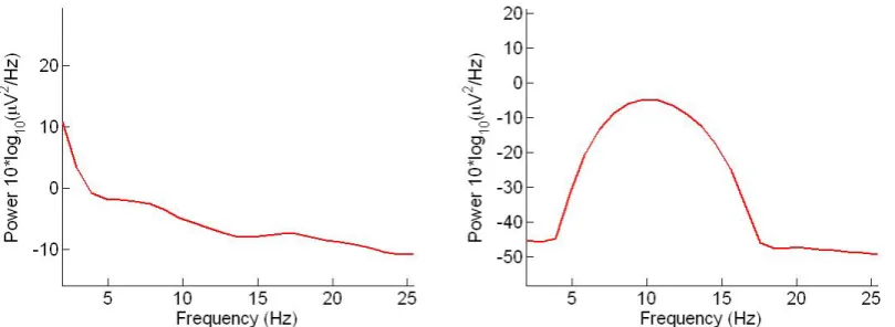
• Alpha: high amplitude signals over the occipital lobes in a range of 8-12 Hz. Alpha waves are thought to be the visual cortex’s idle rhythm; they decrease in amplitude when processing visual information.

• Beta waves range from 12 to 30 Hz. They are associated with concentration and high mental activity.

• Gamma waves: sometimes considered part of the high end of the beta range, from 24 to up to as much as 100 Hz.

• Delta waves are very low frequency, up to 3 Hz. Associated with slow-wave sleep states.

• Theta waves are 4-8 Hz and are also associated with some sleep states as well as with memory.

• Mu waves occur in the same frequency range as alpha waves, but over the motor areas rather than the visual cortex.

Mu waves in particular can be used for BCIs. When moving, the mu rhythm over the corresponding area of the contralateral motor area is decreased. After movement, the mu rhythm increases. This so-called event-related (de)synchronization

(ERD/ERS) occurs even if no movement is actually made; simply imagining motion has the same result. It is possible to distinguish between several types of imagined movements (e.g. either the hands or legs), in order to drive a BCI.

Another way to use brain rhythms is the Brainball game6_{. In this game, the ratio}

between alpha and beta strength is used as a measure of relaxation. Of two players, the one with the most relaxed state will cause a ball lying on a table to move toward the other players, eventually scoring a goal.

2.3.2 Evoked potentials

Evoked potentials are changes in voltage that occur as the result of some sort of external stimulus. Both stimulus and response can be anything in principle. In BCIs, two types are generally used: visual evoked potentials and P300.

2.3.2.1 Visual evoked potentials (VEP)

VEP-based systems generally attempt to use the recorded brain activity to determine which of several presented visual stimuli the user is looking at.

Lalor et al7 _{used steady-state VEP as a means to control a 3D game called}

MindBalance. Steady-state VEP refers to the different visual stimuli being

distinguished from one another by frequency. In the game, the character walks along a tightrope, holding a pole with a black and white checkered flag at each end. At times, the character falters and starts to list to one side; the player must correct for this by looking at the opposite flag. The two flags flicker; one at 17Hz, the other at 20 Hz. The game determines which flag the player is looking at by extracting this frequency from the activity of the visual cortex.

BCIs of this type extract information primarily from EEG recorded from the back of the head, where the visual cortex is located. Because of this, interference from blinks and eye movements is reduced. One downside is that operation requires the subject to be able to direct their gaze, and as such is problematic for those who are

completely paralyzed.

2.3.2.2 P300

has been called the brains “a-ha” response. It is, in effect, the brain sitting up and taking notice.

An advantage of BCIs based on the P300 response is that no training is required; it is an innate response. At the same time, it is unclear how the P300 response changes in the long term when used as a basis for BCI.

The P300 response has been employed in a number of BCIs, notably by Donchin et al8_{. The user faces a 6x6 matrix of letter and digits. Every 1/8 s, one row or column}

is highlighted. The strength of the P300 response is computed for every time a row or column flashes. This strength is significant only for the row and column containing the desired choice, thus revealing which character the user intended.

2.3.3 Slow cortical potentials (SCP)

Caused by synchronous depolarization of the apical dendrites in the upper layers of the cortex, slow cortical potentials have some of the lowest frequencies of all EEG features. They manifest as a positive or negative shift in potential and can last from 0.5 second up to 10 seconds. SCPs are considered to reflect a self-regulatory mechanism of the brain; positive shifts are seen during periods of activity and lead to an increase in the inhibition of neuronal activity, preventing overexcitation. Similarly, negative shifts represent increased excitability and a state of readiness. In studies over more than 30 years, Birbaumer et al demonstrated that using visual, auditory or tactile feedback, people can learn to regulate SCPs. This forms the basis of a BCI known as the TTD (thought translation device) which has been used to restore basic communication capability to people with late-stage ALS.9

2.3.4 Cortical neurons

This last form of BCI uses intracortical microelectrodes to directly record action potentials from cortical neurons. This form of BCI is actually one of the oldest; in experiments done during the late 1970s several studies showed that using operant conditioning, monkeys could learn to control the firing rate of recorded neurons.10,11

It was not until the 1990s that electrodes suitable for human use became available. In one case12_{an almost completely paralyzed patient used an implanted electrode to}

spell at a rate of about 3 letters per minute. The first commercial brain implant, BrainGate, developed by the bio-tech company Cyberkinetics in conjunction with the Department of Neuroscience at Brown University is currently undergoing clinical trials.13

3 Computational methods in BCI

Following signal acquisition, the actual task of translating the recorded signals into commands begins. The process of mapping brain signals to a small number of classes (each representing a possible command) is generally divided into several subtasks. Pre-processing is concerned with preparing the data, removing noise and

artifacts, and otherwise improving the quality of the data. Feature extraction distills the pre-processed trials, which can be quite large, down to a small number of features. The feature extraction process is usually designed with the specific characteristics of the targeted phenomenon(s) in mind. Others, like autoregressive models, may not be directly linked to a specific phenomenon, while still showing discriminating capability. Optionally, post-processing can be applied to reduce the size of the feature vector. And finally, a classifier determines the class of the trial.

In this chapter we will discuss some algorithms and mathematical models commonly used in BCI systems.

3.1 Preprocessing steps

3.1.1 Time-frequency analysis

Feature extraction methods generally attempt to isolate one particular

neurophysiological phenomenon, which is usually found only in a specific frequency range. The purpose of time-frequency analysis is to filter out signals outside a

certain frequency range. The chosen range depends on the type of brain wave that is expected and the amount of variability in which frequency this wave is usually seen. For example, mu waves occur mostly over the range of 8-13 Hz, however larger ranges have been used.

Pre-processing Feature

Extraction Post-Processing Classification

Signal Acquisition

Class labels

3.1.2 Down sampling

Frequently, BCI systems use EEG equipment which delivers the recorded brain signals at a sampling rate far higher than needed. Since the highest frequency brain waves of interest are no higher than 40-50 Hz at most, down sampling the signal is a common method used. As long as the sampling rate is not reduced too much, it should not adversely affect the classification performance while greatly reducing memory and processor load.

3.1.3 Independent Component Analysis

ICA separates the measured signals into maximally independent source signals. This is potentially very useful in processing EEGs, since the recorded signals are mixed and attenuated by the skull. For ECoGs, where the recording electrodes are in direct contact with the brain, ICA is not expected to be very helpful.

ICA assumes independent, non-Gaussian sources that linearly combine at the sensors with no time delay:

x = As, s = A-1_x

where sis the source vector andxthe sensors. LetW be an estimator ofA-1_{, andy}

and estimator of s. wiis a row of W, andyi= wiTx.Wis calculated by exploiting the

central limit theorem, which states that the sum of independent random variables tends towards a Gaussian distribution as the number of variables increases.

Therefore, because the components ofxare a weighted sum of the (non-Gaussian) components of s, xis more Gaussian than s.W can now be found by finding thosewi

that maximize the nongaussianity ofyi. For this, some measure of nongaussianity

must be chosen. Common choices are kurtosis or an estimation of negentropy.

3.2 Feature Extraction

3.2.1 Common Spatial Patterns (CSP)

Common Spatial Patterns, described by Koles et al.14_{, applies a linear transformation}

to the data, projecting the original channels onto an equal number of surrogate channels in a way that maximizes the between-class difference in mean variance. Since channel variance in band-pass filtered data is a measure of signal strength, this can be used to detect event-related desynchronization resulting from motor imagery.

The following paragraphs will describe the basic CSP algorithm, as well as a number of modifications that exist.

3.2.1.1 Basic CSP

The method of CSP takes the measurements of a trial of classain the form of an N channels by T samples matrix Vi

a. The columns of all matrices (trials) are then

interpreted as a point cloud in N dimensions. The trials have previously undergone band-pass filtering, so the mean of the distribution is zero. Ri

ais the covariance

14_{matrix normalized with the total variance of triali, andR}

ais the average covariance

withRi

bandRbequivalent for classb. The composite covariance matrixRc=Ra+Rb is

subsequently factored into it’s eigenvectors as follows: T c c

c

B

B

R

=

Λ

Bcis the N x N matrix of normalized eigenvectors, and ?Ythe matrix of the

corresponding eigenvalues. The whitening transformation T

c

B

W

=

Λ

equalizes the variances of the space spanned by the eigenvectors, so that WRcWT=I.

The whitening transformation scales the point cloud to have a variance of one in all dimensions, effectively turning it into white noise. Individually transformingRaand Rbin this way

results in matrices SaandSbwith identical eigenvectors and complimentary

eigenvalues:

The difference between the classes is greatest along those vectors in Uwhere the corresponding eigenvalues differ the most. Therefore, when the trials are the whitened and projected ontoU

i

those directions are maximally suited to distinguish between the two classes. In other words, when sorted in order of ascending eigenvalues for one classa, the first row of the transformed matrix has maximum variance for the trials of class a

and minimum variance for class b, and the last row has minimum variance for the trials of class aand maximum variance for classb. The variances of the first and last

m rows are used as features, after being normalized by the sum of the retained variances and log-transformed:

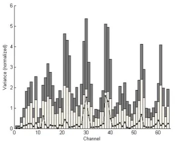
Figures 1 and 2 illustrate the way CSP operates. The stacked bars represent the variance per channel (normalized to have a mean of one, for purposes of

Most of the CSP algorithm does not strictly qualify as feature extraction; rather it is a form of preprocessing. The only part that actually extracts any features is the

calculation of the normalized log-variance. Because CSP is specifically designed to maximize separability in channel variance, it is usually considered as a whole.

As the name implies, CSP does not take the time factor into account; merely location. Since we expect certain movements to activate certain areas of the brain, this is useful. However, that activation will occur only in a limited frequency band, prompting the use of temporal filters such as band-pass filters.

A so-far unresolved weakness of CSP is it’s tendency to overfit. The reliance on equalizing the variance means that small shifts in variance distribution (which, given the random nature of EEG signals, are commonplace) can cause a significant

increase in classification error.

3.2.1.2 Multi-class CSP

A shortcoming of CSP is that it was designed for discriminating between only two classes of input. This limits the bandwidth of CSP-based BCI systems to 1 bit per trial. Several extensions have been proposed to extend CSP for the multi-class case. One approach, used in15_{, is to simply leave the algorithm as-is, compute pairwise}

classifications and use a voting scheme to determine the final classification.

Another is to use a One-Versus-the-Rest (OVR) approach15,16_{. As the name implies,}

OVR extracts spatial patterns common to one class by regarding all other classes as one class, repeated for all classes. So, instead of calculatingSaandSbas in the basic

CSP algorithm, we calculate:

T a a

T a

a

WR

W

S

WR

W

S

=

,

=

where

R

=

∑

R

,

x

≠

a

Both these methods still use the same binary algorithm; specifically, the

simultaneous diagonalization of the mean covariance matrices of the two classes. The goal of this operation is, given the mean covariance matrices oficlasses

R

S

=

WR

W

∑

S

=

I

diagonalization (JAD). Another difficulty with this method is that, unlike the binary

Figure 10 - Mean variance per channel per class on the pre-CSP training set (stacked bars).

case where one simply sorts Wby eigenvalue, it is not obvious which spatial patterns are optimal with respect to discriminating between classes. Grosse-Wentrup and Buss17_{and the references therein provide more information on JAD and the problem}

of selecting optimal spatial patterns.

3.2.1.3 Spectral CSP

The use of a band-pass filter prior to CSP, while necessary, can also be a weakness. It is desirable to filter out as much frequencies as possible, leaving only those with the highest information content. Unfortunately, the distribution of discriminative information content varies from person to person. Whereas one subject might

achieve optimal performance with a 12 Hz filter, another might be better served with 8 Hz. Spectral CSP attempts to improve discrimination by optimizing, in addition to the spatial filters, a spectral filter as well.

Common Spatio-Spectral Patterns (CSSP)18 _{works by concatenating the signals}

iwith

i

s

projection vector Wwhich is composed of Nspatial filters andNspectral filters, defining a finite impulse response filter (FIR) for each channel.

Lemm et al found that improvement of CSSP over CSP is heavily dependant on the choice of tÉ, although almost any choice of tÉconstituted an improvement. The optimal choice for t was chosen by cross-validation on the training set. CSSP is not necessarily limited to one block of delayed channels, but it was found that, in most realistic cases, one delay tap was most effective.

Proposed in [19_{], Common Sparse Spectral Spatial Patterns attempts to learn a}

complete spatio-temporal filter. A FIR filter can be defined by a sequence b so that

y(t)=b1x(t)+b2x(t-1)+…+bnbx(t-nb-1). A fixed lengthnbis chosen andb(1)=1. Given

For anyb, we can use CSP to calculate the optimalW, leaving anb-1-dimensional

optimization problem. To restrict the complexity of the solution and prevent

overfitting, a regularization constant is used, which restricts the solutions to sparse ones, i.e. solutions forbthat only have a few non-zero entries. This constant has to be chosen through cross-validation.

3.2.1.4 Common Spatial Subspace Decomposition

CSSD20_{places some additional interpretation on the signal matricesX}

aandXb. It

uses a spatio-temporal source model modelingXaandXbas follows:

[

]

[

]



where SaandSbare sources specific to classaandb, Scare sources common to both

classes, andCa, CbandCcare the corresponding spatial patterns. Using spatial

subspace analysis, the subspace spanned by the common patternsCc is eliminated,

leaving the patterns particular to the classes.

3.3 Post processing

However, when feature vectors are of a high dimensionality, such as when several feature extraction methods are used in parallel, it can be occasionally useful. Just about any of the standard dimensionality reduction techniques can be used, a common choice is Principal Components Analysis.

3.4 Classification

For classification any of the standard machine learning techniques can be used; there does not appear to be much advantage in using one particular type of classifier. The primary reason for this is simply that the feature extraction methods are designed to maximize separability; it has already done most of the work, so no advanced

classification techniques are needed. Common choices are support vector machines (SVM), neural networks, Mahalanobis distance, linear discriminant analysis (LDA) or some combination thereof.

4 Analyzing generalization over time

The first step in improving generalization over time properties of BCI methods is to determine how the nonstationarity inherent to brain waves manifests in the feature vectors that are derived from them. In this chapter we will examine the influence of nonstationarity on a basic CSP-based classifier.

4.1 Methodology

The purpose of this research is to evaluate methods used for BCI on their

generalization over time, and to investigate how this can be improved. To this end, using the dataset described above, we will start with an experiment in a simple setup that will serve as the baseline to further inquiries.

4.1.1 Dataset

The data used in this research was obtained from the BCI Competition III21_{. The}

dataset was provided by the University of Tübingen and recorded by Lal et al22_.

The subjects involved in the recording were patients suffering from focal epilepsy, in which the source of the seizures is only a portion of the brain. In order to precisely localize this epileptic focus the patients had electrodes implanted underneath the dura mater, on the surface of the brain itself. These electrodes were connected to a

recorder for a period of 5-14 days. These recordings allow doctors to localize the focus prior to surgery.

The dataset consists of data recorded from one subject, who had been

implanted with a platinum electrode grid consisting of 8x8 electrodes,

approximately 8x8 cm in size. The grid was placed on the right hemisphere of the brain, covering the primary motor cortex and premotor areas as well as adjacent areas unrelated to motor control such as the primary somatosensory cortex.

The subject was asked to imagine either moving the left little finger or the tongue, as indicated by a visual cue, for four seconds. The trials in the dataset consist of 3 seconds of recordings, starting 0.5 seconds after the visual cue had ended in order to prevent visually evoked potentials from affecting the data.

The dataset consists of a training set of 278 trials, and a test set of 100 trials, recorded approximately one week after the training set. Each trial consists of 3 seconds of brain activity, recorded at 1000 Hz from 64 channels.

In the experiments described in this chapter we will randomly split the training set into two parts. The first part is what we will use to train the classifiers, and so when we refer to thetraining setfrom now on, we will be referring to this subset, and not the original 278-trial training set. The remainder we will refer to as thevalidation set; this set will be used to measure the classification error of the classifier. This

error rate will then be compared to the error rate incurred by thetest set, which is the 100-trial set that was recorded later.

The purpose of this is to get a measure of the performance degradation that occurs through variation in the signal over time. Note that this disregards any variation within the sets; it treats that as part of the ‘normal’ variance of the signal.

4.1.2 Characteristics

The use of data obtained by ECoG rather than EEG has a number of ramifications for the applicability of this research to practical BCI applications, most of which can be expected to not involve major surgery, at least for the immediate future.

The first major difference is the higher spatial resolution of ECoG. A single electrode records the potentials of a much smaller part of the cerebral cortex when compared to EEG, where the presence of the skull and several layers of tissue mixes and

attenuates the signals. For the same reason, ECoG recordings suffer to a much lesser extent from the artifacts caused by muscle movements and eye potentials that plague EEG.

This generally higher quality does not directly affect the primary focus of this research, i.e. the generalization over time properties of the methods under

investigation. However, the fact that ECoG uses implanted electrodes does eliminate one of the sources of poor performance during subsequent sessions in EEG-based BCI systems. In such systems, the electrodes have to be re-applied for every session. As a result, electrodes may be placed in a slightly different location, or the conductivity of the contact between electrode and scalp may be different, either from varying amounts of conductive gel or from natural variations in skin conductivity over time.

The degree to which these factors contribute to reduced performance on later sessions is unknown, and may be a venue for future research.

4.2 Baseline experiment

The baseline experiment will be used to quantify any degradation in performance that occurs over time and to attempt to find the underlying cause(s). We will use a CSP-based system using multiple classifiers. The reason for this that CSP is a commonly used technique for BCI systems, with a great deal of available literature. The use of multiple classifiers is intended to show if there is significant difference in performance; given the literature, this is not expected.

4.2.1 Setup

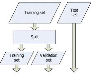
The baseline experiment as well as follow-up experiments will use the same basic framework, as shown in the figure below.

Training set Test

The setup for the initial experiment is fairly basic. The preprocessing consists of a band-pass filter, followed by down sampling of the filtered trials to reduce memory and processing requirements. Feature extraction consists of projecting the trials onto the spatial filters derived by CSP algorithm from the training set, and computing the variance of each projected channel as described in 3.2.1.

Several machine learning techniques will be used to classify the feature vectors, to see if there is a significant difference in their performance. The classifiers used will be a linear classifier based on the Fisher Linear Discriminant, a Support Vector Machine, and two neural networks, one a single perceptron and one a multilayer perceptron with four neurons in the hidden layer.

This setup has three parameters: the frequency band used by the band-pass filter, the new sampling rate, and the number of channels retained from the transformed trials (which determines the dimensionality of the feature vector). Based on the literature, we will use a frequency band of 8-13 Hz, a 100 Hz sampling rate, and retain the variances of the two first and last channels of the projected trials, for a four-dimensional feature vector. The training set will consist of 200 trials, 100 of each class; the remaining 78 trials will make up the validation set.

4.2.2 Results

The following table shows the result of the baseline experiment. Since the training and validation sets are randomly drawn from the original training set, we table shows the means and standard deviation over 30 iterations.

Validation set Test set

FLD 12.69 0.0368 19.60 0.0365

P 15.90 0.0699 21.90 0.0612

MLP 16.50 0.0871 25.40 0.0930

SVM 13.08 0.0387 23.07 0.0569

FLD

34.7667 (1.8323)

47.8 (1.2429) 4.2333 (1.8323)2.2 (1.2429)

5.6667 (2.3243)

17.4 (3.5096) 33.3333 (2.3243)32.6 (3.5096)

P

32.4 (6.6726)

46.0667 (5.4135) 6.6 (6.6726)3.9333 (5.4135)

5.8 (4.7518)

17.6997 (8.8297) 33.2 (4.7518)32.0333 (8.8297)

Preprocessing

MLP

32.0667 (4.6904)

45.3 (4.3482) 6.9333 (4.6530)3.9333 (3.8857)

5.9333 (2.8154)

21.4667 (10.8524) 33.0667 (2.8154)28.6667 (10.7366)

SVM

34.6667 (1.9889)

48.2667 (1.2299) 4.3333 (1.9889)1.7333 (1.2299)

5.8667 (2.6747)

21.3333 (6.1775) 33.1333 (2.6747)28.6667 (6.1775)

Table 1 - Results of the baseline experiment. Top: error rates and standard deviation. Bottom: confusion matrices per classifier, standard deviation in parentheses, test set in italics. Numbers are mean recognition counts, not percentages.

As can be seen in the table, there is not a great deal of difference in performance between the different classifiers. The neural network-based classifiers perform slightly worse than the other two. They also have a higher variability in their performance, as seen in the higher standard deviation.

While interesting, these differences are not statistically significant. Comparing the error rates using one-way analysis of variance (ANOVA) and the Kruskal-Wallis test yields a 26.08% and a 39.85% chance respectively of all tests having the same mean error rate.

It should be noted that the data violates some of the assumptions underlying these tests; specifically the assumption of the sample points being normally distributed (ANOVA) and of equal variance (both ANOVA and Kruskal-Wallis). However, since violation of these assumptions results in a greater chance of the null hypothesis being rejected, which is not the case here, we can safely assume that the conclusion in this case is correct.

With regards to generalization over time, all classifiers show the same behaviour on the validation set: the error rate increases approximately 5-10% and the standard deviation increases slightly. The Fisher Linear Discriminant again performs the best; it not only has the highest recognition rate (although not by much), but is also the most reliable, with a standard deviation 1.5-2.5 times smaller.

4.3 Analysis of baseline experiment

First, let us look at the outputs of the CSP algorithm itself. In the following plots every bar represents one channel. The bottom bar represents the mean value of the normalized and log-transformed variance of the channel for class 1, the top bar for class 2. The dots are the difference between means of the two classes.

Figure 15 - Mean normalized log-variance per channel after CSP on the training set, stacked bars indicating class. Dots signify between-class difference.

As expected, on the training set the mean variances for both classes add up to approximately the same across channels, with the difference between classes greatest in the first and last few channels.

On the validation set, although it is drawn from the same distribution, it can be seen that the difference between classes is shrinking; while the outer channels still have a large distinction between classes, it drops off faster, and the middle channels in particular fluctuate apparently randomly between the training set value and almost zero.

When we look at the test set, two things stand out. First, the differences between classes look mostly the same compared to the test set. Most middle channels still fluctuate in much the same way, while the first few are still approximately the same. Secondly, the mean variance is no longer the same across channels. What this means for the derived features can be seen in Figure 17:

These are the actual values used by the classifiers, i.e. the variances of the first and last projected channels, normalized to add up to one, log-transformed and plotted in 2D. Channels 2 and 63, omitted from the plot, show a similar pattern.

It is clear that in all cases there is a certain amount of overlap between classes, so perfect classification is not possible in any case, but this is hardly surprising. When comparing the sets, the validation set looks very much like what is: additional samples drawn from the same distribution. The test set also looks roughly similar; the samples are a little more spread out, but their relative position is mostly the same. In relation to the training and validation sets, however, the test set as a whole has moved. In other words, the difference between classes is similar, but the mean has shifted.

4.4 Conclusions

As described in paragraph 3.2.1, the CSP algorithm uses channel variance as a measure of signal strength, maximizing the between-class difference in variance on the training data. The main source of nonstationarity when classifying this dataset using CSP is a shift in the distribution of strength between the signals recorded from the portions of the brain relevant to the task and those that are not. As a result, the feature vectors derived from the test set are shifted compared to those derived from the training set.

This shift is most likely inherent to CSP-based BCI systems; since the whitening transformation equalizes the mean variance of all channels, any change in relative signal strength between the channels will be reflected in the variances of the surrogate channels. Even if the signal strength in the area of the brain that is activated by the motor imagery does not change at all, any change in another, possibly completely unrelated part of the brain will influence all surrogate channels.

Moreover, the effect of the shift on classifier performance is unpredictable. In the case of the baseline experiment, the shift occurred mostly along the hyperplane separating the two classes, leading to a relatively minor increase in classifier error. There is no guarantee that this will always be the case; the shift could easily deposit the entire test set on one side of the hyperplane, causing an error rate of 50%.

5 Improving generalization over time

Having seen in chapter 4 the effects of nonstationarity on CSP-based classifiers, we will now examine a number of possible ways to correct for the observed shift of the feature vectors, evaluating them for improvements in performance.

5.1 Rebiasing

The baseline experiment shows that there is significant performance loss on the test set; clearly some sort of adaptation is needed. As seen, the features derived from the trials using CSP will shift to a new mean over time; however, the distinction between classes remains roughly similar. The simplest way to adjust the classifiers would be to simply shift the feature vectors back to the old mean; this is equivalent to changing the threshold/bias on the classifiers, but is more easily accomplished by subtracting the average vector from the feature vectors.

trials

f

f

f

=

−

In other words, the feature vectors of each set are shifted so that they are centered on the origin. This is done for all three sets separately, reducing the difference between sets, hopefully improving the performance of classifiers trained on one set in classifying the other sets.

Obviously, in the case of the test set this is hardly realistic; the test set represents the BCI system being used after having gone through a training session some amount of time earlier, and during online use the trials would be recorded one at a time, ensuring that the new mean is not yet known. The purpose of this experiment is simply to determine if this approach is viable.

5.1.1 Results

This results in the following performance ratios, again over 30 iterations with a training set of 200 trials.

Validation set Test set

FLD 13.12 0.0379 13.93 0.0216

P 15.21 0.0614 16.93 0.0537

MLP 13.68 0.0320 18.20 0.0497

SVM 13.38 0.0254 13.67 0.0243

FLD

34.1333 (1.6761)

43.5667 (1.6543) 4.8667 (1.6761)6.4333 (1.6543)

5.3667 (1.8659)

7.5000 (1.4563) 33.6333 (1.8659)42.5000 (1.4563)

P

32.7667 (5.2502)

40.8333 (6.3086) 6.2333 (5.2502)9.1667 (6.3086)

5.6333 (4.9024)

MLP

33.3000 (2.5072)

40.2000 (4.8877) 5.4333 (2.2234)9.6667 (4.6781)

5.2333 (2.3295)

8.5333 (3.9977) 33.7667 (2.3295)41.1000 (4.0798)

SVM

34.0667 (1.8925)

43.8667 (1.8144) 4.9333 (1.8925)6.1333 (1.8144)

5.5000 (1.9957)

21.3333 (1.9605) 33.5000 (1.9957)42.4667 (1.9605)

Table 2 - Results of centering. Top: error rates and standard deviation. Bottom: confusion matrices per classifier, standard deviation in parentheses, test set in italics. Numbers are mean recognition counts, not percentages.

It is clear that centering the sets has had its desired effect; while performance on the validation set has remained virtually identical to the baseline experiment, the classifiers now perform almost as good on the test set as well. The loss of

performance is less than 1% for the FLD and SVM classifiers, about 1.5% for P, and under 5% for MLP (which is still significantly less than the 9% drop on the baseline).

5.2 Adaptation - mean

As noted, the centering approach, while effective, it is not very realistic. In the case of a real BCI system, the system would not know how much the features had shifted. In order to be practical, the system would have to estimate the new mean from the trials as they are recorded one by one.

In order to simulate such a system in operation, we will again center the training and validation sets around their mean, but from the trials of the test set we will subtract only the mean of the trials seen so far, i.e.:

∑

This simulates the situation of a BCI system attempting to learn the new mean. We are assuming that the system has no information regarding the class labels of the new trials, which may or may not be the case, depending on the application. (For example, a spelling system can periodically find out whether or not certain classifications were correct, by checking the spelled words for errors.)

In such a system, the new bias being applied to the classifier would at first be very inaccurate, and then converge on the ‘true’ mean. Because of this, the error rate on the whole test set is not of much interest. What we want to know is, how soon does the mean of the trials seen so far approach the true mean closely enough for the classifier to be not much worse than the centered approach above?

To find out, we will randomly shuffle the test set, and then subtract from all trials the mean of the firstntrials. We will refer to this as a window size of n. We then classify the test set, again repeating the procedure 30 times. The assumption is that there are no fundamental changes within the test set, and consequently the order of the trials is immaterial. By centering the entire test set around the mean of the firstn

trials, we can approximate the error rate aftern trials.

5.2.1 Results

It can be seen that the error rate in most cases quickly converges on a value 1-2% above the value on the centered approach, generally within 10-20 trials. Again, the neural network-based classifiers are more unreliable, especially the perceptron.

5.2.2 Discussion

From this experiment, it appears that this simple approach to adaptation could potentially be useful in improving generalization over time in CSP-based BCI systems. There are several possible issues with it however.

Firstly, the experiment assumes there are no fundamental changes within the test set; it only affects generalization from training set to test set. This is out of

necessity; the dataset did not include any information about the order in which the trials were recorded. As such, trying to track changes over the course of the test set, and trying to distinguish those changes from the normal variation is not possible with this dataset.

The most likely approach to deal with such changes would be to use a sliding window to estimate the current mean. From the above result, a window size of approximately 10-20 trials should be adequate. The desirability of a sliding windows algorithm over one used here depends on how likely a fundamental shift like the one between training set and test set is likely to occur during a session. If one does not occur during a session, a sliding window would be slightly less effective than using all trials. On the other hand, if one does occur, it could take a long time before enough trials have been seen to shift the computed mean to the actual mean.

All things considered, for practical applications a sliding window would probably the preferable approach. As can be seen, classification error effectively ceases to drop after 20 trials. Under those condition, the ability to continuously adapt should be considered to be more valuable than a very small increase in performanceifnothing goes wrong.

The second issue in implementing this approach in BCI systems lies in the fact that, as explained in 4.1.2, ECoG suffers far less from artifacts than EEG. Outliers in the feature vectors could well cause the computed mean to shift away from the actual mean.

5.3 Adaptation – mean with minimum window size

In the approach to adaptation used in 5.2, at the beginning of the test set the system starts with a blank slate. The new mean is estimated from the trials of the test set only, ignoring the old data.

For this experiment, we will attempt to use the information from the training set to improve the speed with which the classifier converges by supplementing the padding the feature vectors used to estimate the new mean with training set data. The theory is that on the first few trials, where the inaccuracy is highest, the classifier can benefit from using some information from the training set.



The above formula is identical to the one used in 5.2, except for the introduction of a minimum window sizem. In case the window sizei (i.e. the number of trials seen so far) is smaller than m, the lastm-itrials of the training set are added to the

calculation. When

m

≤

i

5.3.1 Results

The plot is a little crowded, but it is still clear that attempting to co-opt the training set to speed up convergence has had an adverse effect. The higher the minimum window size, the slower it converges. The smallest minimum window size used, 4, is almost identical to the baseline from 5.2. The overall effect is one of increased error rate, which only approaches the base line when the minimum window size

approaches the actual window size, i.e. when the influence of the training data is smallest.

5.4 Adaptation – robustness to skewed test sets

In the tests done so far, we have always randomized the trials before classifying the entire test set (based on the firstntrials). Since the test set consists of 50 trials of each class, this means that the performance figures derived are predicated on a test set with a 1:1 ratio of classes. During online operation of a BCI system, there is no guarantee that this is the case; for a spelling application for example, some letter would be wanted more often than others.

In this paragraph, we will test a number of rebiasing methods that are expected to be less susceptible to skewed input.

5.4.1 Method

In this experiment, we will test a number of methods we hope will have a better performance on a skewed test set. To this end, we construct the test set in such a way that, for every window size, every possible ratio of classes is tested. So, for a window size of 4, ratios of 1:3, 2:2 and 3:1 are tested. Window sizes of two up to

twenty will be tested. As before, each combination of window size and class ratio will be tested a total of 30 iterations.

In the following sections, the methods undergoing evaluation are detailed. In the test, the mean method from 5.2 is also included as a baseline. Only FDA will be used as a classifier, owing to its consistently superior performance and low computational cost.

5.4.1.1 Median

The median, as a measure of the central tendency of a distribution, is generally more robust in the presence of outliers than the arithmetic mean. It is the obvious choice for a rebiasing strategy that can deal better with the effects of a skewed test set.

5.4.1.2 Bounding box

The second method constructs an axis-aligned bounding box around every set, then moves the entire set so the center of the box is on the origin:

{

f

i

n

}

This arrangement is clearly going to be extra sensitive to outliers, as even a single anomalous trial can move the entire set considerably. It is included here more for the purpose of evaluating performance at small window sizes. In the case of, say, a window size of four trials, three of which are of one class, the mean will be skewed toward one side. The bounding box is expected to perform better in these cases; in effect using its sensitivity to outliers as a positive.

5.4.1.3 K-means clustering

As observed in paragraph 4.3, the feature vectors of each set can be seen forming two slightly overlapping but mostly distinct clusters in feature space. Using k-means clustering, we can attempt to separate the test set into these two clusters. This effectively constitutes a form of classification in its own right. Here, we will use it as a means to estimate the mean for rebiasing.

We performed k-means clustering on the trials of the window. Because k-means clustering is a local search method and highly dependant on the initial cluster centroid positions (or “seeds”), we use as initial values the means of the feature vectors for the trials of both classes from the training set, shifted by the difference between means of the overall training set and the window:



Note that this method, unlike the previous methods. uses the class labels of the training set as a preliminary toward estimating the class labels of the test set.

5.4.1.4 Weighted k-means

The k-means clustering method in 5.4.1.3 estimates the means of both clusters by minimizing the sum of squared Euclidian distance from the feature vectors to their respective centroid.

While this will generally give good results, if the vectors from one class in the window are skewed toward one ‘edge’ of the range for that class, k-means will be substantially off from the actual center.

To correct for this, we assume that the difference between classes is constant across sets, i.e. that the distance between the two classes is identical for both training and test set. We then define an error term

c

denoting the probability that a vector xnis the actual center of the cluster n, where cnis the centroid of classn derived through k-means clustering. We then calculate

the x1andx2that minimize the error term, with the added constraint that

1

The midpoint of thesex1andx2is used for rebiasing the test set. The use of

c window

n

(and so a greater degree of certainty) have a greater weight, i.e. the estimated actual centers of the clusters will be closer to a larger cluster.

5.4.2 Results

The effect of skewed data on the baseline method using the mean is as one might expect. As window size increases, average classification error rates drop to around 15% when the class ratio is close to parity. As the class ratio becomes more and more skewed to either class, error rates increase until they approach 25%. This is as expected; when nearly all samples are of one class, this method will rebias the trials around the mean of that class rather than the mean of all classes. For a linear

Figure 20 - Result of the baseline experiment on skewed test windows. The top patch represents the mean error rate, the bottom patch the standard deviation.

Of the four methods under consideration, the bounding box and median are outright failures. Neither drops below 20% error rate even on balanced test windows, and they approach 30% as windows become more skewed.

The median method simply performs in the same manner as the baseline method, only inferior. With the highest window size, it performs about 7% worse than when the test window is balanced, which is around the same as the baseline. Performance is approximately 5% below the baseline across the board.

Figure 21 - Result of the experiment on skewed test windows using the median. The top patch represents the mean error rate, the bottom patch the standard deviation.

K-means performs surprisingly well. Error rates at the very edge of the spectrum of skewness, with only one or two members of one class, are slightly above those of the baseline. When the test window is closer to balanced, performance quickly increases, quickly outperforming the baseline method. In fact, it appears that k-means’ error rate is not so much dependant on the class ratio rather than the number of trials per class; as long as each class has two or three trials, it performs better on average than the baseline.

K-means does have the drawback of being less reliable; the standard deviation of the error rate becomes much higher for skewed sets, unlike the baseline which maintains a mostly stable standard deviation. This is not unexpected; when there are only a few trials of one class, the effect of a misclassification by the k-means algorithm on the centroid position (and thereby the estimated set mean) will be much more severe.

Finally, weighted k-means. While not as bad as median or bounding box-based rebiasing, it performs sub-par with respect to both the baseline and k-means methods. Not only this, but the standard deviation becomes even more pronounced than that of k-means when dealing with highly skewed windows.

For the pu