Dimensionality Reduction
Nicolas BRUNEAU1,2, Jean-Luc DANGER1,3, Sylvain GUILLEY1,3, Annelie HEUSER?1, Yannick TEGLIA2
1 TELECOM-ParisTech,Crypto Group, Paris, FRANCE 2 STMicroelectronics, AST division, Rousset, FRANCE
3Secure-IC S.A.S., Rennes, FRANCE
Abstract. Multi-variate side-channel attacks allow to break higher-order masking protections by combining several leakage samples. But how to optimally extract all the information contained in all possibled-tuples of points? In this article, we intro-duce preprocessing tools that answer this question. We first show that maximizing the higher-order CPA coefficient is equivalent to finding the maximum of the covariance. We apply this equivalence to the problem of trace dimensionality reduction by linear combination of its samples. Then we establish the link between this problem and the Principal Component Analysis. In a second step we present the optimal solution for the problem of maximizing the covariance. We also theoretically and empirically compare these methods. We finally apply them on real measurements, publicly avail-able under the DPA Contest v4, to evaluate how the proposed techniques improve the second-order CPA (2O-CPA).
Keywords:Bi-variate attacks, second-order correlation power analysis (2O-CPA), principal component analysis, interclass variance, covariance vector
1 Introduction
For more than a decade now Side-Channel Attacks (SCA [6]) have been an impor-tant threat against embedded systems. As a consequence protection techniques and countermeasures have been an important research topic. Data masking [9] is one of the most popular protection technique. These schemes have in turn been the target of higher-order SCA [24,18].
In some particular masking implementations, the two shares [16] depending on the same mask leak at different moments (e.g., in software). Second-order attacks that combine two different time samples are calledbi-variate SCA. When the mask-ing scheme uses dshares, multi-variate SCA are still able to reveal the secret key by combining leakage samples corresponding to each of the d shares. Note that, depending on the implementation and the measurement setup each share may leak in multiple samples.
?
To enhance the results of SCA several preprocessing tools can be used. In the case of bi-variate SCA it is particularly interesting to take into account all the information spread over the time. Indeed, the number of possible pairs increases quadratically in the number of leakage samples. For example, if the first share leaks overT1samples and the second share overT2samples, we could perform abi-variate
SCA on T1×T2 possible combined points. So, taking into account all these leaks
may undoubtedly increase the efficiency of an attack.
More generally, to break (d−1)-order masking schemes the attacker needs to combine d samples corresponding to d shares. So, if Ti is the number of samples which leak the i-th share then the attacker could perform multi-variate SCA on
Q
1≤i≤dTi different d-tuples. In other words, the number of possible d-tuples to performmulti-variate SCAis inO(Td) whereT is the number of samples each share leaks (and assuming that each share is leaking the same number of samples, i.e., ∀i∈J1, dK, Ti=T).
Many methods have been presented in the area of SCA to combine the infor-mation spread over time: the Principal Component Analysis (PCA) for dimension-ality reduction [1] for Template attacks [7] but also as a preprocessing tool [2] for DPA [13]. Recently in [11] Hajra and Mukhopadhyay present an approach based on match filters to find the optimal preprocessing. Other methods have been de-signed to combine samples from different acquisitions ([22,20]). Additionally, PCA has also been used as a distinguisher in [21]. Some other methods could be applied like the Canonical Correlation Analysis [17] to improve CPA [6]. Interestingly, all these methods lead to a dimensionality reduction.
Another approach to improve the efficiency of SCA is to find the optimal model. Alinear-regression approach may be used. In [17] Oswald and Paar introduce opti-mization algorithms to determine numerically the optimal linear combination before CPA. By choosing a different objective we can give a formal expression for the re-sult of the optimization problem, and then have an optimal method without any utilization of sophisticated optimization algorithms that would require “parameter settings”, which could be costly in time. Still, we notice that the approach in [17] and our could be advantageously combined.
account all possible pairs of leakage points will significantly improve the effectiveness of 2O-CPA, in one attack.
Outline of the paper. The rest of the paper is organized as follows. In Sect. 2
we present our case study and a theoretical comparison between PCA and the covariance method as a method to obtain the optimal preprocessing for second-order CPA. The attacks are then applied on a real masked implementation in Sect.3. Sect.4 provides another case study to apply these methods as preprocessing tools. Finally, conclusions and perspectives are drawn in Sect.5.
2 Theoretical optimal preprocessing function
2.1 Case study
Let us assume that each measurement trace can be seen as a vector of points. So the leakage of the measurements can be defined as:L= (Lt)t∈T whereLt=St+Nt,
St being the part of the leakage which is linked to the internal operation processed on the target component and Nt being the noise that assumed to be independent of LT. It can be noted that, we simply refer to intervalJ1, TKasT, whenever there is no risk of confusion. It can also be assumed that these traces are centered and also reduced, i.e.,E[Lt] = 0∀tandVar[Lt] = 1∀t. Note that, the attacker is always
able to center by removing the empirical mean and reduce by dividing the empirical standard deviation.
LetZ be the internal variable (depending on the sensitive variable) manipulated during the algorithm and let f define the leakage model. In the case of CPA, a transformation of the initial data (preprocessing) may increase the correlation coef-ficient. To consider all information contained inLan option would be to use a linear transformation as a prepossessing. Note that, combining all points by a weighted sum leads to a dimensionality reduction. More precisely,
max
α |ρ[L·α, f(Z)]|, (1)
whereρ is the Pearson coefficient, αis a vector in RT and ·the scalar product.
Remark 1. The solution of max
α |ρ[L·α, f(Z)]|is also a solution of maxα ρ[L·α, f(Z)]
2.
Remark 2 (EIS (Equal Images under the Same key) assumption [19]).The only part of the correlation that allows to distinguish the key is the covariance.
impact the way we distinguish the key. Thus, we can simply focus on maximizing the following equation:
max
kαk=1Cov[L·α, f(Z)]
2. (2)
As the covariance is not bounded we introduce the constraintkαk= 1 wherek·k is the Euclidean norm, namelykαk=√α·α.
In this section we assume that the attacker has a “learning device” with a fixed key on which he is unrestricted in the number of acquisitions, which is typically more than the required number to successfully perform the attack. As a consequence we can reasonably assume that the attacker knows the key on the learning device and he is able to identify the zones of interest inJ1, TKwhere the internal variable leaks. Moreover, he is able to estimate the weights of the linear combination (see Eq. (2)) on the learning device. In the rest of this study we call this step the “learning phase”. In the final step the attacker targets another device that is expected to leak in a similar way as the learning one. However, on the device under attack he is no longer able to acquire an unlimited amount of traces. In particular, in this “attack phase” his main goal is to retrieve the secret key using only the minimum number of traces.
2.2 Principal component analysis
A classical way to recombine information with linear combinations is to apply PCA [12]. Let us define X as a set of data that is composed of N vectors of size T. Accordingly, we writeX as an N ×T matrix.
Definition 1. The PCA is an orthonormal linear projection of the data, which maximizes the variance of the projected subspace of dimension T0 ≤ T. More for-mally, we search the projection which maximizes the variance of the projected data. For the first dimension of the subspace this leads to:
max ku1k=1
Var[Xu1] = max
ku1k=1
tu
1tXXu1.
For the second dimension, as we want an orthonormal projection, this yields:
max ku2k=1
u2·u1=0
tu
2tXXu2.
The process is iterated for each dimension T0≤T.
Remark 3. In general, most of the variance lays within a few dimensions (i.e., much less thanT).
Proposition 1. The solution of the problem in Def. 1 is the T0 eigenvectors of X
Proof. The proof can be found in [12]. ut
As the problem of maximizing the covariance depends on the expected leakage model the preprocessing is defined such that it takes f into account. This implies that the given preprocessing methods are model-dependent. We can explicit the Proposition1:
Proposition 2. If we link our measurements L to their conditional expectations
E[L|f(Z)] knowing a model f(Z), then the PCA yields the principal direction:
max
kαk=1Var[E[L|f(Z)]·α].
This result means that the eigenvector of largest eigenvalue is the projection that maximizes the inter-class variance.
Proof. Letf1, f2, . . . , fN the values thatf(Z) can take. Then, the lines of matrixX areE[L|f(Z) =f1],E[L|f(Z) =f2],. . .,E[L|f(Z) =fN]. Apply Proposition1. ut
2.3 Preprocessing on modulated side channel traces
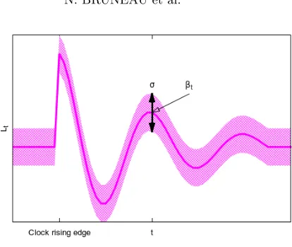
Definition 2. Let us now define a modulated trace as a trace in which each time sample can be expressed as a modulation of a model (static in time) plus an inde-pendent noisy part:
L= (βtf(Z) +Nt)t∈T =f(Z)β+ (Nt)t∈T , (3)
where β is a vector in RT and each Nt is drawn from an independent identical distribution N. In specific, the variance of the noise does not depend on the time samplet∈T.
This notion is illustrated in Fig. 1. In this figure, the pink curve represents the deterministic part of the signal, which is a damped oscillation due to the mismatch between the sensor and the leakage source. The pinkish area extending over the pink line represents thenoise noise. This figure1clearly shows that there are many samples which can be advantageously combined, in a view to increase the signal-to-noise ratio.
Theorem 1. In the case of modulated traces the solution of PCA is equivalent to maximizing the covariance (Eqn.(2)). More precisely, ifL= (βtf(Z) +Nt)t∈T then
α∈argmax kαk=1
Cov[L·α, f(Z)]2 ⇐⇒ α∈argmax kαk=1
Var[E[L|f(Z)]·α].
Fig. 1: Example of a modulated trace
Notice that, in Theorem 1, we consider that many vectors α can maximize the covariance: so, the return value of the argmax operator is a set.
In a particular case of Theorem1 we can explicitly describeα.
Lemma 1. If α and β are linearly dependent, we have:
β
kβk ∈argmaxkαk=1 Cov[L·α, f(Z)]
2 . (4)
Proof. The proof is given in Appendix B. ut
After projection into the new reduced space the covariance matrix will be zero everywhere except at (0,0). Moreover, all the variance should be contained in the first principal direction, thus, we do not need to take the other eigenvectors into consideration.
Asβ does not depend on a particular model we also maximize the covariance for wrong keys in the same proportion as the covariance for the good key. Thus we do not change the way we distinguish the good key from the wrong ones (the relative distinguishing margin is unchanged [25]). However, the dimensionality reduction leads to an improvement of the attack by increasing the signal-to-noise ratio (SNR). We define the SNR as the variance of the signal divided by the variance of the noise. This definition of SNR coincides with the Normalized Inter-Class Variance (NICV [5,4]).
Lemma 2. If the noise Nt is identically distributed (i.d.) for all t, then the noise is unchanged by any linear combination of unitary norm.
Proposition 3. If the noise Nt is i.d. for all t, then the signal-to-noise ratio is maximum after the projection:
max
t∈T Var[βtf(Z)]
Var[N] ≤ max
kαk=1Var[E[L|f(Z)]·α] Var[N] .
Proof. By definition of α we have max
t∈T Var[βtf(Z)]≤kmaxαk=1Var[E[L|f(Z)]·α].
Be-sides, by lemma2, the numerator of the SNR does not depend on our preprocessing,
since is satisfies kαk= 1. ut
Remark 4. In the case of modulated traces the PCA gives the solution of a matched-filter [14].
2.4 Covariance vector as a preprocessing method
In the general case when the model is not known or in the presence of noise, the variance may not only be contained in the first eigenvector [2]. Therefore, it may be useful to also take the other directions of the PCA into account. Note that, we still obtain an optimal function to reduce the dimensionality before conducting a CPA under the same leakage model assumption.
Proposition 4 (Covariance method).
Cov[Lt;f(Z)] k(Cov[Lt;f(Z)])t∈Tk
t∈T
∈argmax kαk=1
Cov[L·α, f(Z)]2
Proof. The proof is given in Appendix C. ut
So, the normalized covariance is the optimal preprocessing method to maximize the value of the covariance when using linear combinations of traces points. In the rest of this study we call this method the “covariance method” and the result the “covariance vector”.
Remark 5. Note that, the model of the actual leakage of the traces is not used in the proof of AppendixC. The results are therefore applicable for any leakage model such as the one presented in [10].
2.5 Discussion
on its own (see thebig picturein Fig.2); it can be seen as a generalization to higher-order attacks of [11]. Some other preprocessing tools have been proposed to reduce the dimensionality and enhance the quality of the CPA. The PCA [2] is a known way to preprocess the data to reduce the dimension and increase the efficiency of attacks. As defined in Sect.2.3, PCA is directly linked to the maximization problem, which is also underlined by our empirical results given in Sect. 3.
Oswald and Paar showed in [17] that the best linear combination (“best” in the sense of separating the highest peaks from the nearest rival) can be approached by numerical resolutions. The model presented in [11] is not totally applicable to our study case. If we are in the case of modulated traces, the expectation over each sample of the combined traces could be null. In this case the method presented is not directly suitable.
The point of this study is not to exhibit a better method for dimensionality reduction but to show that we can solve this problem in an easier way by using the vector of covariance.
Other preprocessing methods can be used before any dimensionality reduction such as reduction filtering using a Fourier or a Hartley transform [3]. However, when the transformation is linear and invertible, the covariance method applies in a strictly equivalent way. The next subsection clarifies this point on the example of the Fourier transform.
2.6 Time vs Frequency domains
Let L a signal in time domain, i.e., L = (Lt)t∈T. The representation of L in the frequency domain is the discrete Fourier transform F(L).
Definition 3 (Discrete Fourier transform). Let ı be a square root of −1 in C.
The discrete Fourier transform of L is a vector F(L) of same length, defined as F(L)f =Pt∈J1,TKLt·e−2πıf t/T, for allf in the interval J1, FK (whereF =T).
Proposition 4 can also be applied on F(L) instead of L. We then have the following Corollary.
Corollary 1 (Covariance method in the frequency domain).The covariance method in frequency domain yields covariance vectors equal to the Fourier transform of the covariance vectors in the time domain.
Proof. We have F(L) ·α = L· F(α), by interversion of the sums on f and t. Besides, Parseval’s theorem states that ||F(α)||2 = ||α||2. Thus, the application of
Proposition4onF(L) instead ofLyieldsF(α), whereαare the covariance vectors
LeakageL
α= ||cov(cov(LL;;ff((ZZ))))||
Correlation|ρ(L;f(Z))| Distinguishers:
Projection by linear combination (1’)
max k,t∈J1,T1K×J1,T2K
max
k |ρ(L·α;f(Z))| (0’)
(1’)
|ρ(Lt;f(Z))|
L·α
(scalar)
T1 T2
(1) (2)
t1 t2
1
1 t1
t2
t2
t1
(2’)
Fig. 2: Big picture of the “covariance method”. The usual 2O-CPA computes a cor-relation for each pair (t1, t2) of leakage (step (1)), and then searches for a maximum
over the keys and the time instances (step (2)). Our new method obtains a “covari-ance vector” (termed α) on a “learning device” (step (0’)), and then first projects the leakageLonα(step (1’)), before looking for the best key only while maximizing the distinguisher (step (2’)). Notice that the model f(Z) depends implicitly on the key guessk.
3 Empirical results
3.1 Implementation of the masking scheme
To evaluate these two methods we use the publicly available traces of the DPA contest v4 [23], which uses a first order low-entropy masking protection applied on AES called Rotating S-box Masking (RSM). In RSM only sixteen Substitution boxes (S-boxes) are used and all the sixteen outputs ofSubBytesare masked by a different mask. We take great in this paper to exploit second-order leakage (in particular, we avoid the first-order leakage identified by Moradi et al. [15]). Moreover, the same mask is used for the AddRoundKey operation where it is XORed to one plaintext byte P and in the SubBytes operation where it is XORed with the S-box output depending on another plaintext byte P0. As a consequence a bi-variate CPA can be built by combining these two leaks knowing P and P0. The leakage model in this case is given by:
f(Z) =E(wH(P ⊕M)−4)· wH(Sbox[P0⊕K]⊕M)−4
|P, P0, K, (5)
where P, P0, K are two bytes of the plaintext and a byte of the key respectively, together noted Z = (P, P0, K), and where wH(·) is the Hamming weight function and the expectation is taken overK. We denote this combination as (XOR, S-Boxes). Moreover, we also define another way to combine points in order to compensate the mask. As only sixteen different masks in RSM are used, also a link between the masks used at the output of the S-boxes exists. Accordingly, the combination of the outputs of two different S-boxes are not well balanced and we could consider an attack depending on two different S-Boxes which use two different masks. In this case the leakage model for the bi-variate CPA is:
f(Z) =E(wH(Sbox[P⊕K]⊕M)−4)· wH(Sbox[P0⊕K0]⊕M0)−4
|P, P0, K, K0.
(6)
In this equation, which we denote as (S-Boxes, S-Boxes),P andK(resp.P0 andK0) are the plaintext and key bytes entering the first (resp. the second) S-Box, andZ is a shortcut for the quadruple (P, P0, K, K0). We notice that there exists a deterministic link betweenM andM0;M andM0 belong to some subset{m0, m1, . . . , m15}ofF82.
We assume that M enters S-box 0≤i≤15 and M0 S-box 0≤i0 ≤15. Then when
M =moffset for some 0≤offset≤15, we have that M0 =moffset+i0−i mod 16.
3.2 Leakage analysis
We assume that the adversary is able to identify the area where the two operations leak during the “learning phase”. In order to analyze the leakage of the two opera-tions, we first calculate the covariance of the traces when the mask is known using 25000 measurements.
The covariance is computed for all key guessesK, where the wrong keys are plotted in grey and the correct key in red. Note that, as we target an XOR operation the maximum of the absolute value of the covariance is reached for two key guesses, namely the correct one and its opposite. It is quite clear, in Fig. 3a, that the traces are reasonably modulated (as per Def. 2); consequently, the relative distinguishing margin is constant over all the whole trace (as underlined in Sec.2.3). In the sequel, we use as leakage for the first sharewH(P⊕M)−4 instead ofwH(P⊕M⊕K)−4. As the second share is key-dependent, this choice allows us to restrict ourselves to one key search instead of two.
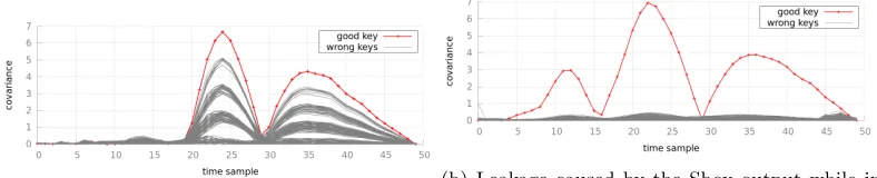
Figure 3b presents the covariance between the points where the output of an S-box leaks and the leakage model wH(Sbox[P0⊕K]⊕M)−4.
In both cases the mask leaks over several points; 50 samples represent less than 1 clock cycle. In this case the leakage is not uniformly spread over the points, thus it is reasonable to use a weighted sum to reduce the dimensionality of the data.
As the two leakages do not depend on the same operations their shapes are different. Interestingly, the distance between the correct key (red) and the next rival (grey) is much smaller in Figure3athan in Figure3b, Indeed the covariance plotted in Figure 3a is computed using a leakage depending on AddRoundKey, whereas the covariance plotted in Figure 3b is computed using a leakage caused by SubBytes. More precisely, the second plot corresponds to a time window when the value of the S-box output is moved during theShiftRows operation that followsSubBytes.
(a) Leakage caused byAddRoundKey
(b) Leakage caused by the Sbox output while in ShiftRows
Fig. 3: Covariance absolute value, for (a) XOR and (b) S-box
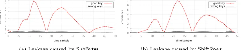
Figure 4a (resp. 4b) presents the covariance between the points where the out-put of an S-box leaks and the leakage model wH(Sbox[P ⊕K]⊕M)−4 (resp.
due to the SubBytes operations and the corresponding model. As looking-up and moving a byte are different operations, they leak differently.
(a) Leakage caused bySubBytes (b) Leakage caused byShiftRows
Fig. 4: Covariance absolute value, for (a) S-box and (b) S-box+ShiftRows
3.3 Experimental protocol
In this experiment we select two windows of 50 points corresponding to the leakage of the two shares. Then all possible pairs of points have been combined using the centered product function [18]. In all the experiments, the preprocessing method and the 2O-CPA are applied on these “combined” traces. We compare 2O-CPA with and without preprocessing.
We used the 50000 first traces of the DPA contest v4 for the learning phase and the remaining for the attack phase. To compute the success rate we repeated the experiment as many times as we could due to the restricted amount of traces.
Note that, several attacks using profiling or semi-profiling have been published in the Hall of Fame of the DPA contest v4. Most of these attacks are specially adapted to the vulnerabilities of the provided implementation or the particularities of RSM. However, our proposed preprocessing tools do not particularly target RSM, moreover, they are generic and could be applied to any masking scheme leaking two shares.
3.4 Comparison of the two preprocessing methods and classical second-order CPA
First of all, for the (XOR, S-Boxes) combination we see in Fig. 5 that the prepro-cessing improves the efficiency of the attacks. We need less than 200 measurements to reach 80% of success with the covariance or PCA preprocessing while we need more than 275 measurements for the classical 2O-CPA, which gives an improvement of 30%.
Fig. 5: Comparison between the classical second-order CPA and second-order CPA with preprocessing using (XOR, S-Boxes)
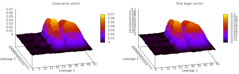
Fig. 6: Comparison between covariance vector and the first eigenvector
vector). The larger the value on the z-axis of Fig.6 and 8, the higher the contribu-tion (weight) of this point. The axes “leakage 1” and “leakage 2” represent the part depending on the two leakages of XOR (Fig.3a) and S-box (Fig.3b) operations in the combined traces. We can see in Figure 6 that the two methods highlight the same points of the combined traces and have the same shape (approximately the same values). Thus, the two methods give similar results in terms of success rate, which is confirmed by Figure5.
means that we are precisely in the framework of Theorem1: the display traces that are almost perfectly modulated by one static leakage model.
Fig. 7: Comparison between the classical second-order CPA and second-order CPA with preprocessing using (S-boxes, S-Boxes)
Fig. 8: Comparison between the covariance vector and the first eigenvector
(a) Standard deviation of 3 (b) Standard deviation of 5
Fig. 9: Comparison between 2O-CPA with preprocessing method and without in presence of Gaussian noise, with a standard deviation of 3 for (a) with a standard deviation of 5 for (b)
3.5 How is the preprocessing linked to the noise?
We have theoretically shown in Proposition3that the presented preprocessing meth-ods improve the SNR. We now empirically verify this results. In each point we add Gaussian noise to mimic real noisy measurements. We perform this experiment on the same points and with the same model as used for Figure5.
Figure 9a shows that using preprocessing methods improves second-order CPA in presence of noise. In this case we added Gaussian noise with a standard deviation of 3. The attacks after preprocessing need around 225 measurements to reach 80% of success whereas the 2O-CPA needs more than 550 measurements. Thus, prepro-cessing leads to a gain over 50%. As shown in Figure 5 the gain was close to 30% without noise.
In Figure 9b we can see that for Gaussian noise with a standard deviation of 5 the gain is more than 75%. Indeed the 2O-CPA after preprocessing needs around 250 traces reach 80% of success rate whereas for 2O-CPA 1000 measurements are not sufficient.
So this kind of preprocessing by dimensionality reduction is well designed against noisy implementation where the noise is not correlated with the time or the data.
4 On the fly preprocessing
esti-mate the covariance matrix for the PCA and the covariance vectors. However, the attacker might not always have this powerful tool.
As seen in Subsect.3.4 even for a small number of traces for the learning phase we have a significant improvement when we use preprocessing methods. We therefore evaluate these tools also as “on the fly” preprocessing methods.
4.1 Case study
We now model a less powerful attacker who does not have a “learning device” and estimates the value of the coefficient of the linear transformation directly on the traces used for the attack. Because the key is unknown the preprocessing method has to be computed for each key hypothesis. Finally, the adversary applies the covariance between the transformed data and the model depending on the key hypothesis. In this experiment we use the 10000 first traces of the DPA contest to compute the success rate which results in 25 repetitions.
4.2 Empirical results
Figure 10a illustrates the success rate after preprocessing for different sizes of the learning set for PCA (green) and the covariance vector (red). One can observe that the covariance method performs better than PCA when a low number of traces is used during the learning phase, accordingly, this method is a good choice as a “on the fly” preprocessing method. The reason why the PCA method needs more measurements for the learning than the covariance method to reach its maximum efficiency during the attack phase could be the fact that the covariance matrix (see the termtXX in Def. 1) needs more traces to be well estimated.
Figure 10b shows that with the “on the fly” preprocessing we can perform 2O-CPA using 225 measurements. This represents a gain of 18% compared to raw (sample-wise) 2O-CPA.
5 Conclusions and Perspectives
In this article we presented the covariance method as an optimal preprocessing method for second-order CPA. By using all possible leakage points our method improves the efficiency of the attacks and as the number of combined leakage points grow quadratically, thus our preprocessing method is well adapted for bi-variate CPA. We further theoretically linked the PCA to the problem of maximization of the covariance. We demonstrated theoretically the result of the covariance method to be the optimal linear combination for maximizing the covariance and underlined empirically that this method improves the result ofbi-variate CPA.
(a) Comparison between covariance and PCA de-pending on the size of the learning base
(b) Comparison between covariance in line pre-processing and 2O-CPA
Fig. 10: Evaluation of inline preprocessing methods
leaking points is important. This is partly explained by the fact the optimal covari-ance considers all the relevant sampling points, whereas the 2O-CPA considers only the best pair of samples and does not exploit the other interesting pairs.
We have also shown that the optimal covariance method is more efficient than PCA when the learning phase is performed on the fly. All the results have been vali-dated by experiences on real traces corresponding to masking implementation of the DPA contest v4. As a consequence dimensionality reduction by linear combination is well adapted to the case of multi-variate CPA. Moreover, the higher the order of masking, the more efficient the attack after preprocessing.
In our future work we will extend the previous results on other implementations which are less favorable to attacker, e.g., with more noise. Also we plan to compare the method presented in this article and the method presented in [11] in these cases. We will additionally apply these methods on different masking scheme especially on higher-order masking schemes.
References
1. C´edric Archambeau, ´Eric Peeters, Fran¸cois-Xavier Standaert, and Jean-Jacques Quisquater. Template Attacks in Principal Subspaces. In CHES, volume 4249 of LNCS, pages 1–14. Springer, October 10-13 2006. Yokohama, Japan.
2. Lejla Batina, Jip Hogenboom, and Jasper G. J. van Woudenberg. Getting more from pca: First results of using principal component analysis for extensive power analysis. In Dunkelman [8], pages 383–397.
3. Pierre Belgarric, Shivam Bhasin, Nicolas Bruneau, Jean-Luc Danger, Nicolas Debande, Sylvain Guilley, Annelie Heuser, Zakaria Najm, and Olivier Rioul. Time-Frequency Analysis for Second-Order Attacks. In Aur´elien Francillon and Pankaj Rohatgi, editors,CARDIS, volume 8419 of
4. Shivam Bhasin, Jean-Luc Danger, Sylvain Guilley, and Zakaria Najm. NICV: Normalized Inter-Class Variance for Detection of Side-Channel Leakage. InInternational Symposium on Electromagnetic Compatibility” (EMC ’14 / Tokyo). IEEE, May 12-16 2014. Session OS09: EM Information Leakage. Hitotsubashi Hall (National Center of Sciences), Chiyoda, Tokyo, Japan. 5. Shivam Bhasin, Jean-Luc Danger, Sylvain Guilley, and Zakaria Najm. Side-channel Leakage and Trace Compression Using Normalized Inter-class Variance. In Proceedings of the Third Workshop on Hardware and Architectural Support for Security and Privacy, HASP ’14, pages 7:1–7:9, New York, NY, USA, 2014. ACM.
6. ´Eric Brier, Christophe Clavier, and Francis Olivier. Correlation Power Analysis with a Leakage Model. InCHES, volume 3156 ofLNCS, pages 16–29. Springer, August 11–13 2004. Cambridge, MA, USA.
7. Suresh Chari, Josyula R. Rao, and Pankaj Rohatgi. Template Attacks. InCHES, volume 2523 ofLNCS, pages 13–28. Springer, August 2002. San Francisco Bay (Redwood City), USA. 8. Orr Dunkelman, editor. Topics in Cryptology - CT-RSA 2012 - The Cryptographers’ Track at
the RSA Conference 2012, San Francisco, CA, USA, February 27 - March 2, 2012. Proceedings, volume 7178 ofLecture Notes in Computer Science. Springer, 2012.
9. Louis Goubin and Jacques Patarin. DES and Differential Power Analysis. The “Duplication” Method. InCHES, LNCS, pages 158–172. Springer, Aug 1999. Worcester, MA, USA. 10. Suvadeep Hajra and Debdeep Mukhopadhyay. Pushing the limit of non-profiling dpa using
multivariate leakage model. IACR Cryptology ePrint Archive, 2013:849, 2013.
11. Suvadeep Hajra and Debdeep Mukhopadhyay. On the Optimal Pre-processing for Non-profiling Differential Power Analysis. InCOSADE, Lecture Notes in Computer Science. Springer, April 14-15 2014. Paris, France.
12. Ian T. Jolliffe. Principal Component Analysis. Springer Series in Statistics, 2002. ISBN: 0387954422.
13. Paul C. Kocher, Joshua Jaffe, and Benjamin Jun. Differential Power Analysis. InProceedings of CRYPTO’99, volume 1666 ofLNCS, pages 388–397. Springer-Verlag, 1999.
14. Thomas S. Messerges, Ezzy A. Dabbish, and Robert H. Sloan. Investigations of Power Analysis Attacks on Smartcards. InUSENIX — Smartcard’99, pages 151–162, May 10–11 1999. Chicago, Illinois, USA.
15. Amir Moradi, Sylvain Guilley, and Annelie Heuser. Detecting Hidden Leakages. In Ioana Boureanu, Philippe Owesarski, and Serge Vaudenay, editors,ACNS, volume 8479. Springer, June 10-13 2014. 12th International Conference on Applied Cryptography and Network Secu-rity, Lausanne, Switzerland.
16. Svetla Nikova, Vincent Rijmen, and Martin Schl¨affer. Secure hardware implementation of nonlinear functions in the presence of glitches. J. Cryptology, 24(2):292–321, 2011.
17. David Oswald and Christof Paar. Improving side-channel analysis with optimal linear trans-forms. In Stefan Mangard, editor,CARDIS, volume 7771 ofLecture Notes in Computer Science, pages 219–233. Springer, 2012.
18. Emmanuel Prouff, Matthieu Rivain, and R´egis Bevan. Statistical Analysis of Second Order Differential Power Analysis. IEEE Trans. Computers, 58(6):799–811, 2009.
19. Werner Schindler, Kerstin Lemke, and Christof Paar. A Stochastic Model for Differential Side Channel Cryptanalysis. In LNCS, editor,CHES, volume 3659 ofLNCS, pages 30–46. Springer, Sept 2005. Edinburgh, Scotland, UK.
20. Youssef Souissi, Shivam Bhasin, Sylvain Guilley, Maxime Nassar, and Jean-Luc Danger. To-wards Different Flavors of Combined Side Channel Attacks. In Dunkelman [8], pages 245–259. 21. Youssef Souissi, Maxime Nassar, Sylvain Guilley, Jean-Luc Danger, and Florent Flament. First Principal Components Analysis: A New Side Channel Distinguisher. In Kyung Hyune Rhee and DaeHun Nyang, editors,ICISC, volume 6829 ofLecture Notes in Computer Science, pages 407–419. Springer, 2010.
5154 of Lecture Notes in Computer Science, pages 411–425. Springer, August 10–13 2008. Washington, D.C., USA.
23. TELECOM ParisTech SEN research group. DPA Contest (4th edition), 2013–2014. http: //www.DPAcontest.org/v4/.
24. Jason Waddle and David Wagner. Towards Efficient Second-Order Power Analysis. InCHES, volume 3156 ofLNCS, pages 1–15. Springer, 2004. Cambridge, MA, USA.
25. Carolyn Whitnall and Elisabeth Oswald. A Fair Evaluation Framework for Comparing Side-Channel Distinguishers. J. Cryptographic Engineering, 1(2):145–160, 2011.
A Proof of Theorem 1
Proof. On the one side we have
Cov[L·α, f(Z)] = (Cov[St+Nt, f(Z)])t∈T ·α
= (Cov[St, f(Z)])t∈T ·α = (E[Stf(Z)])t∈T ·α .
The other side yields Var[E[L|f(Z)]·α] = Var(St)t∈T ·α
. Now if St = βtf(Z), then we have for both sides
Cov[L·α;f(Z)]2 = (α·β)2Ef(Z)22,
Var[E[L|f(Z)]·α] =Var[(α·β)f(Z)] = (α·β)2Ef(Z)2,
which proves equivalence. ut
B Proof of Lemma 1
Proof.
argmax kαk=1
Cov[L·α, f(Z)]2 = argmax kαk=1
(α·β)2Ef(Z)22
= argmax kαk=1
(α·β)2, because Ef(Z)22 >0.
By the Cauchy-Schwarz theorem, we have: (α·β)2 6kαk2×kβk2,where equality holds if and only if α and β are linearly dependent, i.e., α = λβ. Accordingly, if kαk= 1 we have λ= k1βk, which gives us the required solution. ut
C Proof of Proposition 4
Proof. We have
Similar to the proof of Lemma1, we use the Cauchy-Schwarz inequality. In partic-ular,
(Cov[Lt;f(Z)])t∈T ·α
2
6kαk2× k(Cov[Lt;f(Z)])t∈Tk2. We have the equality,
(Cov[Lt;f(Z)])t∈T ·α2=kαk2× k(Cov[Lt;f(Z)])t∈Tk2, if and only if α=λ(Cov[Lt;f(Z)])t∈T.
So, if kαk= 1 we have λ= k(Cov[L 1