..
VICTORIA UNIVERSITY
OF TECHNOLOGY
DEPARTMENT OF
MATHEMATICS, COMPUTING
AND OPERATIONS RESEARCH
THE USE OF A CLASS OF FOLDOVER DESIGN AS SEARCH DESIGNS
Neil T. Diamond
(1EQRM1)
September 1990
TECHNICAL REPORT
DEPT OF MCOR
FOOTSCRAY INSTITUTE OF TECHNOLOGY VICTORIA UNIVERSITY OF TECHNOLOGY BALLARAT ROAD (P 0 BOX 64), FOOTSCRAY
VICTORIA, AUSTRALIA 3011 TELEPHONE (03) 688-4249/4225
DESIGN AS SEARCH DESIGNS
Neil T. Diamond
(1EQRM1)
September
1990Efficiency, Quality and Reliability
Management Centre
This paper has been accepted for publication
inTHE USE OF A CLASS OF FOLDOVER DESIGNS AS SEARCH DESIGNS
NEIL T. DIAMOND
It is shown that a class of two-level nononhogonal resolution IV designs with n
factors are strongly resolvable search designs when k, the maximum number of
two-factor interactions thought possible, equals one; weakly resolvable when k = 2
except when the number of factors is 6; and may not be weakly resolvable
when k~ 3.
Key words: Fractional factorial designs; nononhogonal designs; resolution N
designs; search designs.
1. Introduction.
Resolution N designs allow the estimation of all main effects clear of the bias due to non-zero two-factor interactions. The most common designs used in
practice and discussed in the literature are onhogonal and for these designs the
two-factor interactions are aliased with each other.
Margolin ( 1969) has discussed the use of nononhogonal resolution
N
designs involving n two-level factors in 2n runs which for most values of n
would involve fewer runs with a small sacrifice in the efficiency of the
estimation of the main effects. However, as is shown below, these
non-onhogonal designs may allow the search and estimation of a small number of
non-zero two-factor interactions when considered as search designs.
2. Search Designs.
Srivastava (1975) pointed out that the factorial effects in an experiment can be
divided into three categories:
(i) effects that we are sure are negligible,
(ii) effects that we want to estimate, and
(iii) the remaining effects, most of which are negligible, but a few of which
Designs which provide estimates of all effects of type (ii) and enable a search
for the non-negligible effects from type (iii), on the assumption that there is no
error, are called strongly resolvable search designs. If the search can only be
carried out for some values of the non-zero interactions then the design is
called weakly resolvable.
Srivastava showed that a necessary and sufficient condition for a 2° factorial
design to be strongly resolvable when the maximum number of non-negligible
effects is k, is that every submatrix of the design matrix consisting of all the
columns corresponding to the effects of type (ii) and 2k of the columns
corresponding to the effects of type (iii) is of full rank.
3. Modified One Factor at'a Time Foldover Designs.
The class of resolution IV designs considered here is generated by using the
foldover theorem established by Box and Wilson (1951,p.35) who showed
that folding over any resolution III design involving (n-1) factors results in a
resolution IV design involving n factors. Talce, for example, the case when
n = 5. The classical one factor at a time design involving 4 factors, A, B, C
and D, is a resolution III design and consists of the runs ( (1), a, b, c, d}.
Replacing the first run of this design, where all the factors are at their low
level, by the run where all the factors are at their high level, in this case
abed, the design (abed, a, b, c, d} is obtained. John (1971, p172) has
shown that this construction leads to a design also of resolution
m
which isalways more efficient than the one factor at a time design for all values of n.
We will call such a design a modified one factor at a time design.
The modified one factor at a time foldover design consists of the modified one
factor at a time design and the foldover of that design, with an additional
factor incorporated set at its low level in the modified one factor at a time
design and at its high level in the foldover. With n =
5
the design is given bythe runs (abed, a, b, c, d, e, bcde, acde, abde, abce}. In fact, for all values
-3-It is easy to show that the variances of the main effect estimates in these
designs are given by (n2 - 5n + 8)/[2(n - 2)2]cr2. We can compare these
values to those given in Table 2 of Margolin's paper where the main effect
variances of the most efficient non-orthogonal resolution IV designs given
in the literature are tabulated. It needs to be stressed, however, that since
Margolin defines an effect of a factor A as half the difference between the
average response at the high level of A and the average response at the low
level of A, which is one half the usually defined A effect, Margolin's
variances need to be multiplied by four for a proper comparison. Making this
comparison it can be seen that the modified one factor at a time foldover
designs appear to be quite efficient when the number of factors is between 3
and 7. For n = 3, 5 and 7 the effect variances match the values presented by
Margolin while for n =
6
the effect variance for the design is 0.4375cr2which is only slightly higher than the tabulated value of 0.4cr2 . The case
when n = 4 is in fact the orthogonal 24-1 design with defining contrast
I= - ABCD which gives main effect estimates with 100% efficiency.
Since many industrial experiments do involve between 3 and 7 factors
an examination of these designs appears to be worthwhile.
However as the number of factors increases it should be noted that the designs
generated by folding over the resolution III designs given by Yang
(1966,1968) become increasingly more efficient than the designs
considered in this paper. The Yang foldovers have effect variances of
cr2
I
(2n - 2) for n = 2 (mod 4). Research on the use of the Yang foldovers assearch designs is currently in progress.
4. Searching For Non-negligible Two-factor Interactions.
For the modified one factor at a time foldover designs, with the assumption
that all three-factor and higher interactions are negligible, the design matrix is
of the form
x
= [:u
-U
where 1(nx1) = (1, 1, ... 1)', U (n x n) has l's on the diagonal and -l's
elsewhere and V denotes the matrix of the n(n - 1)/2 two-factor interaction
effects where the column corresponding to the interaction between the ith and
W e want to estimate the mean and the main effects and search over and
estimate the non-zero two factor interactions. To show that the design is of
resolving power k the rank of all matrices Y, consisting of the first (n + 1)
columns of X and 2k of the last n(n - 1)/2 columns of X, must be (n+ 1 +2k).
However, Webb (1968) has shown that the columns corresponding to the
main effects in any resolution IV design are linearly independent of one
another, and are orthogonal to, and therefo~e linearly independent of, the
columns corresponding to the mean and the two-factor interactions. We can
also centre the columns corresponding to the two-factor interactions to make
them orthogonal to the mean and hence we only have to show that every 2k
columns of then x [n(n-1)/2] matrix W
=
V - [(n-4)/n]J have full rank, whereJ
is then x [n(n-1)/2] matrix whose every element is I.The column of W corresponding to the interaction between the ith andjth factors, J3ij' takesthe values (4-2n)/n in the ith andjth rows and 4/n elsewhere.
It turns out that in order to determine whether a set of the J3 . .'s is linearly lJ
independent or not it is very useful to form the columns a ..
=
(2/n) - 0.5{3 ... ~ ~
which take the values 1 in the ith and jth rows and 0 elsewhere. The matrix of
the
a ..
corresponding to a set of 2k two-factor interactions is in fact anlj
incidence matrix of a graph with n vertices and 2k edges. Each vertex of the graph corresponds to one of the runs a, b, c, .... , and an edge between two
vertices is present if the interaction involving the same letters as the vertices is in the set. In addition a linear combination of the a.. say :EL. c1.J. a .. can be
lJ lJ
represented as a weighted graph or network, where the weight cij is assigned
to the edge corresponding to cxif Figure 1 shows for n = 5 the graph and
network corresponding to the set of two factor interactions {AB, AC, BD,
CD} and the linear combination (c12a12
+
c13a13+
c24
~+ ~~4
> respectively.Figure 1: Graph corresponding to {AB, AC, BO, CD} and Network corresponding to c12 cx12 + c13 cx13 + c24 cx24 + c34 ~ for n
=
5.e
•
c r - - T d
al---lb
e
•
C:34c 1 3 c l l d c 2 4
aL--'b
-5-Since the a .. take the values 1 lJ in the ith and jth rows and 0 elsewhere, the result of the above linear combination will be (c12+c13• c12+c24, c13+c34,
c24+c34, 0)', that is each element of the vector can be obtained by simply summing the weights of the edges incident with the corresponding vertex. This method of representing a linear combination gives a very easy way of checking whether the columns associated with a set of interactions are
linearly dependent since, as is shown below, a linear combination of the
J3 .
.'s islJ
zero if and only if a set of weights can be found so that the sums of the weights at each of the vertices are the same, that is LL c .. a .. = (x, x, ... , x)'
lJ lJ
for some real x. To prove the if part assume LL cij aij = (x, x, ... , x)'.
Then LL c1.J. (2/n - 0.5
J3
.
.
)
=
(x, x, ... , x)' and hence LL c ..j3
.
.
= (
4ll,lj lJ lJ
ciJn - 2x, ... , 4LL ciJn - 2x)'. But LL cij = nx/2 since the weights incident to every vertex add to x, there are n vertices and every edge is incident to two vertices. Hence LL
c ..
J3
..
= (0, 0, .. , 0)'. To prove the only if part assumelJ lJ
LL cijj3ij = (0, 0, ... , 0)'. Hence LL cij (4/n - 2aij) = (0, 0, ... 0)' and therefore LL a .. c .. = (x, ... , x)' with x = 2 l l c-/n. This is a very useful
lJ lJ 1
result that allows the determination of the linear dependence or independence of a set of interaction columns via the examination of the associated graph.
4.1 k
=
1.To show that the designs are strongly resolvable when k = 1 all the possible graphs with n vertices and 2 edges need only be considered. Since these designs are symmetric in each of the factors, in the sense that interchange of factor labels does not alter the design, it is only necessary to consider
-6-Since the number of graphs with 4 vertices and 2 edges is 2, see for
example Harary (1972, p.214), there are only two cases to consider which are
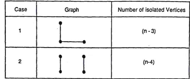
given on p.215 of Harary and summarised in Table 1.
Table 1: All graphs with n vertices and 2 edges
Case Graph Number of isolated Vertices
1
L
(n -3)2
I
I
(n-4)It is clearly not possible to assign non-zero weights to the edges so that the
sums of the weights at each of the vertices are the same except when n = 4.
Searching for at most one non-zero interaction is thus possible apart from
the case when n = 4 corresponding to the orthogonal 24· 1 design.
4.2 k=2.
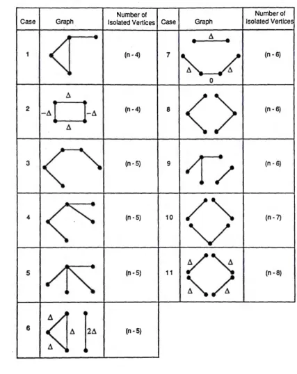
All the possible unlabelled graphs with n vertices and 4 edges need to be considered where n ~ 5, since there are at most 3 edges when n = 3 and the case n = 4 corresponds to the standard orthogonal design. Again from p. 215
of Harary the number of cases to consider is 11. The first 9 cases are given
on p. 218 of Harary and these together with the last two cases, found using
trial and error, are summarised in Table 2 with weights assigned to the edges
Table 2: All graphs with n vertices and 4 edges.
Number of Number of
Case Graph Isolated Vertices Case Graph Isolated Vertices
- .1
<.
-
•
•
1 (n • 4) 7
~
(n • 6)I
0
.1
<>
2
-"D"
(n • 4) 8 (n - 6)I
.1
'
-
-3
"'.
!
(n • 5) 9i
~/
(n -6)-
-/"'.
-' I
4 (n - 5) 10 (n. 7)
I
v
5
~
(n ·5) 11y~
(n -8)~~
~t.121>
I
-7-Case 2 is dependent for all values of n. -7-Cases 6, 7 and 11 are dependent only for n = 5,
6
and 8 respectively. All the other cases are independent The dependent cases can be used to show when searching for at most twonon-zero interactions is not possible.
For example from case 2 with n = 5 we can see that (Aa
12 - ila13 - 6~
+
A~) = (0, 0, ... , 0)' and also (Aa12 - Aa13 - Acx25
+
A°'J5) =(0, 0, ... , 0)', for arbitrary 6, and therefore 6~
12
- 6~13
- A~24
+
A~34
=A~
12
- A~13
- A~25
+
A~35
= (0, 0, ... , 0)'. If we consider the case where the interaction effects are AB= 6 and AC= -Ll, all other interactions beingzero, then the component of the observation vector orthogonal to the mean
and main effects is given by 6~
12
- 6~13
= A~24
- 6~34
= A~25
- A~35
and therefore the true Model {AB, AC}, with AB= A and AC= -6, cannotbe distinguished from the false models {BD, CD}, with BD =A
and CD= - A, and {BE, CE}, with BE= A and CE= - A, on the basis of the
data.
As another example, from case 6 with n = 5, we can see that (Aa
12
+
Aa13+
.!la23+
2.!la45) = (26, 26, ... , 26)' and therefore (A~12
+
6~13
+
6~23
+
2A~45
) = (0, 0, ... , 0)'. If we consider the case where the interaction effects are AB = A and AC = A, all other interactions being zero, then thecomponent of the observation vector orthogonal to the mean and main effects
is given by 6~
12
+
6~13
= -6~23
- 2A~45
and therefore the true model {AB, AC} , with AB= 6 and AC= A, cannot be distinguished from the
-8-A complete examination of Table 2 shows that searching is not possible only
for the following true models:
1. The true model consists of two interactions with one letter in
common where:
(a) the interaction effects are equal in magnitude but opposite in sign,
or (b) the interaction effects are equal and n = 5.
or
2.
The true model consists of two interactions with no letters in common where:(a) the interaction effects are equal,
or (b) one of the interaction effects is twice the other interaction effect and
n=5.
or
3. The true model consists of only one interaction and n
=
6:In the latter case, which follows from case 7 of Table 2, the design is not even weakly resolvable, since if the true model is {AB} with AB= A, say, then the
true model cannot be separated from the model {CD, EF}, with CD
= -
A
and EF= -
A, and other models under an interchange of letters, irrespective of thevalue of A. It should be noted that case 7 is only dependent when a zero
weight is assigned to the edge specified in Table 2 and this is equivalent to
dropping the corresponding interaction from the Model being considered.
4.3 k = 3.
Examination of case 2 of Table 2 shows that for any value of n the design may
not be even weakly resolvable, for if the true model consists of one
interaction, say AB, with value A then it is not possible to separate it from the
-9-5. Conclusion.
The results of the previous section show that if k =l, then the designs
considered here are perfectly satisfactory, at least in the error-free case.
If k = 2 and n "#. 6 then the designs will be satisfactory unless the parameter
values of the two factor interactions take on certain values, in which case an
augmenting design, along the lines of those used by Daniel (1962,1976
Chapter 14) for orthogonal resolution IV designs, would need to be run. The main advantage of these designs over the usual orthogonal fractional replicates
is that on many occasions no augmenting designs will be required.
If k = 2, n = 6 and, if only one interaction is non-zero, augmenting
will be required irrespective of the value of the interaction effect. If two interactions are non-zero augmenting will only be required when the
interactions take on certain values. The case when k = 3 is similar in that when only one interaction is non-zero augmenting will be required but if two or three interactions are non-zero augmenting will only be required
for certain parameter values.
These results indicate that the designs considered here should not be used when k
=
2 and n=
6 or when k=
3 since their major advantage over theorthogonal designs may be absent.
Finally, the performance of the designs when error is present and the design
of augmenting trials, when required, will be reported in a subsequent paper.
Acknowledgements:
This work was completed as part fulfilment of the author's Ph.D currently in
progress in the Deparr;ment of Statistics at the University of Melbourne.
I would like to thank my supervisor, Dr. Ken Sharpe, for his help and
-10-References:
Box, G.E.P. and K.B. Wilson. (1951), On the experimental attainment of optimal conditions,
J.
Roy. Stat. Soc., Series B, 13, 1 - 45Daniel, C. (1962), Sequence of fractional replicates in the 2 p-q series, J. Am. Stat. Soc., 58, 403 - 429
Daniel, C. (1976), Applications of Statistics to Industrial Experimentation, New York :_John Wiley & Sons
Harary, F. (1972), Graph Theory. Reading, Massachusetts: Addison - Wesley
John, P.W.M. (1971), Statistical Design and Analysis of Experiments, New York : MacMillan Co.
Margolin, B.H. (1969), Results on factorial designs of Resolution IV for the 2n and 2n 3m Series, Technometrics, 11, No. 3, 431 - 444
Srivastava, J.N. (1975) Designs for searching non-negligible effects, in J.N. Srivastava, ed. A Survey of Statistical Design and Linear Models, North-Holland Publishing Company.
Webb, S. (1968), Non-orthogonal designs of even resolution, Technometrics, 10, No.2, 291-299.
Yang, C.H. (1966), Some designs for maximal (+1,-1)- detenninant of order n = 2 (mod 4), Mathematics of Computation, 20, 147-148. Yang, C.H. ( 1968), On designs of maximal (