Numerical modeling using an elastoplastic-adhesive
discrete element code for simulating hillslope debris flows
and calibration against field experiments
Adel Albaba1, Massimiliano Schwarz1, Corinna Wendeler2, Bernard Loup3, and Luuk Dorren1 1School of Agricultural, Forest and Food Science HAFL, Bern University of Applied Sciences, Länggasse 85, 3052 Zollikofen, Switzerland
2Geobrugg Protection Systems, Aachstrasse 11, 8590 Romanshorn, Switzerland
3Federal Office for the Environment (FOEN), Papiermühlestrasse 172, 3063 Ittigen, Switzerland Correspondence:Adel Albaba ([email protected])
Received: 16 October 2018 – Discussion started: 28 November 2018
Revised: 4 August 2019 – Accepted: 9 September 2019 – Published: 30 October 2019
Abstract. This paper presents a discrete-element-based elastoplastic-adhesive model which is adapted and tested for producing hillslope debris flows. The numerical model pro-duces three phases of particle contacts: elastic, plastic and adhesive. A parametric study was conducted investigating the effect of model parameters and inclination angle on flow height, velocity and pressure, in order to define the most sen-sitive parameters to calibrate. The model capabilities of sim-ulating different types of cohesive granular flows were tested with different ranges of flow velocities and heights. The ba-sic model parameters, the microscopic basal friction (φb) and ratio between stiffness parameters√k1/k2, were calibrated using field experiments of hillslope debris flows impacting a pressure-measuring sensor. Simulations of 50 m3of material were carried out on a channelized surface that is 41 m long and 8 m wide. The calibration process was based on measure-ments of flow height, flow velocity and the pressure applied to a sensor. Results of the numerical model matched those of the field data in terms of pressure and flow velocity well while less agreement was observed for flow height. Those discrepancies in results were due in part to the deposition of material in the field test, which is not reproducible in the model. Results of best-fit model parameters against selected experimental tests suggested that a link might exist between the model parametersφband
√
k1/k2and the initial condi-tions of the tested granular material (bulk density and wa-ter and fine contents). The good performance of the model against the full-scale field experiments encourages further investigation by conducting lab-scale experiments with
de-tailed variation in water and fine content to better understand their link to the model’s parameters.
1 Introduction
initial slope failure (Jibson, 1995; Schwarz et al., 2010; Oli-vares and Picarelli, 2003; Klubertanz et al., 2009; Shen et al., 2017), (ii) the transformation from a sliding block into a de-formed flowing mass (Iverson et al., 1997; Gabet and Mudd, 2006) and (iii) the kinematics of the flowing mass (veloc-ity, run-out, etc.). While both first aspects have been exten-sively investigated, the kinematics of hillslope debris flows have rarely been investigated.
Numerical modeling has been deployed as an effec-tive tool in simulating the behavior of shallow landslides and hillslope debris flows (Hungr, 1995; Montrasio and Valentino, 2016; Ran et al., 2018). For example, the software RAMMS:Hillslope was developed in the Swiss Federal Insti-tute for Forest, Snow and Landscape Research (WSL), based on a momentum balance using a Voellmy rheological model (Voellmy, 1955; Christen et al., 2010; Graf and McArdell, 2011). Another example is the mass-balance-based Flow-R model, which was developed in the University of Lausanne primarily for regional susceptibility assessments of debris flows (Horton et al., 2013). The model was successfully ap-plied to different case studies in various countries with vari-able data quality. It was also found relevant to assess other natural hazards such as rockfall, snow avalanches and floods. The basic concept of Flow-R was recently implemented and extended in a model developed at the HAFL called M-Flow, which has been tested for modeling hillslope debris flows (Scherer, 2016). The M-Flow model is fairly simple and only accounts for the mass distribution of the flowing mass ac-cording to the terrain, without in-depth investigation of the physical aspects of hillslope debris flows. However, the first preliminary tests using M-Flow to reproduce the propagation and impact pressures of real hillslope debris flow events gave promising results.
Discrete element simulations were also used to investi-gate flowing characteristics and impact pressures of granular flows down inclines (Teufelsbauer et al., 2009, 2011; Albaba et al., 2015; Wu et al., 2016; Shen et al., 2018). Parameters such as flow velocity, flow height and impact pressure were characterized in these simulations at different sections with in-detail investigation. Results of these simulations were of-ten compared to depth-averaged hydrodynamic models con-cerning the impacting pressure of these flows on rigid barri-ers (Faug, 2015; Albaba et al., 2018). Moreover, paramet-ric studies investigating the effect of inclination angles of the chute and the barrier on flow behavior and impact pres-sure were also carried out (Albaba, 2015). Although these simulations agreed well with the proposed theory concern-ing the impact, they were mainly carried out for dry granular flows with no consideration of fluid presence. Such presence would change the flow characteristics and the time history of its applied pressure (Vollmöller, 2004; Kattel et al., 2018). Other models based on the discrete element method (DEM) accounted for the presence of fluid by coupling a DEM with either a LBM (lattice Boltzmann method) or a CFD (compu-tational fluid dynamics) solver (Leonardi et al., 2016; Ding
and Xu, 2018). Such models were promising for theoreti-cal research questions but are computationally expensive for practical use in the daily practice of hillslope debris flow haz-ard assessment.
In addition to numerical modeling, lab, medium and full-scale experiments were carried out to investigate the flowing mass behavior of debris flows and their impact on rigid ob-jects. For instance, Hürlimann et al. (2015) set up a 7.5 m long experimental chute in which different samples with dif-ferent grain size distributions, water contents and volumes were tested. It was found that increasing water content, even by a small amount, would greatly increase the run-out dis-tance (exponential relationship). The increase in clay content resulted in a decrease in the run-out distance. In addition, a proportional relationship was observed between the run-out distance and the volume, although the effect was rather small. An intermediate-scale flume for testing debris flow was built by the United States Geological Survey (USGS) and is 95 m long, 2 m wide and 1.2 m deep (Iverson and LaHusen, 1993). The majority of its length slopes at 31◦while the re-maining part (7 m) gradually flattens to 2.5◦and it has a load-ing capacity of 20 m3 of granular material. The flume has been actively used since 1993 for investigating different as-pects of debris flow physics.
A full-scale hillslope debris flow experiment was carried out by Bugnion et al. (2012) by measuring the impact of 16 events of 50 m3in volume on two impact sensors. A 41 m long, 8 m wide channel was constructed on the side of a rock quarry in Switzerland. The advantage of such full-scale in-vestigation is that it allowed for detailed measurements that are usually overlooked in the post-analysis of previous land-slides and hillslope debris flows, especially those parame-ters that are very difficult to estimate for the post-analysis of events, mainly flow height, velocity and impact pressure.
All in all, although advancements have been achieved, the understanding of shallow landslides and hillslope debris flows is still lacking. Assessments of such natural hazards, unlike rockfalls and avalanches, are therefore mostly based on the experience of experts. In order to improve the hazard assessment of shallow landslides, new tools and methods are needed to calculate the disposition, the evolution and the run-out of hillslope debris flows on a slope for different situations (normal situation, severe precipitation, with and without for-est cover, etc.).
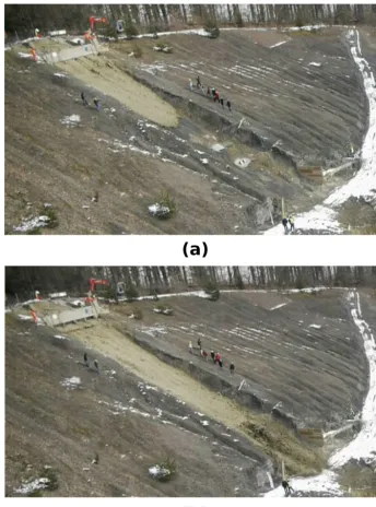
model-Figure 1.Aerial photo of several hillslope debris flow events in Switzerland following a severe rainfall event in summer 2005. Source: Federal Office for the Environment (FOEN).
ing 3-D real-scale experiments or back-calculating historical events of granular flows would be computationally possible. First, the field experimental data that are used to calibrate and validate the DEM are presented. Subsequently, the DEM is described in detail highlighting the key parameters to cali-brate. Next, a parametric study is presented investigating the effects of varying the model microscopic parameters in ad-dition to the mean particle diameter (d50) and channel incli-nation angle (α). A cross comparison between model results and experimental data is then carried out, with a special focus on flow height, flow velocity and the pressure applied by the flow on pressure-measuring sensors. Finally, the main results are discussed and conclusions are drawn.
2 Materials and methods
2.1 Field experiment of hillslope debris flow
A series of full-scale field experiments of hillslope debris flow were carried out between 2008 and 2010 at the Veltheim test site in the Canton Aargau in Switzerland (see Bugnion et al., 2012). The objectives of the experiments were to mea-sure the height and velocity of hillslope debris flows, as well as the pressure. A flexible barrier, which is widely used as a protection measure against many types of mass movements (Volkwein, 2005; Brighenti et al., 2013; Albaba et al., 2017), was installed downslope the channel and was intensively
in-strumented in order to measure the internal forces and de-formations developed in the barrier while being impacted by flows. In total, 16 tests were carried out, of which eight tests consisted of one release while the remaining eight tests con-sisted of successive releases, where the debris flows were leased successively without cleaning the channel. Each re-lease had a constant volume of 50 m3.
2.1.1 Geometry and material used
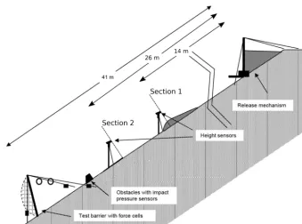
Figure 2.A schematic representation of the field experiment layout.
shortly after release (3 s after release) and after impacting the pressure sensors (6 s after release).
2.1.2 Measured parameters in the experiments
For each released flow, the flow height at sections 1 and 2 was measured using laser sensors. Sections 1 and 2 are located at distances 14 and 26 m, respectively, downstream from the starting reservoir, where distances are measured parallel to the slope as seen in Fig. 2. In addition, with two sensors in-stalled 30 cm apart at section 2, the velocity of the upper flow surface was derived using the discrete correlation function of the two height signals of the two sensors. The mean front ve-locity at section 2 was back-calculated using data related to flow arrival time and distance at sections 1 and 2. The pres-sure applied by the flowing material on the small and large plates was also measured and a filtering mechanism was ap-plied. The filtering of pressure values was applied in order to remove oscillations caused by hard contacts due to large grains that impact the sensors. It was applied by replacing each signal value by the mean value over an interval of 0.05 s. In Sect. 3.1, we investigated the possible relationships be-tween those measured parameters (flow velocity and height) in the experiments and water and fine content of released ma-terials. Previous studies of lab-scale experiments of hillslope debris flows showed that increasing water content had the largest positive change of the run-out distance, which might also indicate a possible increase in flowing velocity (Hürli-mann et al., 2015). In addition, a negative correlation was observed between clay content and run-out distance. Both of
those relations were found to be nonlinear. Run-out analysis is an important aspect of studying hillslope debris flows, but is out of the scope of this study, as it is not considered in the field experiment.
2.2 Discrete element simulations
The numerical simulation in this study was carried out using a discrete element method (DEM). Today the DEM is widely used for modeling granular media (Maurin et al., 2016; Pa-pachristos et al., 2017; Mede et al., 2018). It is particularly efficient for static and dynamic simulation of granular as-semblies where medium can be described at a microscopic scale. The method is based on an explicit finite difference scheme proposed by Cundall and Strack (1979). It applies for a collection of discrete bodies interacting with each other, governed by a contact law. Different contact forces can be considered in both the normal and the tangential direction. Calculations alternate between the application of Newton’s second law to particle motion and a force-displacement law for the particle interactions. In comparison with the finite el-ement method (FEM), the DEM makes large displacel-ements between elements easy to simulate and computationally in-expensive, which is useful when dealing with discontinuous problems in granular medium.
po-Figure 3.Screenshots of test 10: 3 s after release(a)and 6 s after release(b).
sitions and velocities of the particles. YADE contains the main components for the application of the DEM, which in-clude Newton’s law, time integration algorithms, damping methods, collision detection, data classes (storing informa-tion about bodies and interacinforma-tions) and command OpenGL methods for drawing popular geometries (Šmilauer et al., 2015).
2.2.1 Contact laws
In the numerical scheme, two possible types of interactions can take place. The first interaction type is the particle–wall
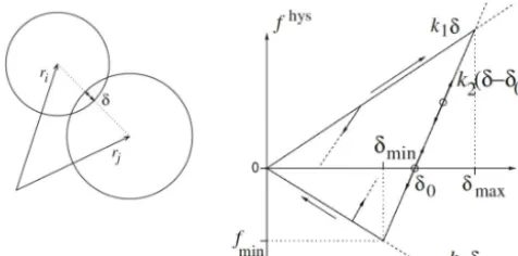
Figure 4.A schematic representation of the three phases of the con-tact law in normal direction.
and can be related to the restitution coefficient of granular materials.
The second type of interaction is particle–particle interac-tion, which describes the contact between a pair of spherical particles that are part of the granular flow. For this interac-tion, we implemented an elastoplastic-adhesive contact law in the YADE open-source code based on the work of Luding (2008) to simulate the behavior of a cohesive flow. A hysteric force between two interacting particlesFhysin the normal di-rection is calculated as follows (see also Fig. 4):
Fhys= ( k
1δ if k2(δ−δ0)>k1δ
k2(δ−δ0) if k1(δ) > k2(δ−δ0) >−kcδ −kcδ if −kcδ>k2(δ−δ0)
, (1)
wherek1,k2andkcare stiffness parameters for loading, un-loading and adhesive phases of contacts, respectively.δis the overlapping distance in the normal direction between the two particles.
When a contact between two particles is established, with particles pushing into each other, the hysteric force would start increasing linearly with the increase in the deforma-tionδalong the path ofk1. The maximum reached deforma-tion (δmax) will keep being updated as the deformation at the contact increases. Once unloading starts, the reached defor-mation would be temporarily saved as δmax and the force-deformation path would be followed on the line indicated by the stiffness parameterk2. In case of reloading, the path of k2 would be followed again until reaching the maximum recorded deformation δmax in which further loading would again follow the path ofk1. In case of unloading belowδ0, which represents the interception between thek2path and the deformation axis and is calculated asδ0=(1−k1/k2)δmax, an adhesive force would be activated, which is limited by the minimum force valuefmin= −kcδmin.
In addition to the hysteric force component, there is the classical viscous component of the forcefvisc(see for infor-mation Schwager and Poeschel, 2007), which is the prod-uct of the viscous damping coefficient (γn), that depends on the chosen value of the restitution coefficientn(taken equal to 0.3 as indicated by previous DEM studies of granular flows down inclines; Chanut et al., 2010; Albaba et al., 2015), and
the velocity in the normal direction (vn), which yields the following form of the interaction force in the normal direc-tionFn:
Fn= Fhys+γnvnn. (2)
The tangential component of the normal force is governed by the classical Mohr–Coulomb failure criterion as follows:
Ft= ktut
|ktut||Fn|tan8p if |ktut|>|Fn|tan8p
ktut otherwise
, (3)
wherektrepresents the tangential stiffness parameters,utis the tangential displacement and8pis the interparticle (mi-croscopic) friction angle.
The normal stiffness of the contact between two parti-cles (k1) is calculated as (Catalano et al., 2014)
k1=
2E1r1E2r2
E1r1+E2r2
, (4)
whereE1andE2are the elastic moduli of the first and second particles, respectively (both taken as 108Pa) andr
1andr2are the radii of the first and second particles, respectively. 2.2.2 Geometry and chosen parameters
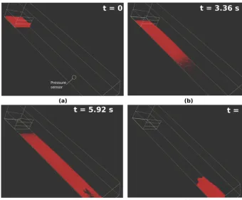
Figure 5.A series of screenshots during a DEM simulation withφb=30◦and
√
k1/k2=0.3: directly after opening the reservoir’s gate(a), att=3.36 s(b), att=5.92 s(c)and at the end of the simulation(d).
2.2.3 Mechanism of measuring parameters in YADE Since YADE is a discrete element code, parameters such as height, velocity and pressure were characterized at the par-ticle (micro)scale. In order to present those parameters on a macroscale that is comparable with those of the experimen-tal data, particle-scale parameters needed to be averaged in order to represent the flowing mass as a continuum medium. To compare the simulated mean front velocity with the ex-periment, the simulated flow arrival time was calculated at positions 1 and 2 and averaged over the distance between those two positions.
The maximum flow height at position 2 is a value that rep-resents the height of the main, coherent flowing body at that position. Firstly, a virtual box was used that was centered at position 2 and had a length 5×d50 and a width and height equal to those of the channel. Flow properties such as po-sition coordinates inx (in the direction of the flow),y (tra-verse the flow) andz(perpendicular to the base) as well as flowing velocity in the direction of the flow were recorded each 0.1 s for all particles within that box. Secondly, parti-cle height measurements at time periods between 25 % and 75 % of total impact duration were selected for each simu-lation, in order to exclude the disperse and dilute flow front and flow tail (Jiang and Towhata, 2013; Albaba et al., 2015), such as the ones seen in Fig. 5b. Thirdly, the 90 % cumulative frequency of flow height of particles within the box was
se-lected. The maximum flow height in YADE that is compared to the experiment was then the maximum value of those se-lected cumulative frequencies for all the samples that were collected each 0.1 s.
For the impacting pressure, a rigid wall in YADE was stalled at the same position where the large sensor was in-stalled during the experiments and with the same dimensions (Fig. 5a). Normal force Fn applied to the wall by flowing particles was calculated as follows:Fn=
n P
i=1
Fni, whereFni
is the normal force between a particleiand the wall, andnis the number of particles in contact with the wall at that mo-ment. The pressure was then calculated as the ratio between applied force and the sensor’s surface area.
2.2.4 Sensitivity analysis of DEM parameters
A sensitivity analysis study was carried out in order to in-vestigate the effect of change of different parameters on the model’s results concerning maximum flow height, mean flow front velocity and maximum applied pressure on the large plate. First, the effect of the filtering interval applied to the pressure signal was analyzed in order to use a unified filtering interval for all simulations. Afterwards, the effect of variation in each of the following parameters,φb,
√
k1/k2,kc,d50and
2.3 Comparison of DEM and experimental data To calibrate the DEM, only first releases of selected tests from the field experiment were considered in order to avoid the possible disturbance of measured parameters in the ex-periments due to the presence of deposits of previous releases (tests abbreviated asX.1 in Table 4 in Bugnion et al. (2012), whereXis the test number). In the current DEM, no material deposited on the inclined plane and thus the multiple releases would be difficult to reproduce. Seven tests from the experi-mental data were selected to be compared with the DEM re-sults. They are numbered with the same digits as in Bugnion et al. (2012). Table 1 summarizes the main material proper-ties of these tests and the measured parameters.
A series of simulations varying the parameter set (φb, √
k1/k2) were carried out. A range between 20 and 40◦ was selected for φb with a step-wise increase of 5◦ while √
k1/k2was varied between 0.3 and 0.45 with an increment of 0.03. Those ranges were selected based on preliminary model tests. Simulations withφband
√
k1/k2values that are outside the selected ranges were found to result in either very fast flows with very high impacting pressures or flows that would not slide along the channel. Afterwards, all carried-out simulations were compared with each selected experi-ment in order to find the best-fit in terms of maximum flow height at position 2 (Hmax), mean front velocity between po-sitions 1 and 2 (Vmean), and maximum applied pressure to the large sensor (Pmax). Results of pressures on smaller sen-sors were ignored because they were not measured for each test in Bugnion et al. (2012). In addition, in DEM simula-tions, the smaller the sensor, the more discrete in nature the force signal would be due to the presence of fewer particles per impact. A best-fit for each selected experimental test was determined as the lowest percentage (Rmin) of error for the three parameters as follows:
Rmin=min ∀i∈ns
p
(HDEM)i−HEXP HEXP
+ p
(VDEM)i−VEXP VEXP
+ p
(PDEM)i−PEXP PEXP
!
, (5)
wherensis the number of simulations.
After finding the best parameter set (φb, √k1/k2) for each experiment, possible relationships between these sets of parameters and initial condition of the granular samples (i.e., water and fine content) were investigated.
3 Results
3.1 Analysis of experimental data
For the seven selected experimental tests, a relationship seems to exist between the water content in the granular material prepared in the reservoir and the recorded mean
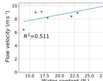
Figure 6.Relation between the water content of the granular ma-terial of selected experimental tests and the observed mean front velocity.
front velocity between sections 1 and 2 in the field exper-iment (Fig. 6). For example, test no. 16 had a water con-tent of 14 % and its recorded mean front velocity was found to be 6.4 m s−1. In addition, water contents between 16 % and 23 % had similar recorded front velocities ranging from 8.2 to 9.1 m s−1for test numbers 10 to 15. Test no. 9, which had the richest water content, had the highest mean front ve-locity of 10.2 m s−1. This observed increase in flow velocity with increasing water content could be due to the decrease in basal friction with the flowing material, which leads to higher flowing velocities. However, a best fit of the results might be better represented with a nonlinear equation in comparison with the regression line presented in Fig. 6, which is similar to observations of Hürlimann et al. (2015).
Another observation can be made regarding the relation-ship between the amount of fine content (silt and clay) in the prepared material in the reservoir and the maximum flow height recorded at position 2, which is found to be inversely proportional (Fig. 7). At low levels of fine content (21 %– 28 %), maximum flow heights were found to be between 0.33 and 0.40 m. A high increase in fine content, like in test no. 9, resulted in a drop in measured flow height to 0.29 m. However, such a relationship is not very evidently inverse. This is because for test no. 16, although the fine content was high (41 %), the recorded flow height was found to be larger than the average for all tests (0.37 m).
Simi-9 1790 28 48 0.29 10.2 65.9 10 1900 18 21 0.4 8.2 96 11 2060 16 27 0.38 9 94.6 13 1880 22 28 0.33 8.4 98.5 14 1990 17 25 0.4 9.1 138 15 1830 23 25 0.37 8.9 109.4 16 2110 14 41 0.37 6.4 69.2
Figure 7.Relation between the fine content (silt and clay) of the granular material of selected experimental tests and the observed maximum flow height.
lar values of mean front velocity between sections 1 and 2 were observed for tests 10 to 15, while tests 9 and 16 showed higher variations around the mean value. For example, the velocity value of test no. 16 was 6.4 m s−1, which is 22 % lower than the mean of all tests. The highest variation is present in the pressure values, which varied between 15 % and 42 % below and above the mean for tests 9 and 14, re-spectively.
3.2 Results of sensitivity analysis
In this section, the effect of filtering interval of the pressure signal for different simulation results is investigated in detail in order to choose the optimal value of that interval. After-wards, a detailed parametric study is carried out for the set of parameters of the simulation which was found to agree the most with the different experimental tests (i.e., simulation with φb=30◦ and
√
k1/k2=0.3). The effects of variation in φb,
√
k1/k2,kc,d50 and the chute inclination angle (α) are introduced. The observed effects on the measured flow height, flow velocity and applied pressure are then discussed. For convenience, height, velocity and pressure results of the
Figure 8.Measured mean flow velocity and maximum impact pres-sure for different experimental tests.
different sensitivity analysis tests are normalized by values of the baseline simulation withφb=30◦and
√
k1/k2=0.3. 3.2.1 Filtering interval of pressure data
diameter and the number of contacts. Furthermore, particles in the DEM simulations range between 50 and 100 mm in size for a typical simulation, which represents only a frac-tion of the real grain size distribufrac-tion of the experiments (less than 30 % in mass). Moreover, the model is calibrated against experiments of full-scale hillslope debris flow with a volume of 50 m3. Such a large volume requires running the simulation with particle sizes that are relatively large (d50=75 mm) in comparison with the particle size distri-bution of the experiment, in order to keep the total number of particles within computationally feasible limits (i.e., the average total number of particles is around 160 000). In ad-dition, the pressure-measuring sensor of the experiment is small in size (200 mm×200 mm) in comparison to the mean particle size considered for the simulations (75 mm), which results in a fewer number of contacts per impact.
Moreover, the possible variation in the particles’ initial spatial distribution in the released material might also have an effect on the force signal, as reported in some DEM stud-ies (e.g., Albaba et al., 2015). Because of all aforementioned reasons, there was a need to define a filtering interval based solely on an investigation of the DEM signal and independent of the experiment’s filtering interval. First, the same DEM simulations (usingφb=30◦and
√
k1/k2=0.3) were carried out 10 times with different initial spatial distributions and then the maximum pressure was analyzed using different fil-tering intervals (0.025 s up to 0.25 s). The same analysis was carried out for the different simulations with different combi-nations ofφband
√
k1/k2. An optimum filtering interval was identified as that with a relative error lower than 5 %. The relative error is defined as the normalized difference between two successive values of maximum impact pressure for each simulation. After analyzing all simulations and testing differ-ent filtering intervals, a filtering interval of 0.15 s was found to be adequate for producing relative errors lower than 5 % for all simulations and thus has been selected for represent-ing pressure values of the simulations. Figure 9 shows the variation in the maximum impact pressure and relative error for different filtering intervals for four simulations. A sim-ulation labeled “2033” indicates a simsim-ulation withφb=20◦ and a ratio of√k1/k2=0.33.
3.2.2 Basal friction coefficient
The microscale basal friction angle (φb) between flowing particles and the chute base is varied from 20 to 40◦ with a 5◦ increment. Figure 10 shows the effect of this variation
on measured parameters in the simulations. Flow height is found to increase when increasing the basal friction. Simu-lations withφb=20◦record maximum flow heights that are 20 % lower than those withφb=30◦, while that ofφb=40◦ is 24 % larger. This could be due to the increase in the basal resistance to flow shearing, which increases the number of particles in the vertical direction perpendicular to chute base. An inverse relation is observed for the flow velocity, which is
Figure 9.Maximum impact pressure and its corresponding relative error for different values of the filtering interval. Results for 2033 indicates a simulation withφb=20◦and
√
k1/k2=0.33.
Figure 10.Variation in flow height, velocity and pressure for differ-ent values of basal friction angle (φb) when normalized by results of the simulation withφb=30◦,
√
k1/k2=0.3,d50=75 mm and
α=30◦.
found to decrease by increasing the basal friction. This is due to the increase in the resistance to movement by the chute base. This decrease in flowing velocity has a direct impact on the value of maximum impact pressure, which is found to decrease with increasing basal friction. A sharp decrease is observed for pressure values when decreasing basal friction angle from 20 to 30◦. Further decrease is however found to have a limited effect on the recorded pressure values. Over-all, the observed relationship between flowing velocity and impact pressure is governed by the increase in kinetic energy of the flowing mass (Faug et al., 2009; Jiang and Towhata, 2013; Albaba et al., 2018).
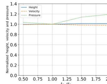
3.2.3 Ratio between stiffness parameters (pk1/k2)
Figure 11.Variation in flow height, velocity and pressure for differ-ent values of the ratio between stiffness parameters (√k1/k2) when normalized by results of the simulation withφb=30◦,
√
k1/k2=
0.3,d50=75 mm andα=30◦.
the decrease in plastic deformation at the microscale, which leads to more dispersion of particles away from the center of the flowing mass. On the contrary, for the impact pressure, an increase in√k1/k2results in a considerable decrease in the value of maximum impact pressure. The difference is very small for an increase in√k1/k2from 0.3 to 0.33. However, further increase in√k1/k2 results in a systematic decrease in the maximum applied pressure, which reaches a 40 % de-crease for √k1/k2=0.45 in comparison to
√
k1/k2=0.3. This decrease could be due to a large dispersion of particles leading to a more gradual impact on the sensor.
3.2.4 Adhesive stiffness parameter (kc)
Figure 12 shows the effect of varying the adhesive stiffness parameter (kc) on the flow height, the velocity and the pres-sure. Four values ofkc/k1are tested: 0.5, 1.0, 1.50 and 2.0. Modifying the value ofkc/k1results in a change inkcsince
k1 is fixed. The observed changes in the maximum flowing height at position 2 as well as the mean front velocity be-tween positions 1 and 2 are negligible. A slight change in the pressure applied to the large sensor is observed when increas-ingkc, especially whenkcis larger thank1. The recorded im-pact pressure is found to increase 20 % when doubling the value of (kc).
3.2.5 Mean particle diameter
Four samples with different values ofd50are tested: 75, 100, 125 and 150 mm. Values of the normalized maximum flow height at position 2, mean front velocity and maximum ap-plied pressure on the large plate are shown in Fig. 13. The maximum flow height at position 2 is found to increase when moving fromd50=75 to 100 mm while a smaller increase is observed for further increase in mean diameter (simula-tions with d50=125 and 150 mm). This increase is due to the presence of larger particles in the virtual box where flow height is measured in the model perpendicular to the base of
Figure 12.Variation in flow height, velocity and pressure for dif-ferent values of the adhesive stiffness parameter (kc) when nor-malized by results of the simulation withφb=30◦,
√
k1/k2=0.3, d50=75 mm andα=30◦.
Figure 13.Variation in flow height, velocity and pressure for differ-ent values of mean particle diameter (d50) when normalized by re-sults of the simulation withφb=30◦,
√
k1/k2=0.3,d50=75 mm andα=30◦.
Figure 14.Variation in flow height, velocity and pressure for dif-ferent values of inclination angle (α) when normalized by results of the simulation withφb=30◦,
√
k1/k2=0.3,d50=75 mm and
α=30◦.
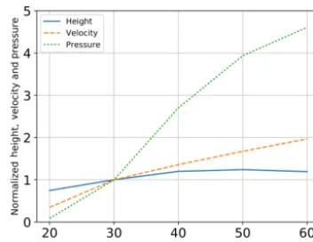
3.2.6 Inclination angle
To investigate the effect of changing the chute inclination angle (α), which was fixed at 30◦ for all other simulations in accordance with the test site in Veltheim, four additional values ofαare tested: 20, 40, 50 and 60◦. It was noted dur-ing the simulations that an inclination angle of 20◦ did not reproduce a dense flow but a very discrete flow of particles instead. This is because the value of basal frictionφbis larger thanα(GDR-MiDi, 2004). As a result, the simulation case withφb=20◦will be ignored in the results analysis.
The change in inclination angle has an effect on the maxi-mum flow height at position 2 (Fig. 10), which increases with 20 % for a change inαfrom 30 to 60◦. A larger effect is ob-served for the mean front velocity, which increases by 100 % for an increase inαto 60◦. Such an increase has a direct link to the maximum applied pressure, which increases by 465 %. All in all, the sensitivity analysis of the model’s parame-ters showed the highest sensitivity of the flow height, velocity and pressure to the variation in basal friction angle and the ratio between stiffness parameters. In the next section, dif-ferent simulations with varying values ofφband
√
k1/k2are compared to the experimental data in terms of flow height, velocity and pressure in order to find the best-fit parameter combination for each experimental test.
3.3 Cross comparison between DEM simulations and field experiments
3.3.1 Flow height and velocity
Figure 15 shows the comparison between the measured max-imum flow height at section 2 in the selected field experi-ments with values of their corresponding best-fit numerical simulations. It can be seen that a very good agreement is ob-served for tests 10 and 11 when compared with the DEM results. For tests 13–16, a relatively good agreement is
ob-Figure 15.Maximum flow height at section 2 for experimental data Exp) and their corresponding best-fit DEM simulations (H-DEM).
Figure 16.Flow front velocity, measured between sections 1 and 2, for experimental data and their corresponding best-fit DEM simula-tions.
served with the maximum margin of error being 15 %. The least agreement is shown for test no. 9, which has an error of almost+38 %. This test showed the highest variation from the mean when compared with other experimental tests.
For flowing velocity, a better general agreement between the experiment and DEM results is observed (Fig. 16). For example, for tests 10, 11 and 13, the observed mean velocity is well reproduced by the DEM. For tests 14 and 15, a rela-tively similar flow velocity of 8–9 m s−1is observed for both the experiment and the model. The only strong disagreement between the model and experiment is observed for test no. 16 for the which the experimental value is 6.4 m s−1and the cor-responding best-fit simulation flow velocity is 8.5 m s−1. 3.3.2 Impact pressure
exper-Figure 17.Maximum pressure applied to the large sensor for exper-imental data and their corresponding best-fit DEM simulations.
iment was equal to 65.9 kPa while the corresponding best-fit value recorded in the simulation was 73.8 kPa, resulting in an error of+11 %. All other tests had lower values of error when comparing pressures between the experiments and best-fit simulations. The best agreement is observed for tests 11, 15 and 16 where the errors do not exceed 4 %.
It is however important to compare the pressure evolution for the different tests, in addition to the comparison with peak pressure values. This is because the same peak pressure value could be achieved with different pressure evolution. A higher filtering interval has been applied to pressure signals of both the experiment and the DEM simulations in order to obtain pressure evolution curves that can be compared properly.
The evolution of pressure applied to the large sensor dur-ing the experimental test no. 9 is shown in Fig. 18 along with its corresponding best-fit DEM simulation. At the begin-ning of the impact (3.25< t <4.2 s), the DEM curve starts recording pressure values which are due to the dilute group of particles that are detached from the main flow and individ-ually impact the rigid wall representing the pressure sensor in the simulation. Afterwards, the two curves agree well with each other until reaching similar peak values at similar time points (64 and 70 kPa for the experiment and DEM, respec-tively). After the phase of maximum impact pressure, both pressures start decreasing with similar rates untilt=6.35 s. A further decrease in pressure is found to be faster in the ex-periment in comparison with the DEM where the decrease occurs over longer periods of time. At the end, the pressure signal in DEM is found to lag 2 s behind that of the experi-ment.
Similar observations can be made when comparing pres-sure values of test no. 14 with its corresponding DEM simu-lation (Fig. 19). A first phase of impact of the dilute group of particles causes pressure values to increase for the DEM with no equivalent increase in the experiment. Afterwards, both pressure curves agree well until reaching very similar peaks (122 and 128 kPa for the experiment and DEM, respectively). The decrease in pressure that follows the reached peaks has similar rates for both the experiment and DEM untilt=8 s.
Figure 18.Evolution of the impact pressure on the large plate for test no. 9 and its respective DEM best-fit simulation.
Figure 19.Evolution of pressure on the large plate for test no. 14 and its respective DEM best-fit simulation.
Afterwards, pressure values of the experiment decrease faster while those of DEM lag behind, causing the total impact du-ration of the DEM to be larger than that of the experiment.
Tests 11, 13 and 15, which had very similar initial con-ditions of the granular material and also similar values of measured parameters (height velocity and pressure), were found to be best fitted with similar parameter sets in YADE (φb=(25, 30, 30◦),
√
Figure 20.Evolution of pressure on the large plate for test no. 15 and its respective DEM best-fit simulation.
Figure 21.Evolution of pressure on the large plate for test no. 16 and its respective DEM best-fit simulation.
The last comparison concerns test no. 16, which is found to agree well with its corresponding best-fit DEM simulation concerning pressure evolution. Apart from the early start of the DEM curve (around 0.5 s earlier), which is due to the di-lute front, both curves are found to reach very similar peak pressure values (65 kPa for the experiment and 69 kPa for the DEM simulation) at a similar time point (t=5.2 s). Then both pressure curves start decreasing with similar rates un-tilt=7.5 s. Pressure values of test no. 16 are then found to decrease faster than those of the simulation until reaching static pressure values of around 12 kPa, which indicates the deposit of some material on the pressure sensor. The DEM curve progressively decreases over a longer period of time until decaying to zero att=12.1 s.
3.3.3 Best fit
Results of all DEM simulations are best fitted against exper-imental data of tests at the Veltheim site using Eq. (5). Fig-ure 22 shows the correspondence between experimental tests and their respective best-fit DEM parameters, based on com-parisons of flow height, flow velocity and impact pressure on the large sensor. Tests 10, 11, 13, 14 and 15 are found to be reproducible with very similar values of the param-eter set √k1/k2 andφb(Fig. 22). Those tests are found to
Figure 22.The best-fitting set of parameters (√k1/k2andφb) for each of the selected experimental tests based on comparison of flow height, mean front velocity and maximum applied pressure.
have similar values of water content in the granular material prepared in the reservoir (between 16 % and 23 %). In addi-tion, they tend to have similar values of fine content (silt and clay), which ranges between 21 % and 28 %. Test no. 9 is best reproduced by√k1/k2=0.36 andφb=25◦while test no. 16 is best reproduced by√k1/k2=0.36 andφb=40◦. Further analysis of the best-fit results and possible relations between model parameters and granular samples’ initial con-ditions are discussed in Sect. 4.2.
4 Discussion of obtained results
4.1 Phenomenology of impacting pressure
Results of the field experiments showed that the highest vary-ing parameter was the maximum impact pressure (Fig. 8). These high variations in pressure were possibly due to the interaction between large boulders of the flow and measur-ing senors in short periods of time, although this effect was minimized by filtering the data over a period of 0.05 s. This phenomenon is supported by the fact that although some tests had similar initial conditions (water and fine content) and also similar flowing height and velocity, the maximum recorded pressure was largely different. This is clear when comparing tests no. 11 and 14, which had similar values of initial and flowing conditions but different pressures of 94.6 and 138 kPa, respectively.
Figure 23. Evolution of pressure on the large plate for different simulations with differentd50, usingφb=30◦,
√
k1/k2=0.3 and
α=30◦.
which impacts the pressure sensor early (Fig. 5b). Further-more, the decreasing phase of the pressure signal was found to last longer for DEM simulations in comparison with ex-perimental tests. The formation of a dilute tail could be re-sponsible for that as it needed a longer time to fully interact with the sensor (a compression phase of the dilute part needs to first occur).
Another important factor governing the impact pressure was found to be the average particle diameter (d50). Since the total released volume is fixed, the number of particles in each simulation decreases with increasing particle size. Figure 23 shows the time evolution of pressure signal for the different tested particle size diameters. Pressure signals are found to start at relatively the same time, indicating a similar flow ar-rival time to impact the sensor. Afterwards, the peak impact pressure is reached at different time points for the different diameter sizes. Simulations with smaller particle sizes reach the peak earlier than those of larger particle sizes. However, this observation might depend on the possibility of a larger particle impacting the sensor at a specific time step. More significant is the rapid increase and decrease in the pressure signal, which is found to increase by increasing the diameter size. This could be attributed to the force chain distribution behind the wall. Force chains are strongly dependent on the particles’ position and orientation with respect to the object they impact (Azéma and Radjaï, 2012), which in this case is the large sensor. The distribution of contact forces on the sensor is expected to be different from one simulation to an-other, depending on the number of contacts and the position of large and small particles behind the sensor (Albaba et al., 2015). Figure 24 shows the maximum impact pressure and average number of contacts for different particle sizes. The use ofd50=0.075 m results in an average number of tacts for the full period of impact of 3.6. This number of con-tacts decreases rapidly with increasing average particle size reaching 1.8 contacts for d50=0.10 m and 1.4 contacts for
d50=0.15 m. Furthermore, the maximum impact pressure is found to be inversely related to the number of contacts with the sensor.
Figure 24.Maximum impact pressure and average number of con-tacts for different simulations with differentd50, usingφb=30◦,
√
k1/k2=0.3 andα=30◦.
These observations support the assumption that pressure values are mostly dominated by hard contacts with large solid grains. Such contacts influence the pressure signal, although their influence is reduced by the application of filtering win-dows. The probability of a large particle impacting the pres-sure sensor increases by increasing the mean diameter be-cause of the decrease in the number of contacts. As parti-cles grow in size and reduce in number, impact mechanisms tend to be similar to those of rockfalls (points loads) rather than those of debris flows (gradual cross-sectionally spread loads). The decrease in maximum pressure of the test with
d50=125 mm in comparison with that ofd50=100 mm can be understood through the random positioning of particles that are created in the box of the initial released volume. Par-ticles are created with random position at each simulation, which leads to different distributions of particles in the flow-ing and impactflow-ing phases.
4.2 Best-fit parameter set
DEM simulation, which is among the lowest for all best-fit simulations.
On the other hand, test no. 16 had a low water content in the released material (14 %) but a relatively high fine content (41 %). This contributed significantly to its wet density, mak-ing it the highest among all tests (2110 kg m−3). However, the low water content of the granular material might have led to its low mean front velocity, which was the lowest among all tests (6.4 m s−1). This low flowing velocity was proba-bly the main reason for the low maximum pressure value recorded during that test. All these initial conditions (espe-cially the low water content) were reflected in the value of best-fit basal friction angle parameter in the DEM simula-tion, which is highest among all best-fit simulations (40◦).
It is worth noting that attempts to base the best-fit solely on one part of Eq. (5) did not produce consistent results in terms of the relation between the initial conditions of the ex-perimental test and the model parameter set√k1/k2andφb (see Fig. A1 in Appendix A, which shows results of best-fit comparisons based separately on the flow height, the flow velocity or the impact pressure).
All in all, to draw strong conclusions on the relationship between initial conditions of granular samples and YADE model parameters, experimental data with a wider range of both water content and fine content are needed. The experi-mental data considered here had a narrow range of variation in both of those parameters, which was reflected in the nar-row variations in maximum flow height values. Since field experiments are expensive and difficult to organize, lab ex-periments can be used instead in order to study the effect of those parameters in detail.
5 Conclusions
Rapid urbanization of mountainous areas has contributed to the focus on studying the different types of mass movement such as landslides and hillslope debris flows. In this study, a discrete-element-based contact law was implemented for the purpose of modeling hillslope debris flow. The model has three phases which are elastic, plastic and adhesive. The model capabilities in reproducing filed-scale hillslope debris flow experiments were tested in detail. A group of seven ex-perimental tests were selected with varying levels of bulk density, water content and fine content. In each experiment, maximum flow height at a defined section, mean front ve-locity and maximum impact pressure applied to a measuring sensor were measured. A total of 30 numerical simulations were carried out by varying two parameters in the numerical model (basal friction angleφband the ratio between stiffness parameters√k1/k2). Calibration of the model against exper-imental data was based on finding the best-fit set of parame-tersφband
√
k1/k2of the model that matches each selected experiment concerning flow height, mean front velocity and applied pressure.
We conclude that a very good agreement between the model and experiments was observed concerning mean front velocity and maximum applied pressure, with less agreement of flow height. Detailed comparisons of pressure evolution between different selected experiments and simulations re-vealed the model’s capability of reproducing observed pres-sure curves, especially during the primary loading phase, leading to maximum pressure. However, since the model did not simulate the deposition of material on the inclined channel, a post-peak unloading phase similar to the experi-ments could not be reproduced. The analysis of the best-fit between the model and the experiments showed that many experimental tests were best reproduced with similarφband √
k1/k2 parameter combinations. These experiments were found to share similar medium values of water and fine con-tent. Increasing the basal friction in the model led to simu-lations matching the experiment with the lowest water con-tent and highest bulk density. On the contrary, a higher value of√k1/k2and relatively low value ofφbwere needed to re-produce the test with the highest water content and the lowest bulk density. All these findings suggest that a link exists be-tween the model parameters and initial conditions of granular samples. Such a link should be further investigated in detail on the basis of additional hillslope debris flow experiments.
(Fig. A1b), only on the mean front velocity (Fig. A1c) and only on the maximum applied impact pressure (Fig. A1d).
Appendix B: Results of all the selected experiments and all the simulations
The results concerning the maximum flow height at posi-tion 2, the mean front velocity and the maximum impact pressure of all selected experiments and all the simulations we carried out are shown in Table B1.
Table B1.Values of the maximum flow height at position 2, the mean front velocity and the maximum applied pressure for all selected experiments and simulations. Bold text shows the maximum values of the height, the velocity and the pressure of all selected experiments.
Exp. no./simulation Max. flow Mean front Max. pressure parameters height at velocity on large (φb−
√
k1/k2) pos. 2 (m) (m s−1) sensor (kPa)
Exp 9 0.29 10.2 65.9
Exp 10 0.40 8.2 96.0
Exp 11 0.38 9.0 94.6
Exp 13 0.33 8.4 98.5
Exp 14 0.40 9.1 138.0
Exp 15 0.37 8.9 109.4
Exp 16 0.37 6.4 69.2
Acknowledgements. The authors thank the reviewers Stéphane Lambert and Alessandro Leonardi for their constructive comments and suggestions.
Financial support. This research has been supported by the Swiss Federal Office for the Environment (FOEN).
Review statement. This paper was edited by Mario Parise and re-viewed by Alessandro Leonardi and Stéphane Lambert.
References
Albaba, A.: Discrete element modeling of the impact of granular de-bris flows on rigid and flexible structures, PhD thesis, Université Grenoble Alpes, Grenoble 2015.
Albaba, A., Lambert, S., Nicot, F., and Chareyre, B.: Relation be-tween microstructure and loading applied by a granular flow to a rigid wall using DEM modeling, Granular Matter, 17, 603–616, https://doi.org/10.1007/s10035-015-0579-8, 2015.
Albaba, A., Lambert, S., Kneib, F., Chareyre, B., and Nicot, F.: DEM Modeling of a Flexible Barrier Impacted by a Dry Granular Flow, Rock Mech. Rock Eng., 50, 3029–3048, https://doi.org/10.1007/s00603-017-1286-z, 2017.
Albaba, A., Lambert, S., and Faug, T.: Dry granular avalanche impact force on a rigid wall: Analytic shock solution ver-sus discrete element simulations, Phys. Rev. E, 97, 052903, https://doi.org/10.1103/PhysRevE.97.052903, 2018.
Andres, N. and Badoux, A.: Unwetterschäden in der Schweiz im Jahre 2017, Wasser Energie Luft, 110, 67–74, 2018.
Azéma, E. and Radjaï, F.: Force chains and contact network topol-ogy in sheared packings of elongated particles, Phys. Rev. E, 85, 31303, https://doi.org/10.1103/PhysRevE.85.031303, 2012. Brighenti, R., Segalini, A., and Ferrero, A. M.: Debris flow
hazard mitigation: A simplified analytical model for the design of flexible barriers, Comput. Geotech., 54, 1–15, https://doi.org/10.1016/j.compgeo.2013.05.010, 2013.
Bugnion, L., McArdell, B. W., Bartelt, P., and Wendeler, C.: Mea-surements of hillslope debris flow impact pressure on obsta-cles, Landslides, 9, 179–187, https://doi.org/10.1007/s10346-011-0294-4, 2012.
Catalano, E., Chareyre, B., and Barthélémy, E.: Pore-scale mod-eling of fluid-particles interaction and emerging poromechani-cal effects, Int. J. Numer. Anal. Meth. Geomech., 38, 51–71, https://doi.org/10.1002/nag.2198, 2014.
Chanut, B., Faug, T., and Naaim, M.: Time-varying force from dense granular avalanches on a wall, Phys. Rev. E, 82, 41302, https://doi.org/10.1103/PhysRevE.82.041302, 2010.
Ding, W.-T. and Xu, W.-J.: Study on the multiphase fluid-solid interaction in granular materials based on an LBM-DEM coupled method, Powder Technol., 335, 301–314, https://doi.org/10.1016/J.POWTEC.2018.05.006, 2018. Faug, T.: Depth-averaged analytic solutions for free-surface
granu-lar flows impacting rigid walls down inclines, Phys. Rev. E, 92, 62310, https://doi.org/10.1103/PhysRevE.92.062310, 2015. Faug, T., Beguin, R., and Chanut, B.: Mean steady
granular force on a wall overflowed by free-surface gravity-driven dense flows, Phys. Rev. E, 80, 021305, https://doi.org/10.1103/PhysRevE.80.021305, 2009.
Gabet, E. J. and Mudd, S. M.: The mobilization of debris flows from shallow landslides, Geomorphology, 74, 207–218, https://doi.org/10.1016/j.geomorph.2005.08.013, 2006. GDR-MiDi: On dense granular flows, Eur. Phys. J., 14, 341–365,
2004.
Graf, C. and McArdell, B. W.: Debris-flow monitoring and debris-flow runout modelling before and after construction of mit-igation measures: an example from an instable zone in the Southern Swiss Alps, in: La géomorphologie alpine: entre pat-rimoine et contrainte. Actes du colloque de la Société Su-isse de Géomorphologie, 3–5 septembre 2009, Olivone (Géo-visions no. 36). Institut de géographie, Université de Lausanne, edited by: Lambiel, C., Reynard, E.. and Scapozza, C., p. 11, available at: https://www.unil.ch/files/live/sites/igd/files/shared/ Geovisions/Geovisions36/16_Graf_McArdell.pdf (last access: 1 August 2019), 2011.
Horton, P., Jaboyedoff, M., Rudaz, B., and Zimmermann, M.: Flow-R, a model for susceptibility mapping of debris flows and other gravitational hazards at a regional scale, Nat. Hazards Earth Syst. Sci, 13, 869–885, https://doi.org/10.5194/nhess-13-869-2013, 2013.
Hungr, O.: A model for the runout analysis of rapid flow slides, de-bris flows, and avalanches, Can. Geotech. J., 32, 610–623, 1995. Hungr, O., Leroueil, S., and Picarelli, L.: The Varnes classifica-tion of landslide types, an update, Landslides, 11, 167–194, https://doi.org/10.1007/s10346-013-0436-y, 2014.
Hürlimann, M., McArdell, B. W., and Rickli, C.: Field and laboratory analysis of the runout characteristics of hillslope debris flows in Switzerland, Geomorphology, 232, 20–32, https://doi.org/10.1016/j.geomorph.2014.11.030, 2015. Iverson, R. M. and LaHusen, R. G.: Friction in debris flows:
In-ferences from large-scale flume experiments, Hydraul. Eng., 93, 1604–1609, 1993.
Iverson, R. M., Reid, M. E., and LaHusen, R. G.: Debris-Flow Mo-bilization From Landslides, Annu. Rev. Earth Planet. Sci., 25, 85–138, https://doi.org/10.1146/annurev.earth.25.1.85, 1997. Jiang, Y. J. and Towhata, I.: Experimental study of dry granular
Jibson, E. L. H. R. W.: Inventory of landslides triggered by the 1994 Northridge, California earthquake, USGS Midwest Area, Reston, VA, USA, 1995.
Kattel, P., Kafle, J., Fischer, J. T., Mergili, M., Tuladhar, B. M., and Pudasaini, S. P.: Interaction of two-phase debris flow with obstacles, Eng. Geol., 242, 197–217, 2018.
Klubertanz, G., Laloui, L., and Vulliet, L.: Identification of mech-anisms for landslide type initiation of debris flows, Eng. Geol., 109, 114–123, https://doi.org/10.1016/j.enggeo.2009.06.007, 2009.
Kneib, F., Faug, T., Nicolet, G., Eckert, N., Naaim, M., and Dufour, F.: Force fluctuations on a wall in interaction with a granular lid-driven cavity flow, Phys. Rev. E, 96, 042906, https://doi.org/10.1103/PhysRevE.96.042906, 2017.
Kneib, F., Faug, T., Dufour, F., and Naaim, M.: Mean force and fluctuations on a wall immersed in a sheared granular flow, Phys. Rev. E, 99, 052901, https://doi.org/10.1103/PhysRevE.99.052901, 2019.
Leonardi, A., Wittel, F. K., Mendoza, M., Vetter, R., and Herrmann, H. J.: Particle-Fluid-Structure Interaction for Debris Flow Im-pact on Flexible Barriers, Comput.-Aid. Civ. Infrastruct. Eng., 31, 323–333, https://doi.org/10.1111/mice.12165, 2016. Luding, S.: Cohesive, frictional powders: contact models for
ten-sion, Granular Matter, 10, 235–246, 2008.
Maurin, R., Chauchat, J., and Frey, P.: Dense granular flow rheol-ogy in turbulent bedload transport, J. Fluid Mech., 804, 490–512, 2016.
Mede, T., Chambon, G., Hagenmuller, P., and Nicot, F.: A medial axis based method for irregular grain shape rep-resentation in DEM simulations, Granular Matter, 20, 16, https://doi.org/10.1007/s10035-017-0785-7, 2018.
Montrasio, L. and Valentino, R.: Modelling rainfall-induced shal-low landslides at different scales using SLIP – Part I, Proced. Eng., 158, 476–481, 2016.
Olivares, L. and Picarelli, L.: Shallow flowslides triggered by intense rainfalls on natural slopes covered by loose unsaturated pyroclastic soils, Géotechnique, 53, 283–287, https://doi.org/10.1680/geot.2003.53.2.283, 2003.
Papachristos, E., Scholtès, L., Donzé, F., and Chareyre, B.: Intensity and volumetric characterizations of hydraulically driven frac-tures by hydro-mechanical simulations, Int. J. Rock Mech. Min. Sci., 93, 163–178, 2017.
Ran, Q., Hong, Y., Li, W., and Gao, J.: A modelling study of rainfall-induced shallow landslide mechanisms under different rainfall characteristics, J. Hydrol., 563, 790–801, 2018. Scherer, B.: MFLOW – Ein Modell zur Simulation von
Hang-muren, BSc thesis, Tech. rep., Bern University of Applied sci-ences, Bern, 2016.
Schwager, T. and Poeschel, T.: Coefficient of restitution and linear dashpot model revisited, Granular Matter, 9, 465–469, https://doi.org/10.1007/s10035-007-0065-z, 2007.
Schwarz, M., Lehmann, P., and Or, D.: Quantifying lateral root reinforcement in steep slopes – from a bundle of roots to tree stands, Earth Surf. Proc. Land., 35, 354–367, https://doi.org/10.1002/esp.1927, 2010.
Shen, P., Zhang, L., Chen, H., and Gao, L.: Role of vegetation restoration in mitigating hillslope ero-sion and debris flows, Eng. Geol., 216, 122–133, https://doi.org/10.1016/J.ENGGEO.2016.11.019, 2017. Shen, W., Zhao, T., Zhao, J., Dai, F., and Zhou, G. G.:
Quantifying the impact of dry debris flow against a rigid barrier by DEM analyses, Eng. Geol., 241, 86–96, https://doi.org/10.1016/J.ENGGEO.2018.05.011, 2018. Silbert, L. E., Erta’cs, D., Grest, G. S., Halsey, T. C., Levine, D.,
Plimpton, S. J., Ertas, D., Grest, G. S., Halsey, T. C., Levine, D., and Plimpton, S. J.: Granular flow down an inclinedrheol-ogy Bagnold scaling and Rheolinclinedrheol-ogy, Phys. Rev. E, 64, 51302, https://doi.org/10.1103/PhysRevE.64.051302, 2001.
Šmilauer, V., Catalano, E., and Chareyre, B.: Yade documentation, . . . Yade Project, https://doi.org/10.5281/zenodo.34073, 2010. Teufelsbauer, H., Wang, Y., Chiou, M. C., and Wu, W.:
Flow-obstacle interaction in rapid granular avalanches: DEM simula-tion and comparison with experiment, Granular Matter, 11, 209– 220, https://doi.org/10.1007/s10035-009-0142-6, 2009. Teufelsbauer, H., Wang, Y., Pudasaini, S. P., Borja, R. I., and
Wu, W.: DEM simulation of impact force exerted by gran-ular flow on rigid structures, Acta Geotech., 6, 119–133, https://doi.org/10.1007/s11440-011-0140-9, 2011.
Voellmy, A.: Über die Zerstorungskraft von Lawinen, Schweiz-erische Bauzeitung, 73, 159–162, 1955.
Volkwein, A.: Numerical simulation of flexible rockfall protec-tion systems. in: Proceedings of the internaprotec-tional conference on Computing in Civil Engineering, edited by: Soibelman, L. and Feniosky, P. M., 11 pp., https://doi.org/10.1061/40794(179)122, 2005.
Vollmöller, P.: A shock-capturing wave-propagation method for dry and saturated granular flows, J. Comput. Phys., 199, 150–174, https://doi.org/10.1016/J.JCP.2004.02.008, 2004.
Šmilauer, V., et al.: Using and Programming, in: Yade Documentation, 2nd Edn., The Yade Project, https://doi.org/10.5281/zenodo.34043, 2015.