IJEDR1503021 International Journal of Engineering Development and Research (www.ijedr.org) 1
Behaviour of Multilayer Feed Forward Networks on
Multidisciplinary Data
1Syed Aamiruddin
1 Assistant Professor, University School Of Communication and Technology, Guru Govind Singh Indraprastha University , Dwarka ,New Delhi
________________________________________________________________________________________________________
Abstract - The fact that the signature is widely used as a means of personal verification emphasizes the need for an automatic verification system. Verification can be performed either Offline or Online based on the application. Online systems use dynamic information of a signature captured at the time the signature is made. Offline -signatures using a set of simple shape based geometric features. And applied Multilayer feed forward networks on multidisciplinary data including signatures for results.
Keywords - Artificial Neural Networks. Hidden layers, Generalized Delta rule, Offline Signature Verification
______________________________________________________________________________________
I. INTRODUCTION
The work on artificial neural network [4] has been motivated right from its inception by the recognition that the human brain computes in an entirely different way from the conventional digital computer. The brain is a highly complex, nonlinear and parallel information processing system. It has the capability to organize its structural constituents, known as neurons, so as to perform certain computations many times faster than the fastest digital computer in existence today. The brain routinely accomplishes perceptual recognition tasks, e.g. recognizing a familiar face embedded in an unfamiliar scene, in approximately 100-200 ms, whereas tasks of much lesser complexity may take days on a conventional computer. A neural network is a machine that is designed to model the way in which the brain performs a particular task. The network is implemented by using electronic components or is simulated in software on a digital computer. A neural network is a massively parallel distributed processor made up of simple processing units, which has a natural propensity for storing experimental knowledge and making it available for use. Artificial neural networks (ANNs) provide a new suite of nonlinear algorithms for feature extraction using hidden layers and classification. In addition, existing feature extraction and classification algorithms can also be mapped on neural network architectures for efficient implementation. It resembles the brain in two respects:
1. Knowledge is acquired by the network from its environment through a learning process.
2. Interneuron connection strengths, known as synaptic weights, are used to store the acquired knowledge.
Neural networks, with their remarkable ability to derive meaning from complicated or imprecise data, can be used to extract patterns and detect trends that are too complex to be noticed by either humans or other computer techniques. Other advantages include:
1. Adaptive learning: An ability to learn how to do tasks based on the data given for training or initial experience.
2. Self-Organization: An ANN can create its own organization or representation of the information it receives during learning time.
3. Real Time Operation: ANN computations may be carried out in parallel, and special hardware devices are being designed and manufactured which take advantage of this capability.
Neural networks have broad applicability to real world business problems and have already been successfully applied in many industries. Since neural networks are best at identifying patterns or trends in data, they are well suited for prediction or forecasting needs including:
‒ Sales forecasting ‒ Industrial process control ‒ Customer research ‒ Data validation ‒ Risk management ‒ Target marketing etc.
II.METHODOLOGY
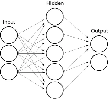
IJEDR1503021 International Journal of Engineering Development and Research (www.ijedr.org) 2 Fig 2.1: Multi-layer Feed-forward Network
For determination of number of hidden units in ANN, we have some traditional approach to follow:
a) Try different configurations, see what works best. We can divide our training set into two pieces one for training, one for evaluation and then train and evaluate different approaches. Unfortunately it sounds like in our case this experimental approach isn't available.
b) Use a rule of thumb. Concerning the number of neurons in the hidden layer, it has been speculated that (for example) it should: (i) be between the input and output layer size,
(ii) set to something near (inputs + outputs) * 2/3, or (iii) never larger than twice the size of the input layer.
A.Multi-layer Perceptron
Multi-Layer perceptron (MLP) is a forward neural network with one or more layers between input and output layer. A feed-forward network has a layered structure as shown in fig 2.4. Each layer consists of units which receive their input from units from a layer directly below and send their output to units in a layer directly above the unit. There are no connections within a layer. The Ni inputs are fed into the first layer of Nh,1 hidden units. The input units are merely 'fan-out' units; no processing takes place in these units. The activation of a hidden unit is a function Fi of the weighted inputs plus a bias. The output of the hidden units is distributed over the next layer of Nh,2 hidden units, until the last layer of hidden units, of which the outputs are fed into a layer of No output units. We have adopted this approach with backpropagation as explained in following sections.
A single-layer network has severe restrictions: the class of tasks that can be accomplished is very limited. Minsky and Papert showed in 1969 that a two layer feed-forward network can overcome many restrictions, but did not present a solution to the problem of how to adjust the weights from input t-o hidden units. An answer to this question was presented by Rumelhart, Hinton and Williams in 1986 and similar solutions appeared to have been published earlier. The central idea behind this solution is that the errors for the units of the hidden layer are determined by back-propagating the errors of the units of the output layer. For this reason the method is often called the back-propagation learning rule. Back-propagation can also be considered as a generalization of the delta rule for non-linear activation functions and multilayer networks.The backpropagation learning algorithm which is adopted in our work can be divided into two phases: propagation and weight update.
Phase 1: Propagation
Each propagation involves the following steps:
1. Forward propagation of a training pattern's input through the neural network in order to generate the propagation's output activations.
2. Backward propagation of the propagation's output activations through the neural network using the training pattern target in order to generate the deltas of all output and hidden neurons.
Phase 2: Weight Update
For each weight-synapse follow the following steps:
1. Multiply its output delta and input activation to get the gradient of the weight.
2. Bring the weight in the opposite direction of the gradient by subtracting a ratio of it from the weight.
This ratio influences the speed and quality of learning; it is called the learning rate. The sign of the gradient of a weight indicates where the error is increasing; this is why the weight must be updated in the opposite direction. Repeat phase 1 and 2 until the performance of the network is satisfactory.We worked with the three layer network, an algorithm of which follows:
1. Initialize the weights in the network (often small random values) do2. for each pattern p in the training set
3. O = neural-net-output (network, p) // forward pass 4. T = teacher output for p
5. Compute error (T - O) at the output units
IJEDR1503021 International Journal of Engineering Development and Research (www.ijedr.org) 3
𝑠𝑘 (𝑡) = ∑ 𝑤𝑗 𝑗𝑘 (𝑡) ∗ 𝑦𝑗(𝑡) + 𝜃𝑘(𝑡)) (2.1)
7. Compute delta_wi for all weights from input layer to hidden layer // backward pass continued
𝑠𝑗 (𝑡) = ∑ 𝑤𝑖 𝑖𝑗 (𝑡) ∗ 𝑦𝑖(𝑡) + 𝜃𝑗(𝑡)) (2) 8. update the weights in the network.
9. until all examples classified correctly or stopping criterion satisfied 10. return the network
Backpropagation calculates the gradient of the error of the network regarding the network's modifiable weights. This gradient is almost always used in a simple stochastic gradient descent algorithm to find weights that minimize the error. Often the term "back-propagation" is used to refer to the entire procedure comprising of both the calculation of the gradient and its use in stochastic gradient descent . Back-propagation usually allows quick convergence on satisfactory local minima for error in the kind of networks to which it is suited.
Backpropagation networks are necessarily multilayer perceptron (usually with one input, one hidden, and one output layer). In order for the hidden layer to serve any useful function, multilayer networks must have non-linear activation functions for the multiple layers: a multilayer network using only linear activation functions is equivalent to some single layer, linear network.
B. The Generalized Delta rule
The application of the generalized delta rule thus involves two phases: During the first phase the input x is presented and propagated forward through the network to compute the output values 𝑦0𝑝for each output unit. This output is compared with its desired value 𝑑𝑜, resulting in an error signal 𝛿0 𝑝for each output unit. The second phase involves a backward pass through the network during which the error signal is passed to each unit in the network and appropriate weight changes are calculated.
Weight adjustments with sigmoid activation function
The results from the previous section can be summarized in following equations:
The weight of a connection is adjusted by an amount proportional to the product of an error signal δ, on the unit k receiving the input and the output of the unit j sending this signal along the connection:
∆𝑝𝑤𝑗𝑘 = 𝛾𝛿𝑘 𝑝𝑦𝑗𝑝 (3)
If the unit is an output unit, the error signal is given by 𝛿0 𝑝= 𝑑0𝑝− 𝑦0𝑝𝑓′(𝑠
0
𝑝) (4)
Take as the activation function F the 'sigmoid' function as,
𝑦𝑝= 𝑓(𝑠𝑝) = 1
1+𝑒−𝑠𝑝 (5)
In this case ,the derivative of eqn 5 is equal to: 𝑓′(𝑠 0 𝑝 ) = 𝛿 𝛿𝑠𝑝 1 1+𝑒−𝑠𝑝 = 1
1+𝑒−𝑠𝑝(−𝑒−𝑠 𝑝 ) = 1 1+𝑒−𝑠𝑝 (−𝑒−𝑠𝑝 1+𝑒−𝑠𝑝
=𝑦𝑝(1 − 𝑦𝑝) (6)
Such that the error signal for an output unit using eqn.6 in eqn 4 can be written as: 𝛿0 𝑝= (𝑑0𝑝− 𝑦0𝑝)𝑦0𝑝(1 − 𝑦𝑝) (7)
The error signal for a hidden unit is determined recursively in terms of error signals of the units to which it directly connects and the weights of those connections. For the sigmoid activation function:
𝛿ℎ 𝑝 = 𝑓′(𝑠 ℎ 𝑝) ∑ 𝛿 0 𝑝𝑤 ℎ𝑜 𝑁0
𝑜=1 = 𝑦ℎ
𝑝(1 − 𝑦 ℎ 𝑝) ∑ 𝛿 0 𝑝𝑤 ℎ𝑜 𝑁0
𝑜=1 (2.8)
We will get an update rule which is equivalent to the delta rule as described in the previous chapter, resulting in a gradient descent on the error surface if we make the weight changes according to:
∆𝑝𝑤𝑗𝑘 = 𝛾𝛿𝑘 𝑝𝑦𝑗𝑝 (9)
The equation (10) gives a recursive procedure for computing the δ's for all units in the network, which are then used to compute the weight changes accordingly.
𝛿ℎ 𝑝= 𝑓′(𝑠
IJEDR1503021 International Journal of Engineering Development and Research (www.ijedr.org) 4 This procedure constitutes the generalized delta rule for a feed-forward network of non-linear units. The whole back-propagation process is intuitively very clear. What happens in the above equations is the following. When a learning pattern is clamped, the activation values are propagated to the output units, and the actual network output is compared with the desired output values, we usually end up with an error in each of the output units. The simplest method to do this is the greedy method: we strive to change the connections in the neural network in such a way that, next time around, the error eo will be zero for this particular pattern. That's step one. But it alone is not enough: when we only apply this rule, the weights from input to hidden units are never changed, and we do not have the full representational power of the feed-forward network as promised by the universal approximation theorem. In order to adapt the weights from input to hidden units, we again want to apply the delta rule. In this case, however, we do not have a value for δ for the hidden units. This is solved by the chain rule which does the following: distribute the error of an output unit o to all the hidden units that is it connected to, weighted by this connection. Differently put, a hidden unit h receives a delta from each output unit o equal to the delta of that output unit weighted with (= multiplied by) the weight of the connection between those units.
Although back-propagation can be applied to networks with any number of layers, just as for networks with binary units it has been shown that only one layer of hidden units suffices to approximate any function with finitely many discontinuities to arbitrary precision, provided the activation functions of the hidden units are non-linear. In most applications a feed-forward network with a single layer of hidden units is used with a sigmoid activation function for the units.
Dataset Obtained
We are also dealing with verification of Offline Signature images. The following is steps of obtaining signature data set:
i) Image acquisition: Image is obtained by scanning handwritten human signatures. We have obtained a set of five signatures for 68 persons. The pre-processing of the images is discussed in following sections.
ii) Converting Color image to gray scale image: In the system, all image capturing and scanning devices use colour. Therefore, we also used a Color scanning device to scan signature images. A colour image consists of a coordinate matrix and three colour matrices. Coordinate matrix contains x, y coordinate values of the image. The colour matrices are labelled as red (R), green (G), and blue (B). Techniques presented in this study are based on grey scale images, and therefore, scanned colour images are initially converted to grey scale as shown in example:
Gray colour = 0.299*Red + 0.5999*Green +0.111*Blue
iii) Noise Reduction: Noise reduction is one of the most important processes in image processing. Images are often corrupted due to positive and negative impulses stemming from decoding errors or noisy channels. An image may also be degraded because of the undesirable effects due to illumination and other objects in the environment. We have used thinning for reducing the noise. Thinning is a operation that is used to remove selected foreground pixels from binary images.
iv)Background elimination and border clearing: Our applications require the differentiation of objects from the image background. Clustering based thresholding is choosing a threshold value T and assigning 0 to the pixels with values smaller than or equal to T and 1 to those with values greater than T.
v) Signature normalization: Signature dimensions may vary due to the irregularities in the image scanning and capturing process. Furthermore, height and width of signatures vary from person to person and, sometimes, even the same person may use different size signatures. First, we need to eliminate the size differences and obtain a standard signature size for all signatures. After this normalization process, all signatures will have the same dimensions.
vi)Feature Extraction: Transforming the input data into the set of features is called feature extraction. Feature Extraction is the key to develop an offline signature recognition system. These features are geometrical features based on the shape and dimensions of a signature image.In this data set we need to classify signature according to the no of person. For each person a set of five signatures is maintained over a period of time. The ten features extracted for this problem is also called global features [3].They are as follows:
Edge Point: The edge point is a point that has only one of 8×8 neighbour. In order to extract the edge points in a given signature, we used a 3×3 structuring element with all coefficients equal to 1.
Cross Point: Cross point is a point that has at least three of 8×8 neighbours. The structuring element that was used to extract edge points, was also used to extract the cross points in a signature. Number of cross points is a nice feature to distinguish signatures.
Closed Loops: The number of closed loop in the image.
Signature Height: It is the maximum row size of the image.
Pure Width: The actual width of the image, it is given by number of row while traversing in row major order.
Vertical Center: The center of image while traversing in column major order.
Horizontal Center: The center of image while traversing in row major order.
Maximum Vertical Projection: Sum of points in each row of an image is called the vertical projection. 𝑣(𝑖) = ∑ 𝐼(𝑖, 𝑗)𝑛𝑖 (1)
Maximum Horizontal Projection: Sum of points in each column of an image is called the Horizontal projection. ℎ(𝑖) = ∑ 𝐼(𝑖, 𝑗)𝑛𝑗 (2)
Image Area: The total number of points is called Image area. Here these points will be black pixel.
III.RESULT
IJEDR1503021 International Journal of Engineering Development and Research (www.ijedr.org) 5 Table I Table of Data Set description
Data set Data set Name No. of Tuples No. of attributes No. of Classes
I Nursery 12961 9 5
II Car Evaluation 1728 7 4
III Zoo 101 16 7
IV Signature 340 10 68
V Tic Tac Toe 958 9 2
The performance of a classifier is measures in term of its accuracy, speed, robustness, scalability and its interpretability. Out of all these we have chosen to evaluate the classifier performance with respect to accuracy and speed only.
To measure robustness, we need extensive data pre-processing techniques, which may well be our future focus. To estimate scalability, we tested our algorithm with a large dataset containing 12961 tuples and 9 attributes.
We have performed experiment on all data set, by considering generalisation with respect to test accuracy. We have taken the ratio of training ,generalisation and test set as 60, 20 and 20 respectively. Here generalisation accuracy is used for checking whether to proceed to back-propagation. The following figure 4.1, the result is shown.
Table II: Result shown for accuracy (%) over different data sets with learning rate set at 0.3 Accuracy
Table
Tic-Tac-Toe Zoo Car Nursery Signature
Training Set 88.15 100 88.7 97 95.22
Generalization Set 79.16 100 88.72 96.52 66.76
Testing Set 79.16 80 87.28 97.49 84.55
We can depict that as for all dataset except signature generalisation accuracy is greater than training accuracy so overfiting is under control.For signature dataset, the generalisation and training error meet after a epoch of 800 at 0.01446,but generalisation accuracy is still low but there is less overfitting as we are still getting a good test accuracy.
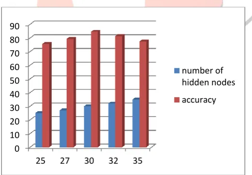
In the following fig 1, we have conducted set of experiments on signature images and it reflects performance of ANN with respect to different number of hidden nodes.
For performance tuning, we need to try for different number of hidden node but here we have considered arithmetic mean for the base, then gradually increasing we got different results.
Fig 1: Variation of accuracy with the number of hidden nodes. IV.CONCLUSION & FUTURE SCOPES
The artificial neural network has established itself as a fruitful approach for developing an intelligent information processing system. In particular, ANNs have been viewed as a powerful tool in modern AI techniques. From the above results it is obvious that the performance of ANN model improves in case of large data sets such as nursery data set as well as in case of complex domain data such as signature images. In case of complex domain data, the most crucial phase is feature extraction. The more the variety of features, the better will be the result. As we have only considered geometric features, other type of feature can also be considered like angular features. We will be also looking in feasibility of taking Online Signature data set into account that will add more dimensions to the neural network and comparing those results with the present. Other future areas of work may be to verify different data sets using other techniques like Support Vector Machines and Radial Basis Function networks. As mentioned earlier, the input features of the signature data set can also be changed. So, the future work of the verification of signature can be done with the same Neural Network methods but using different signature features and compares the results with those obtained in the present work. We will also be exploring ANN-based approaches towards designing CBR system.
0 10 20 30 40 50 60 70 80 90
25 27 30 32 35
number of hidden nodes
IJEDR1503021 International Journal of Engineering Development and Research (www.ijedr.org) 6 REFERENCE
[1] Han J. ,Kamber M., “Data Mining Concepts and Techniques,” Morgan Kaufmann Publishers, San Francisco, USA, 2001, ISBN 1558604898
[2] Aleksander, I., Morton H., 1995. An Introduction to Neural Computing (2nd ed). Chapman and Hall
[3] McCabe,A., Trevathan, J., Wayne,R., “Neural Network-based Handwritten Signature Verification”, Journal of Computers ,Vol.3, No .8,August 2008.
[4] Bajaj R., Chaudhary S., "Signature Verification using multiple neural classifiers”, Pattern recognition society 30,(1996),1-7 [5] http://archive.ics.uci.edu/ml/machine-learning-databases
[6]Ostu N., 'A Threshold Selection Method from Gray Level Histogram', IEEE Trans. on Systems, Man and Cybernetics, SMC-8, 1978, pp. 62-66.
[7] Qi.Y, Hunt B.R., 'Signature Verification using Global and Grid Features', Pattern Recognition, Vol. 27, No. 12, 1994, pp. 1621-1629