Mean-field type games between two players driven by backward stochastic differential equations

Mean-field type games between two players driven

by backward stochastic differential equations

Alexander Aurell †

September 3, 2018

Abstract: In this paper, mean-field type games between two players with backward stochastic dynamics are defined and studied. They make up a class of non-zero-sum dif-ferential games where the players’ state dynamics solve backward stochastic difdif-ferential equations (BSDEs) that depend on the marginal distributions of player states. Players try to minimize their individual cost functionals, also depending on the marginal state distri-butions. Under some regularity conditions, we derive necessary and sufficient conditions for existence of Nash equilibria. Player behavior is illustrated by numerical examples, and is compared to a centrally planned solution where the social cost, the sum of player costs, is minimized. The inefficiency of a Nash equilibrium, compared to socially optimal be-havior, is quantified by the so-called price of anarchy. Numerical simulations of the price of anarchy indicate how the improvement in social cost achievable by a central planner depends on problem parameters.

MSC 2010: 49N10, 49N70, 49N90, 91A13, 93E20

Keywords: Mean-field type game, Non-zero-sum differential game, Coopera-tive game, Backward stochastic differential equations, Linear-quadratic stochas-tic control, Social cost, Price of anarchy

1. Introduction

A mean-field type game (MFTG) is a game in which payoffs and dynamics depend not only on the state and control profiles of the players, but also on the distribution of the state-control processes. MFTG has a plethora of applications in the engineering sciences, see [15] and the references therein.

The theory of MFTG and mean-field type control (MFTC), initiated in [1], is well developed for forward stochastic dynamics, i.e. given initial conditions [5, 8, 12]. In the deterministic case, initial and terminal conditions are equivalent. However, in the stochastic case they are not, and there are applications where stochastic dynamics with terminal conditions are of interest; in [3], we propose a model for pedestrians groups moving towardstargets they must reach, such as deliveries and emergency personnel. The hard terminal condition leads to the formulation of a dynamic model for crowd motion where the state dynamics satisfies a BSDE. A game between such groups is of interest since it could be a tool for decentralized decision making

∗

Financial support from the Swedish Research Council (2016-04086) is gratefully acknowledged. The author would like to thank B. Djehiche for fruitful discussions and useful suggestions regarding this manuscript.

†

Department of Mathematics, KTH Royal Institute of Technology, 100 44 Stockholm, Sweden. E-mail address: [email protected]

1

under conflicting interests. Mean-field effects appear in pedestrian crowd models as approxima-tions of aggregate human interaction, so the game would in fact be a MFTG [2]. Other areas of application include strategies for financial investments, where often future conditions are specified [14, 17, 18, 19, 21] and lead to dynamic models using BSDEs. On financial markets, price is determined by the aggregates (mean-field effects) such as supply and demand, and players on that market naturally compete.

BSDEs were introduced in [6] and the general theory is by now fully developed [28, 31]. Optimal control of BSDEs with coefficients involving the marginal state distribution, mean-field BSDEs, has recently gained attention. A key tool in optimal control of BSDEs (and SDEs) is the anal-ysis of forward-backward systems of stochastic differential equations, arising both in dynamic programming and from the Pontryagin type stochastic maximum principle. Forward-backward SDEs are thoroughly treated in [30, 31], and the mean-field version in [12]. Mean-field BSDEs were derived as limits of particle systems in [7]. Existence and uniqueness results for mean-field BSDEs, as well as a comparison theorem, are provided in [9]. In [25] the linear-quadratic BSDE control problem with deterministic coefficients is studied. Recent work on the control of BSDEs includes [24, 29].

The natural next step is to extend control of mean-field BSDEs to games where the state pro-cesses are mean-field BSDEs. In this paper we analyze a game between two players following mean-field BSDE dynamics. This is in fact a MFTG, since the distribution of each player is effected by both players’ choice of strategy. We also look at the cooperative situation, which is a control problem, where a central planner optimizes the social cost. The social cost is the the sum of player costs. The fraction between the worst case social cost in the game and the optimal social cost quantifies the efficiency of game equilibria and was first studied in [22] for traffic coordination on networks under the namecoordination ratio. Later, [26] coined the term price of anarchy.

Following the path laid-out in [1], we derive necessary and sufficient conditions for equilibria and social optima, establishing a Pontryagin type maximum principle under Lipschitz and differentiability assumptions on the involved cost and dynamic coefficient functions. As a con-sequence, we have existence of a Nash equilibrium and a verification theorem. We solve a linear-quadratic (LQ) case explicitly up to a system of ordinary differential equations (ODEs) and provide numerical examples that pinpoint differences in player behavior between the game and the centrally planned case. We study the price of anarchy, the price the players as a society have to pay for having independent choice, by simulation in the LQ case. By varying parame-ters, we observe how a central planner’s improvement depends on the players’ preferences.

2. Problem formulation

LetT >0 be a finite real number representing the time horizon of the game. Consider a filtered probability space (Ω,F,{F_t}_t≥0,P) on which two independent standard Brownian motions

W·1, W·2 are defined, d1- and d2-dimensional respectively. Additionally, yT1, yT2 ∈ L2FT(Ω;R

d₎

and ξ, F0-measurable, are defined on the space. We assume that these five random objects are independent and that they generate the filtration F := {Ft}t≥0. Notice that ξ makes F0 non-trivial. LetGbe theσ-algebra on [0, T]×Ω ofFt-progressively measurable sets. Fork≥1,

let S2,k be the set of Rk-valued and continuous G-measurable processes X·:={Xt:t∈[0, T]}

such thatE[supt∈[0,T]|Xt|2]<∞, and letH2,k be the set ofRk-valued G-measurable processes

X·such that E[R₀T |Xs|2ds]<∞.

Let (Ui, d_Ui) be a separable metric space, i= 1,2. Player ipicks her controlui_· from the set

Ui:=

u : [0, T]×Ω→Ui |u· is F-adapted, E

Z T

0

d_Ui(us)2ds

<∞

. (2.1)

The distribution of any random variable χ∈ X will be denoted by L(ξ)∈ P(X), and −iwill denote the index {1,2}\i. Given a pair of controls (u·1, u2·) ∈ U1× U2, consider the system of

controlled BSDEs

dY_ti=bi(t,Θi_t,Θ−_ti, Zt)dt+Z_ti,1dW_t1+Z_ti,2dW_t2, Y_Ti =y_Ti, i= 1,2, (2.2) where Θi_t= (Y_ti,L(Y_ti), ui_t) and Zt= [Z_t1,1Z_t1,2Z_t2,1Z_t2,2]. Furthermore,

bi: Ω×[0, T]×S×Ui×S×U−i×Rd×(2d1+2d2)→Rd, (2.3)

where S := Rd× P(Rd) is equipped with the norm k(y, µ)kS := |y|+d2(µ), d2 being the 2-Wasserstein metric onP(Rd).Rd×(2d1+2d2)is equipped with the trace normkZkF = tr(ZZ∗)1/2.

Note that if X is a square integrable random variable in Rd, then d2(L(X)) < ∞ and L(X)∈ P₂(Rd), the space of measures with finited2-norm.

Given (u1·, u2·)∈ U1×U2, a pair ofRd×Rd×(d1+d2)-valuedG-measurable processes (Y·i,[Z·i,1Z·i,2]),

i= 1,2, is a solution to (2.2) if

Y_ti =y_Ti −

Z T

t

bi(s,Θi_s,Θ−_si, Zs)ds−

2

X

j=1

Z T

t

Z_si,jdW_sj, ∀t∈[0, T], a.s., (2.4)

and (Y·i,[Z·i,1Z·i,2])∈S2,d×H2,d×(d1+d2).

Remark 2.1. Any terminal condition yi_T ∈ L2_F

T(Ω;R

d_{) naturally induces a}

F-martingale

Y_ti := E[yiT | Ft]. The martingale representation theorem then gives existence of a unique

process [Z·i,1, Z·i,2]∈H2,d×(d1+d2)such thatYti =yTi +Z i,1

t dWt1+Z i,2

t dWt2, i.e. [Z i,1

· , Z·i,2] plays

the role of the projection and without it, Y_·i would not be G-measurable. Hence the noise (W1

·, W·2) generating the filtration is common to both players, and [Z

i,1

· , Z·i,2], i= 1,2 is their

it is a second control of player i: first she plays ui

· to heed preferences on energy use, initial

position etc., then she picks [Z·i,1, Z·i,2] so that her path to yi_T is the optimal prediction based

on available information in the filtration at any given time. The component bi in (2.2) acts as a velocity in.

Existence and uniqueness of (2.2) is given by a slight variation of [9, Theorem 3.1], where the one-dimensional case is treated. For the d-dimensional mean-field free case, see [27].

Assumption 1. The process bi(ω,·,0, . . . ,0), i = 1,2, belongs to H2,d and for any vi =

(yi, µi, ui, y−i, µ−i, u−i, z)∈S×U1×S×U2×Rd×(2d1+2d2),bi(ω,·, vi),i= 1,2, isG-measurable.

Assumption 2. Given a pair of control values(u1, u2)∈U1×U2, there exists a constantL >0 such that for all t∈[0, T]and tuples (y1, µ1, y2, µ2, z),(¯y1,µ¯1,y¯2,µ¯2_{,z¯)∈S×S×R}d(2d1+2d2)

|bi(t, yi, µi, ui, y−i, µ−i, u−i, z)−bi(t,y¯i,µ¯i, ui,y¯−i,µ¯−i, u−i,z¯)|

≤L 



2

X

j=1

k(yj, µj)−(¯yj,µ¯j)kS+kz−z¯kF 

, P-a.s., i= 1,2.

(2.5)

Theorem 2.1. Let Assumptions 1 and 2 hold. Then, for any terminal conditions y1_T, y2_T ∈

L2(Ω,FT,P;Rd) and (u1·, u2·)∈ U1× U2, the system of mean-field BSDEs (2.2) has a unique

solution (Y_·i,[Z·i,1, Z·i,2])∈S2,d×H2,d×(d1+d2), i= 1,2.

Next, we introduce the best reply of playeri as follows:

Ji(ui·;u−· i) :=E

Z T

0

fi(t,Θi_t,Θ_t−i)dt+hi(Y₀i,L(Y₀i), Y₀−i,L(Y₀−i))

(2.6)

for given maps fi : [0, T]×S×Ui×S×U−i →_Rand hi : Ω×S×S→_R.

Assumption 3. For any pair of controls(u1·, u2·)∈ U1× U2, fi(·,Θi·,Θ−· i)∈L1F(0, T;R) and

h(Y₀i,L(Y₀i), Y₀−i,L(Y₀−i))∈L1_F

0(Ω;R).

The problems we consider next are

1. The Mean-field Type Game (MFTG): find the Nash equilibrium controls of







inf

ui

·∈Ui

Ji(ui_·;u_·−i), i= 1,2,

s.t. dY_ti=bi(t,Θi_t,Θ−_ti, Zt)dt+Zi,1dW_t1+Z_ti,2dW_t2, Y_Ti =yi_T.

(2.7)

2. The Mean-field Type Control Problem (MFTC): find the optimal control pair of



  

  

inf (u1

·,u2·)∈U1×U2

J(u1_·, u2_·) :=J1(u1_·;u2_·) +J2(u2_·;u1_·),

s.t. dY_ti=bi(t,Θi_t,Θ_t−i, Zt)dt+Zi,1dWt1+Z i,2

t dWt2, YTi =yTi, i= 1,2.

(2.8)

characterizing control pairs (u1

·, u2·) that constitute Nash equilibria. In this paper, each player

is aware of the other player’s control set, best response function and state dynamics. Therefore, even though the decision process is decentralized, both players solve the same set of inequalities. When there are multiple Nash equilibria, there is an ambiguity around which one to play if the players do not communicate. In the control problem, a central planner decides what strategies are played by both players. The central planner might just be the two players cooperating towards a common goal, or some superior decision maker. A control pair that minimizes the social cost J is chosen. This cost can be though of as the total cost for a society made up by the two players in the game. Logically, we expect the optimal social cost to be lower than the social cost in a Nash equilibrium. The ratio between the worst case social cost in the game and the optimal social cost is called the price of anarchy, and we will highlight it in the numerical simulations in Section 5 where we also observe behavioral differences between MFTG and MFTC given identical data.

3. Problem 1: MFTG

This section is the derivation of necessary and sufficient equilibrium conditions of (2.7). Given the existence of such a pair of controls, we derive the conditions by the means of a Pontryagin type stochastic maximum principle.

Assume that (ˆu1

·,uˆ2·) is a Nash equilibrium for the MFTG, i.e. satisfies the following system

of inequalities,

(

J1(ˆu1·; ˆu2·)≤J1(u1·; ˆu2·), u1· ∈ U1,

J2(ˆu2_·; ˆu1_·)≤J2(u2_·; ˆu2_·), u2_· ∈ U2. (3.1)

Consider the first inequality, with ¯uε,1_{chosen as a spike-perturbation of ˆu}1_{. That is, foru}

·∈ U1,

¯

uε,_t1:=

(

ˆ

u1_t, t∈[0, T]\Eε,

ut, t∈Eε. (3.2)

Here,Eεis any subset of [0, T] of Lebesgue measure ε. Clearly, ¯uε,·1 ∈ U1. When player 1 plays

the spike-perturbed control ¯uε,· 1 and player 2 plays the equilibrium control ˆu2·, we denote the

dynamics by

(

dY¯_tε,1=b1(t,Θ¯ε,_t1,Y¯_tε,2,L( ¯Y_tε,2),uˆ2_t,Z¯_tε)dt+ ¯Z_tε,1,1dW_t1+ ¯Z_tε,1,2dW_t2, Y¯_T1 =y1,

dY¯_tε,2=b2(t,Y¯_tε,2,L( ¯Y_tε,2),uˆ2_t,Θ¯ε,_t1,Z¯_tε)dt+ ¯Z_tε,2,1dW_t1+ ¯Z_tε,2,2dW_t2, Y¯_T2 =y2. (3.3)

The performance of the perturbed dynamics (3.3) will be compared with that of the equilibrium dynamics

(

dYˆ_t1 =b1(t,Θˆ1_t,Θˆ_t2,Zˆt)dt+ ˆZt1,1dWt1+ ˆZ

1,2

t dWt2, YˆT1=y1, dYˆ_t2 =b2(t,Θˆ2_t,Θˆ_t1,Zˆt)dt+ ˆZt2,1dWt1+ ˆZ

2,2

t dWt2, YˆT2=y2.

For simplicity, we write forϕ∈ {b1_{, f}1_{, h}1_{},ψ∈ {b}2_{, f}2_{, h}2_{},ϑ∈ {b}i_{, f}i_{, h}i_{, i= 1,2},}

¯

ϕ_tε:=ϕ(t,Θ¯_tε,1,Y¯_tε,2,L( ¯Y_tε,2),uˆ2_t,Z¯_tε),

¯

ψ_tε:=ψ(t,Y¯_tε,2,L( ¯Y_tε,2),uˆ2_t,Θ¯_tε,1,Z¯_tε),

ˆ

ϑt:=ϑ(t,Θˆi_t,Θˆ−_ti,Ztˆ).

(3.5)

In this shorthand notation, which will be used from now on, the difference in performance is

J1(¯uε,_· 1; ˆu2_·)−J1(ˆu1_·; ˆu2_·) =E

Z T

0 ¯

f_tε,1−fˆ_t1dt+ ¯hε,₀1−ˆh1₀

. (3.6)

Any derivative of f : a → f(a) will be denoted ∂af, indifferent of the space the function is

mapping from/to.

Assumption 4. The functions

(y1, µ1, u1, y2, µ2, u2, z)7→bi(t, yi, µi, ui, y−i, µ−i, u−i, z) (y1, µ1, u1, y2, µ2, u2)7→fi(t, yi, µi, ui, y−i, µ−i, u−i)

(y1, µ1, y2, µ2)7→hi(yi, µi, y−i, µ−i)

(3.7)

are for allta.s. differentiable at( ˆΘ1

t,Θˆ2t,Zˆt),( ˆΘ1t,Θˆ2t)and( ˆY01,L( ˆY01),Yˆ02,L( ˆY02))respectively. Furthermore,

∂_yjˆbi_t, ∂_µjˆbi_t, ∂_yjfˆ_ti, ∂_µjfˆ_ti, i, j= 1,2, (3.8)

are for allt a.s. uniformly bounded, and

∂yjˆhi₀+_E

h

∗

(∂_µjˆhi₀)

i

∈L2F0(Ω;R

d_{). (3.9)}

Fori= 1,2,

¯

hε,i₀ −ˆhi₀= 2

X

j=1

n

∂yjˆhi₀( ¯Y₀ε,j−Yˆ₀j) +_E

h

(∂µjˆhi₀)∗( ¯Y₀ε,j−Yˆ₀j)

i o

+ 2

X

j=1

n

o|Y¯₀ε,j−Yˆ₀j|+oE[|Y¯0ε,j−Yˆ

j

0|

2_]1/2o_.

(3.10)

A brief overview on differentiation of P2(Rd)-valued functions is found in Appendix A, and

the notation (∂_µjˆhi₀)∗ is defined in (A.8). Both ¯Y_tε,1 −Yˆ_t1 and ¯Y_tε,2 −Yˆ_t2 appear in (3.10),

this suggests that we need to introduce two first order variation processes. That is, we want (Ye_·i,[Ze_·i,1,Ze_·i,2]), i= 1,2,that for some C >0 satisfies

sup 0≤t≤T

E



|Ye_ti|2+

2

X

j=1

Z t

0

kZe_si,jk2_F ds 

≤Cε2,

sup 0≤t≤T

E

"

|Y¯_tε,i−Yˆ_ti−Ye_ti|2+

2

X

j=1

Z t

0

kZ¯_sε,i,j−Zˆ_si,j−Ze_si,jk2_F ds #

≤Cε2.

(3.11)

Letδi denote variation in ui· so that forϑ∈ {fi, bi, i= 1,2},

Assumption 5. For yi_{, µ}i _{∈ S, i = 1,2, z ∈}

Rd×(2d1+2d2) and (u1, u2),(v1, v2) ∈ U1×U2,

there exists a constant L >0 such that

|bi(t, yi, µi, ui, y−i, µ−i, u−i, z)−bi(t, yi, µi, vi, y−i, µ−i, v−i, z)| ≤L

2

X

j=1

d_Uj(uj, vj), (3.13)

a.s. for allt∈[0, T].

Lemma 3.1. Let assumption 1, 2, 4 and 5 be in force. Then the first order variation processes that satisfy (3.11) are given by the following system of BSDEs,

                        

dYe_ti=   2 X j=1 n ∂_yjˆbi_tYe

j

t +E

h

(∂_µjˆbi_t)∗Ye j t io + 2 X j,k=1

∂_zj,kˆbi_tZe j,k

t +δ1bi(t)IEε(t)

 dt + 2 X j=1 e

Z_ti,jdW_tj,

e Y_Ti = 0,

i= 1,2.

(3.14)

A proof is found in the appendix. By Lemma 3.1,

E

h

¯

hε,₀1−ˆh1₀ i =E   2 X j=1

∂yjˆh1₀Ye₀j+E h

(∂µjhˆ1₀)∗Ye₀j i



+o(ε)

=E   2 X j=1

p1₀,jYe₀j 

+o(ε),

(3.15)

where the introduced costatesp1·,j,j= 1,2, satisfy p₀1,j :=∂yjˆh1₀+_E

h_∗

(∂µjˆh1₀)

i

. The notation

∗

(∂_µjˆh1₀) is defined in (A.10). Assumption 4 grants us existence and uniqueness to equation

(3.16) below.

Lemma 3.2 (Duality relation). Let assumption 1, 2 and 4 hold and let p1·,j be given by

        

dp1_t,j=−n∂yjHˆ_t1+_E

h_∗

(∂µjHˆ_t1)

io dt− 2 X k=1 n

p1_t,1∂_zj,kˆb1_t +p1_t,2∂_zj,kˆb2_t

o dW_tk,

p1₀,j=∂_yjˆh1₀+_E

h_∗

(∂_µjˆh1₀)

i ,

(3.16)

where for (yi, µi)∈S, i= 1,2, and (u1, u2, z)∈U1×U2×_Rd×(2d1+2d2)_, H1(ω, t, y1, µ1, u1, y2, µ2, u2, z, p1_t,1, p1_t,2)

:= 2

X

j=1

Then the following duality relation holds, E   2 X j=1

p1₀,jYe₀j 

=−E

  Z T 0 2 X j=1

p1_t,jδ1bj(t)1Eε(t) +Ye

j t

∂_yjfˆ_t1+_E

h_∗

(∂_µjfˆ_t1)

i dt



. (3.18)

A proof of the lemma above is found in the appendix. We have that

¯

f_tε,i−fˆ_ti= 2

X

j=1

n

∂yjfˆ_ti( ¯Y_tε,j−Yˆ_tj) +_E

h

(∂µjfˆ_ti)∗( ¯Y_tε,j−Yˆ_tj)

i o

+δ1fi(t)1Eε(t)

+ 2

X

j=1

n

o|Y¯_tε,j−Yˆ_tj|+oE[|Y¯tε,j−Yˆ j t|2]1/2

o .

(3.19)

By the expansion (3.19) and Lemma 3.1,

E

Z T

0 ¯

f_tε,1−fˆ_t1dt =E   Z T 0 2 X j=1 e

Y_tj∂_yjfˆ_t1+_E

h_∗

(∂_µjfˆ_t1)

i

+δ1f1(t)1Eε(t)dt





+o(ε),

(3.20)

which yields

J1(¯uε,_·1; ˆu2_·)−J1(ˆu1_·; ˆu2_·) =E

Z T

0

n

−p1_t,1δ1b1(t)−pt1,2δ1b2(t) +δ1f1(t)

o

1Eε(t)dt

+o(ε).

(3.21)

Therefore

J1(¯uε,·1; ˆu2·)−J1(ˆu1·; ˆu2·) =−E

Z T

0

δ1H1(t)1Eε(t)dt

+o(ε). (3.22)

From the last identity, we can derive necessary and sufficient conditions for player 1’s best response to ˆu2·.

The same argument can be carried out for players 2’s best response to ˆu1·. Naturally, we need

to impose the corresponding assumptions on player 2’s control. For completeness and later reference, we state now the second player’s version of Lemma 3.2.

Lemma 3.3. (Duality relation, player 2) Let Assumptions 1, 2 and 4 hold, and let p2·,j be

given by         

dp2_t,j=−n∂_yjHˆ_t2+_E

h

∗

(∂_µjHˆ_t2)

io dt− 2 X k=1 n

p2_t,1∂_zj,kˆb1_t +p2_t,2∂_zj,kˆb2_t

o dW_tk,

p2₀,j=∂_yjˆh2₀+_E

h_∗

(∂_µjˆh2₀)

i ,

(3.23)

where for (yi, µi)∈S, i= 1,2, and (u1, u2, z)∈U1×U2×_Rd×(2d1+2d2)_, H2(ω, t, y2, µ2, u2, y1, µ1, u1, z, p2_t,1, p2_t,2)

:= 2

X

j=1

Then the following duality relation holds,

E





2

X

j=1

p2₀,jYe j

0



=−E





Z T

0 2

X

j=1

p2_t,jδ2bj(t)1Eε(t) +Ye j t

∂_yjfˆ_t2+_E

h_∗

(∂_yjfˆ_t2)

i dt



. (3.25)

Necessary equilibrium conditions can be stated as a system of 6 equations, 2 state BSDEs and 4 costate (adjoint) SDEs. Equilibria can be verified by convexity/concavity assumptions on the 4 functionsHi, hi, i= 1,2. We let assumptions 1-5 be in place.

Theorem 3.1 (Necessary equilibrium conditions). Suppose that ( ˆY·i,[ ˆZ·i,1,Zˆ·i,2],uˆi·), i= 1,2,

is an equilibrium for the MFTG and that pi,j· , i, j = 1,2, solve (3.16) and (3.23). Then, for

i= 1,2,

ˆ

ui_t=argmax

α∈Ui

Hi(t,Yˆ_ti,L( ˆY_ti), α,Θˆ−_ti,Zt, pˆ _ti,1, pi,_t2), a.e. t, a.s. (3.26)

Proof. Let Eε:= [s, s+ε], u·∈ U1 and A∈ Ft fort∈[0, T]. Consider the spike-perturbation

uε_t :=

(

ut1A+ ˆu1t1Ac, t∈Eε,

ˆ

u1_t, t∈[0, T]\Eε.

(3.27)

Then

ˆ

H_t1−H1(t,Yˆ_t1,L( ˆY_t1), uε_t,Θˆ2_t,Zt, pˆ _t1,1, p1_t,2) =

ˆ

H_t1−H1(t,Yˆ_t1,L( ˆY_t1), ut,Θˆ2_t,Zt, pˆ _t1,1, p1_t,2)

1A1Eε(t)

(3.28)

Applying (3.22), we obtain

1

εE

Z s+ε

s

ˆ

H_t1−H1(t,Yˆ_t1,L( ˆY_t1), ut,Θˆ2t,Zˆt, p1t,1, p

1,2

t )

1Adt

≥ 1

εo(ε) (3.29)

Sending εto zero yields

E

h

ˆ

H_s1−H1(s,Yˆ_s1,L( ˆY_s1), us,Θˆ2_s,Zs, pˆ _s1,1, p1_s,2)

1A i

≥0, a.e. s∈[0, T]. (3.30)

The last inequality holds for allA∈ Fs, thus

E

h

ˆ

H_s1−H1(s,Yˆ_s1,L( ˆY_s1), us,Θˆ1s,Zˆs, ps1,1, p1s,2)

| F_si≥0, a.e. s∈[0, T], a.s. (3.31)

By measurability of the integrand in (3.31),

ˆ

u1_t = argmax

α∈U1

H1(t,Yˆ_t1,L( ˆY_t1), α,Θˆ2_t,Zt, pˆ 1_t,1, p_t1,2), a.e. t∈[0, T], a.s. (3.32)

The same argument yields

ˆ

u2_t = argmax

α∈U2

Theorem 3.2 (Sufficient equilibrium conditions). Suppose thatuˆ1

· and uˆ2· satisfy (3.26).

Sup-pose furthermore that for (t, pi,1, pi,2, z)∈[0, T]×_Rd_×

Rd×Rd×(2d1+2d2), i= 1,2,

(y1, µ1, u1, y2, µ2, u2)7→Hi(t, yi, µi, ui, y−i, µ−i, u−i, z, pi,1, pi,2) (3.34) is concave a.s. and

(y1, µ1, y2, µ2)7→hi(yi, µi, y−i, µ−i) (3.35) is convex a.s. Thenuˆ1_·,uˆ_·2 constitute an equilibrium control and ( ˆY_·i,[ ˆZ·i,1,Zˆ·i,2],uˆi·),i= 1,2, is

an equilibrium for the MFTG.

Proof. By assumption, δiHi(t)≤ 0 for any spike variation, almost surely for a.e. t. Applying

the convexity and concavity assumptions in the expansion steps results in the inequality

0≤ −_E

Z T

0

δiHi(t)1Eε(t)dt

≤Ji(ui_·; ˆu−_·i)−Ji(ˆui_·; ˆu−_· i). (3.36)

4. Problem 2: MFTC

Carrying out a similar argument to that of the previous section, we find necessary optimality conditions for problem (2.8). Also, we readily get a verification theorem. The pair (ˆu1·,uˆ2·) ∈ U1_{× U}2 _{is optimal if}

J(ˆu1·,uˆ·2)≤J(u1·, u2·), (u1·, u2·)∈ U1× U2. (4.1)

Assume from now on that (ˆu1·,uˆ2·) is an optimal control. We study the inequality (4.1) when

(ˇuε,·1,uˇ·ε,2) is a spike-perturbation of (ˆu1·,uˆ2·),

(ˇuε,_t1,uˇε,_t2) :=

(

(ˆu1_t,uˆ2_t), t∈[0, T]\Eε,

(u1_t, u2_t), t∈Eε,

(4.2)

where Eε is any subset of [0, T] of Lebesgue measure ε and (u·1, u2·) ∈ U1× U2. When the

players use the perturbed control, we denote the state dynamics by

(

dYˇ_tε,1 =b1(t,Θˇ_tε,1,Θˇε,_t2,Zˇ_tε)dt+ ˇZ_tε,1,1dW_t1+ ˇZ_tε,1,2dW_t2, Yˇ_T1 =y1,

dYˇ_tε,2 =b2(t,Θˇ_tε,2,Θˇε,_t1,Zˇ_tε)dt+ ˇZ_tε,2,1dW_t1+ ˇZ_tε,2,2dW_t2, Yˇ_T2 =y2, (4.3)

and we will compare their performance to that of the optimally controlled state dynamics

(

dYˆ_t1 =b1(t,Θˆ1_t,Θˆ2_t,Ztˆ)dt+ ˆZ_t1,1dW_t1+ ˆZ_t1,2dW_t2, Yˆ_T1=y1,

dYˆ_t2 =b2(t,Θˆ_t2,Θˆ1_t,Ztˆ)dt+ ˆZ_t2,1dW_t1+ ˆZ_t2,2dW_t2, Yˆ_T2=y2. (4.4)

For simplicity, we write forϑ∈ {bi, fi, hi, i= 1,2},

ˇ

ϑ_tε:=ϑ(t,Θˇε,i_t ,Θˇε,_t−i,Zˇ_tε),

ˆ

ϑt:=ϑ(t,Θˆit,Θˆ−ti,Zˆt),

and in this notation,

J(ˇuε,_·1,uˇε,_· 2)−J(ˆu1_·,uˆ2_·) =E

Z T

0 ˇ

f_tε,1+ ˇf_tε,2−fˆ_t1−fˆ_t2dt+ ˇhε,₀1+ ˇhε,₀2−ˆh1₀−ˆh2₀

=E

Z T

0 ˇ

f_tε−fˆtdt+ ˇhε0−hˆ0

(4.6)

where ft:= f_t1+f_t2 and ht :=h1_t +h2_t. Again, we want to find first order variation processes (Ye_·i,[Ze_·i,1,Ze_·i,2]), i= 1,2,that satisfy (3.11) with ( ¯Y_·ε,i,[ ¯Z_·ε,i,1,Z¯_·ε,i,2]) replaced by its ’checked’

counterpart ( ˇY·ε,i,[ ˇZ·ε,i,1,Zˇ·ε,i,2]).

Assumption 6. The functions

(y1, µ1, u1, y2, µ2, u2, z)7→bi(t, yi, µi, ui, y−i, µ−i, u−i, z) (y1, µ1, u1, y2, µ2, u2)7→fi(t, yi, µi, ui, y−i, µ−i, u−i)

(y1, µ1, y2, µ2)7→hi(yi, µi, y−i, µ−i)

(4.7)

are for allta.s. differentiable at( ˆΘ1

t,Θˆ2t,Zˆt),( ˆΘ1t,Θˆ2t)and( ˆY01,L( ˆY01),Yˆ02,L( ˆY02))respectively. Furthermore,

∂_yjˆbi_t, ∂_µjˆbi_t, ∂_yjfˆ_ti, ∂_µjfˆ_ti, i, j= 1,2, (4.8)

are for allt a.s. uniformly bounded and ∂_yjˆhi₀+_E

h_∗

(∂µjhˆi₀) i

∈L2_F

0(Ω;R

d_).

Notice that the point of differentiability is generally not the same in Assumption 4 and 6. Above, (ˆu1

·,uˆ2·) is an optimal control while in Assumption 4, it is an equilibrium control. Let

δ denote simultaneous variation in controls, for ϑ∈ {fi, bi, i= 1,2},

δϑ(t) :=δ1ϑ(t) +δ2ϑ(t). (4.9)

Lemma 4.1. Let assumption 1, 2, 5 and 6 be in force. Then the first order variation processes that satisfy the ’checked’ version of (3.11) are given by the following system of BSDEs,



           

           

dYe_ti= 



2

X

j=1

n ∂_yjˆbiYe

j

t +E

h

(∂_µjˆbi)∗Ye j t

io

+δbi(t)1Eε(t) +

2

X

j,k=1

∂_zj,kˆbiZe j,k t



dt

+ 2

X

j=1

e

Z_ti,jdW_tj,

e Y_Ti = 0,

i= 1,2,

(4.10)

The proof follows the same steps as the proof of Lemma 3.1. By Lemma 4.1,

E

h

ˇ

hε₀−ˆh0

i

=E





2

X

j=1

pj₀Ye₀j 

+o(ε), (4.11)

wherepj₀:=∂yjˆh₀+_E

h_∗

(∂µjˆh0)

i

Lemma 4.2 (Duality relation). Let assumption 1, 2 and 6 hold and let pj· solve



   

   

dpj_t =−n∂_yjHˆ_t+_E

h_∗

(∂_µjHˆ_t)

io dt−

2

X

k=1

n

p1_t∂_zj,kˆb1_t +p2_t∂_zj,kˆb2_t

o dW_tk,

pj₀=∂_yjˆh₀+_E

h_∗

(∂_µjˆh₀)

i ,

(4.12)

where for (yi, µi)∈S, i= 1,2, and (u1, u2, z)∈U1×U2×Rd×(2d1+2d2)_, H(ω, t, y1, µ1, u1, y2, µ2, u2, z, p1_t, p2_t)

:= 2

X

j=1

bj(ω, t, yj, µj, uj, y−j, µ−j, u−j, z)p_tj−fj(t, yj, µj, uj, y−j, µ−j, u−j). (4.13)

Then the following duality relation holds,

E





2

X

j=1

pj₀Ye₀j 

=−E





Z T

0 2

X

j=1

pj_tδbj(t)1Eε(t) +Ye

j t

∂yjftˆ+_E

h_∗

(∂µjftˆ)

i dt



. (4.14)

The proof of Lemma 4.2 is almost identical that of Lemma 3.2. By Lemma 4.1,

J(ˇuε,_·1,uˇε,_·2)−J(ˆu1_·,uˆ2_·) =E

Z T

0

−p1_tδb1(t)−p2_tδb2(t) +δf(t) 1Eε(t)dt

+o(ε). (4.15)

Thus

J(ˇuε,_· 1,uˇε,_· 2)−J(ˆu1_·,uˆ2_·) =−_E

Z T

0

δH(t)1Eε(t)dt

+o(ε). (4.16)

In the following two theorems, assumptions 1-3 and 5-6 are in force.

Theorem 4.1 (Necessary optimality conditions). Suppose that ( ˆY·i,[ ˆZ·i,1,Zˆ·i,2]), i= 1,2 is an

optimal solution to the MFTC and that pi·, i= 1,2, solves (4.12). Then, fori= 1,2,

(ˆu1_t,uˆ2_t) = argmax (v,w)∈U1_×U2

H(t,Yˆ_t1,L( ˆY_t1), v,Yˆ_t2,L( ˆY_t2), w,Zt, pˆ 1_t, p2_t), a.e.t, a.s. (4.17)

Theorem 4.2 (Sufficient optimality conditions). Suppose(ˆu1_·,uˆ2_·) satisfy (4.17). Suppose fur-thermore that for (t, p1_{, p}2_{, z)∈[0, T]×}

Rd×Rd×Rd×(2d1+2d2), i= 1,2,

(y1, µ1, u1, y2, µ2, u2)7→H(t, y1, µ1, u1, y2, µ2s, u2, z, p1, p2) (4.18)

is concave a.s. and

(y1, µ1, y2, µ2)7→h(y1, µ1, y2, µ2) (4.19)

is convex a.s. Then (ˆu1_·,uˆ2_·) is an optimal control and ( ˆY_·i,[ ˆZ·i,1,Zˆ·i,2],uˆi·), i= 1,2 solves the

5. Example: the linear-quadratic case

In this section we consider a linear-quadratic version of (2.7) and (2.8), in the one dimensional case. Let ai, ci,j, qi,j,q¯i,j,qei,j,s¯i,j, si,¯s

E

i , ri : [0, T] 7→ R, i, j = 1,2 be deterministic coefficient

functions, uniformly bounded over [0, T]. Additionally, ri(t)≥ >0 for i= 1,2. Define

bi(t,Θi_t,Θ−_ti, Zt) =ai(t)uit+

2

X

j=1

ci,j(t)Wtj,

fi(t,Θi_t,Θ−_ti) = 2

X

j=1

(

1

2qi,j(t)(Y

j t)2+

1

2q¯i,j(t)E[Y

j

t]2+eqi,j(t)Y j tE[Y

j t]

+ ¯si,j(t)E[Ytj]Y

−j t

)

+si(t)Y_tiY_t−i+ ¯sE_i (t)E[Yti]E[Y

−i

t ] +

1 2ri(t)(u

i t)2.

(5.1)

The uniform boundedness of the coefficients implies assumptions 1-6, given nice enough initial costs h1, h2, satisfying assumption 4 and 6. Integrability of fi in assumption 3 follows by classical BSDE estimates [31]. In this setup,

Hi(t,Θi_t,Θ−_ti, Zt) = 

a1(t)u1t+

2

X

j=1

c1,jWtj 

pi,1+



a2(t)u2_t +

2

X

j=1

c2,jWtj 

pi,2

− 2 X j=1 ( 1

2qi,j(t)(Y

j t )2+

1

2q¯i,j(t)E[Y

j

t]2+qei,j(t)Y j tE[Y

j

t] + ¯si,j(t)E[Ytj]Y

−j t

)

−si(t)YtiYt−i−s¯ E

i (t)E[Yti]E[Yt−i]−

1 2ri(t)(u

i t)2.

(5.2)

The Hessian of (y1, . . . , u2)7→H1(t, y1, . . . , u2, z, p1,1, p1,2) is

H1(t) :=−

         

q1,1(t) qe1,1(t) 0 s1(t) ¯s1,2(t) 0 e

q1,1(t) q¯1,1(t) 0 s¯1,1(t) ¯sE1(t) 0

0 0 r1(t) 0 0 0

s1(t) s¯1,1(t) 0 q1,2(t) _eq1,2(t) 0

¯

s1,2(t) s¯E1(t) 0 qe1,2(t) q¯1,2(t) 0

0 0 0 0 0 0

          (5.3)

and the Hessian of (y1, . . . , u2)7→H2(t, y1, . . . , u2, z, p2,1, p2,2) is

H2(t) :=−

         

q2,1(t) q_e2,1(t) 0 s2(t) s¯2,2(t) 0 e

q2,1(t) q¯2,1(t) 0 s¯2,1(t) s¯E2(t) 0

0 0 0 0 0 0

s2(t) s¯2,1(t) 0 q2,2(t) qe2,2(t) 0

¯

s2,2(t) ¯sE2(t) 0 qe2,2(t) q¯2,2(t) 0

0 0 0 0 0 r2(t)

The coefficients are further assumed to be such thatH1_{(t) andH}2_{(t) are negative semi-definite} for allt∈[0, T]. Also, we assume that (y1, . . . , µ2)7→hi(y1, . . . , µ2), yet unspecified, is convex. Theorem 3.2 yields

ˆ

ui_t=ai(t)r−i 1(t)p i,i

t , (5.5)

wherepi,i· solves (3.16) or (3.23), depending oni. In fact the equilibrium is unique in this case,

since ˆui· is the unique pointwise solution to (3.26) and pi,i· is unique, see (B.15)-(B.16). By

Theorem 4.2,

ˆ

u_ti =ai(t)r_i−1(t)pi_t, (5.6) wherepi· solves (4.12), is an optimal control for the linear-quadratic MFTC and it is unique.

5.1. MFTG

The equilibrium dynamics are



   

   

dYˆ_ti=



a2_i(t)r

−1

i (t)p i,i

t +

2

X

j=1

ci,jW_tj 

dt+ ˆZ

i,1

t dWt1+ ˆZ i,2

t dWt2,

ˆ

Y_Ti =y_Ti.

(5.7)

We see that only two costate processes,p1·,1 and p2·,2, are relevant here. This is a consequence

of the lack of explicit dependence onu−i in thebi and fi specified in (5.1). Nevertheless, the running cost fi _{depends implicitly onu}−i _{through player−i’s state and mean.}

We make the following ansatz: there exists deterministic functionsαi,α¯i, βi,β¯i, θi: [0, T]→R,

i= 1,2 andγi,j : [0, T]→R,i, j= 1,2, such that

ˆ

Y_ti =αi(t)pi,it + ¯αi(t)E[pi,it ] +βi(t)p−ti,−i+ ¯βi(t)E[pt−i,−i] +γi,1(t)Wt1+γi,2(t)Wt2+θi(t). (5.8)

Clearly, we need to impose the terminal conditions

αi(T) = 0, αi¯ (T) = 0, βi(T) = 0, βi¯(T) = 0, γi,j(T) = 0, θi(T) =y_Ti. (5.9)

Calculations presented in the appendix identifies coefficients and yields the following system of ODEs determining αi(·), . . . , θi(·),



                 

                 

˙

αi(t) +αi(t)Pi(t) +βi(t)R−i(t) =a2i(t)r−i 1(t),

˙¯

αi(t) +αi(t) ¯Pi(t) + ¯αi(t)(Pi(t) + ¯Pi(t)) +βi(t) ¯R−i(t) + ¯βi(t)(R−i(t) + ¯R−i(t)) = 0,

˙

βi(t) +αi(t)Ri(t) +βi(t)P−i(t) = 0,

˙¯

βi(t) +αi(t) ¯Ri(t) + ¯αi(t)(Ri(t) + ¯Ri(t)) +βi(t) ¯P−i(t) + ¯βi(t)(P−i(t) + ¯P−i(t)) = 0,

˙

γi,1(t) +αi(t)Φi(t) +βi(t)Φ−i(t) =ci,1(t),

˙

γi,2(t) +αi(t)Ψi(t) +βi(t)Ψ−i(t) =ci,2(t), ˙

θi(t) +θi(t)

(αi(t) + ¯αi(t))(Qi(t) + ¯Qi(t)) + (βi(t) + ¯βi(t))(S−i(t) + ¯S−i(t))

+θ−i(t)

(αi(t) + ¯αi(t))(Si(t) + ¯Si(t)) + (βi(t) + ¯βi(t))(Q−i(t) + ¯Q−i(t))

= 0,

where

Pi(t) :=Qi(t)αi(t) +Si(t)β−i(t),

¯

Pi(t) :=Qi(t) ¯αi(t) + ¯Qi(t)(αi(t) + ¯αi(t)) +Si(t) ¯β−i(t) + ¯Si(t)(β−i(t) + ¯β−i(t)), Ri(t) :=Qi(t)βi(t) +Si(t)α−i(t),

¯

Ri(t) :=Qi(t) ¯βi(t) + ¯Qi(t)(βi(t) + ¯βi(t)) +Si(t) ¯α−i(t) + ¯Si(t)(α−i(t) + ¯α−i(t)),

Φi(t) := (Qi(t)γi,1(t) +Si(t)γ−i,1(t)), Ψi(t) := (Qi(t)γi,2(t) +Si(t)γ−i,2(t)), Qi(t) :=qi,i(t) +qi,ie (t), Qi¯ (t) :=qi,ie (t) + ¯qi,i(t),

Si(t) :=si(t) + ¯si,i(t), Si¯(t) := ¯si,−i(t) + ¯sEi (t).

(5.11)

Now (5.8)-(5.11) gives us the equilibrium dynamics. In this fashion, it is possible to solve LQ problems more general than (5.1).

5.2. MFTC

The optimally controlled dynamics are



   

   

dYˆ_ti =



a2_i(t)r

−1

i (t)pit+

2

X

j=1

ci,jWtj 

dt+ ˆZ

i,1

t dWt1+ ˆZ i,2

t dWt2,

ˆ

Y_Ti =y_Ti.

(5.12)

We make almost the same ansatz as before, assume that there exists deterministic functions

αi,αi, βi,¯ βi¯, θi: [0, T]→_R,i= 1,2 andγi,j : [0, T]→_R,i, j = 1,2, with terminal conditions

αi(T) = 0, α¯i(T) = 0, βi(T) = 0, β¯i(T) = 0, γi,j(T) = 0, θi(T) =yTi (5.13)

such that

ˆ

Y_ti =αi(t)pi_t+ ¯αi(t)E[pit] +βi(t)p

−i

t + ¯βi(t)E[p

−i

t ] +γi,1(t)Wt1+γi,2(t)Wt2+θi(t). (5.14)

By redefiningQi,Q¯i, Si,S¯i in (5.11),

Qi(t) :=q1,i(t) +q2,i(t) +qe1,i(t) +qe2,i(t),

¯

Qi(t) :=qe1,i(t) +qe2,i(t) + ¯q1,i(t) + ¯q2,i(t),

Si(t) :=s1(t) +s2(t) + ¯s1,i(t) + ¯s2,i(t),

¯

Si(t) := ¯s1,−i(t) + ¯s2,−i(t) + ¯sE1(t) + ¯sE2(t),

(5.15)

(5.10)-(5.11) and (5.13)-(5.14) gives us the optimally controlled state dynamics.

5.3. Simulation and the price of anarchy

Let T := 1, ξ := (y₀1, y₀2) ∈ L2_F

0(Ω;R

d_×

Rd) be preferred initial positions for player 1 and 2

respectively, and

f_ti := 1 2

ri(uit)2+ρi(Yti−E[Yt−i])2

, hi_t:= νi 2(Y

i

In this setup, H1 _{and H}2 _{are negative semi-definite if r}

i, ρi > 0, hi is convex if νi > 0. In

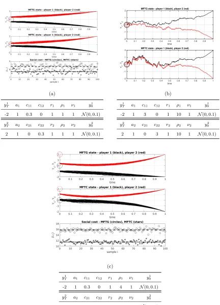
Figure 1 numerical simulations of MFTG and MFTC are presented. In (a), the two players have identical preferences, but different terminal conditions. The situation is symmetric in the sense that we expect the realized paths of player 1 reflected through the line y = 0 to be approximately paths of player 2. In (c), preferences are asymmetric and as a consequence, the realized paths are not each others mirrored images.

The central planner in a MFTC uses more information than a single player does. In fact, in our example, γi,j(t) = 0 when i 6= j in the MFTG. The interpretation is that in the game, player i does not care about player −i’s noise, only its mean state. For the central planner however, γi,j is not identically zero for i6=j. This can be observed in (b), where the central planner makes the player states evolve under some common noise.

In (c) we see an interesting contrast between the MFTG and the MFTC. Player 1 (black) feels no attraction to player 2 (ρ1 = 0) while player 2 is attracted to the mean position of player 1 (ρ2>0). In the game, player 1 travels on the straight line from (t, y)≈(0,−1) to its terminal position (t, y) = (1,−2). Player 2, on the other hand, deviates far from its preferred initial position at time t = 0, only to be in the proximity of player 1. In the MFTC, the central planner makes player 1 linger around y = 0 for some time, before turning south towards the terminal position. The result is less movement movement by player 2. Even though player 1 pays a higher individual cost, the social cost is reduced by approximately 33%. Thesocial cost

J is approximated by

J(u1, u2)≈ 1

N N X

i=1

j(ωi), (5.17)

where j(ωi) =P2 j=1

RT

0 f

j

t(ωi)dt+hj(ωi). In (a) and (c), the outcomes of j (circles for

equi-librium control, stars for optimal control) are presented along with the approximation of J

(dashed lines) forN = 100. The optimal control yields the lower social cost in both cases. This is expected, the general inefficiency of Nash equilibria in nonzero-sum games is well known [16]. The price of anarchy quantifies the inefficiency due to non-cooperation, see for static games [22, 23], for differential games [4] and for linear-quadratic mean-field type games [20]. The price of anarchy in mean-field games has been studied recently in [13, 11]. It is defined as the largest ratio between social cost for an equilibrium (MFTG) to the optimal social cost (MFTC),

P oA:= sup

(ˆu1·,uˆ2·) MFTG equilibrium

J(ˆu1·,uˆ2·)

min

ui

·∈Ui,i=1,2

J(u1

·, u2·)

. (5.18)

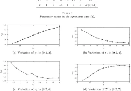
Taking the parameter set of (a) as a point of reference, see Table 1, we vary one parameter at the time and study P oA. The result is presented in Figure 2. In the intervals studied,P oA

is increasing in ρi and T and decreasing in νi and ri. The reason is that the players become

(a)

yT1 a1 c11 c12 r1 ρ1 ν1 y10

-2 1 0.3 0 1 1 1 N(0,0.1)

yT2 a2 c21 c22 r2 ρ2 ν2 y20

2 1 0 0.3 1 1 1 N(0,0.1)

0 0.1 0.2 0.3 0.4 0.5 0.6 0.7 0.8 0.9 1

time -2

-1 0 1 2

Y1

, Y

2

MFTG state - player 1 (black), player 2 (red)

0 0.1 0.2 0.3 0.4 0.5 0.6 0.7 0.8 0.9 1

time -2

-1 0 1 2

Y1

, Y

2

MFTC state - player 1 (black), player 2 (red)

(b)

yT1 a1 c11 c12 r1 ρ1 ν1 y01

-2 1 3 0 1 10 1 N(0,0.1)

yT2 a2 c21 c22 r2 ρ2 ν2 y02

2 1 0 3 1 10 1 N(0,0.1)

(c)

y1

T a1 c11 c12 r1 ρ1 ν1 y01

-2 1 0.3 0 1 4 1 N(0,0.1)

y2

T a2 c21 c22 r2 ρ2 ν2 y02

2 1 0 0.3 1 0 1 N(2,0.1)

y1T a1 c11 c12 r1 ρ1 ν1 y01

-2 1 0.3 0 1 1 1 N(0,0.1)

y2T a2 c21 c22 r2 ρ2 ν2 y02

2 1 0 0.3 1 1 1 N(0,0.1)

Table 1

Parameter values in the symmetric case (a).

0 0.5 1 1.5 2

2

1.04 1.06 1.08 1.1 1.12

PoA

(a) Variation ofρ2 in [0.2,2].

0 0.5 1 1.5 2 2.5 3 3.5 4

r

2 1.05

1.06 1.07 1.08 1.09 1.1

PoA

(b) Variation ofr2 in [0.2,4].

0 0.5 1 1.5 2 2.5 3 3.5 4

1 1.065

1.07 1.075 1.08 1.085 1.09

PoA

(c) Variation ofν1 in [0.2,4].

0 0.5 1 1.5 2

T

1 1.02 1.04 1.06 1.08 1.1

PoA

(d) Variation ofT in [0.2,2].

Fig 2:Numerical approximations (N = 5000) of the price of anarchyP oA.

6. Concluding remarks

Mean-field type games with backward stochastic dynamics, where the coefficients are allowed to depend on the marginal distributions of the player states, have been defined in this paper. Under regularity assumptions existence of a Nash equilibrium is shown, and a verification theorem is proven. In linear-quadric examples, the player behavior in the MFTG is compared to the centrally planned solution in the MFTC, which minimizes social cost. The efficiency of the MFTG Nash equilibrium, quantified by the price of anarchy, and its dependence on problem parameters is studied in the linear-quadratic case.

types of information structures, such as perfect/partial state- and/or law feedback controls, lagged or noise-perturbed controls are of applied interest. Also, both players have perfect information about each other. This can be relaxed to partial information of the states/laws, as well as a treatment of dependencies on the full state-control distribution.

Appendix A: Differentiation and approximation of measure-valued functions

Derivatives of measure-valued functions will be defined with the lifting technique, outlined for example in [8, 10, 12]. Consider the functionf :P2(Rd)→R. We assume that our probability

space is rich enough, so that for every µ ∈ P2(Rd), there exists a square-integrable random

variable X whose distribution is µ, i.e. µ = L(X). For example, ([0,1],B([0,1]), dx) has this property. Then we may writef(µ) =:F(X) and we can differentiateF in Fr´echet-sense when-ever there exists a continuous linear functional DF[X] :L2(F;Rd)→Rsuch that

F(X+Y)−F(X) =E[DF[X]Y] +o(kYk2) =:DYf(µ) +o(kYk2), (A.1)

where kYk2

2 := E[Y2]. DYf(µ) is the Fr´echet derivative off at µ, in the directionY and we

have that

DYf(µ) =E[DF[X]Y] =: lim

t→0

E[F(X+tY)−F(X)]

t , Y ∈L

2_(F;

Rd), µ=L(X). (A.2)

By Riesz’ Representation Theorem, DF[X] is unique and it is known [8] that there exists a Borel function ϕ[µ] :Rd→Rd, independent of the version of X, such thatDF[X] =ϕ[µ](X).

Therefore, withµ0 =L(X0) for some random variableX0, (A.1) can be written as

f(µ0)−f(µ) =E[h[X](X0), X0−X] +o(kX0−Xk2), ∀X0∈L2(F;Rd). (A.3)

We denote ∂µf(µ;x) :=h[µ](x), x∈Rd,∂µf(L(X);X) =:∂µf(L(X)), and we have the

inden-tity

DF[X] =h[L(X)](X) =∂µf(L(X)). (A.4)

Example 1.If f(µ) = (R

Rdxdµ(x)) 2 _then

lim

t→0

E[X+tY]2−E[X]2

t =E[2E[X]Y], (A.5)

and ∂µf(µ) = 2R

Rdxdµ(x). Example 2.If f(µ) =R

Rdxdµ(x) then∂µf(µ) = 1.

The Taylor approximation of a measure-valued function is given by (A.3), and we will write

f(L(X0))−f(L(X)) =E∂µf(L(X))(X0−X)

+o(kX0−Xk₂). (A.6) Assume now thatf takes another argument, ξ. Then

f(ξ,L(X0))−f(ξ,L(X)) =E

h

∂µf(ξ,eL(X);X)(X0−X) i

where the expectation isnot taken over the tilded variable. Note thatPX is deterministic.

In situations where the expected value is taken only over the directional argument of∂µf, we will write

E

h

∂µf(ξ,eL(X);X)(X0−X) i

=:E(∂µf(ξ,L(X)))∗(X0−X)

. (A.8)

The expected value in (A.7) is a random quantity because ofξe. Taking another expected value,

and changing the order of integration, leads to

E

h

e

E[∂µf(ξ,eL(X);X)](X0−X) i

, (A.9)

where the tilded expectation is taken only over the tilded variable. The notation for this will be

e

E[∂µf(ξ,eL(X);X)] =:E[

∗

(∂µf(ξ,L(X)))]. (A.10)

Appendix B: Proofs

Lemma 3.1

Let

ebi_t:=

2

X

j=1

n

∂yjˆbi_tYe_tj +E h

(∂µjˆbi_t)∗Ye_tj io

+ 2

X

j,k=1

∂_zj,kˆbi_tZe_ti,j, (B.1)

then Ye_ti = −

RT

t ebi_s+δ₁bi(s)1_Eε(s)ds−

P2

j=1

RT

t Ze i,j

s dWs. An application of Ito’s formula to

|Ye_t1|2+|Ye_t2|2 yields

2

X

i=1

|Ye_ti|2+

Z T

t

2

X

i,j=1

kZe_si,jk2_Fds=

Z T t 2 2 X i=1

hYe_si,ebi_s+δ₁bi(s)1_Eε(s)ids

+ 2 X i,j=1 Z T t

hYe_si,Ze_si,jdW_sji.

(B.2)

Let D denote the largest bound for all the derivatives of b1 and b2 present. By Jensen’s and Young’s inequalities,

2 2

X

i=1

hYe_si,ebi_si ≤

2

X

i=1

n

(6D+ 16D2)|Ye_si|2+ 2DE[|Ye_si|2] o +1 2 2 X i,j=1

kZe_si,jk2_F. (B.3)

The stochastic integrals in (B.2) are local martingales and vanish under an expectation [27]. Therefore, withK0 := 8D+ 16D2,

E   2 X i=1

|Ye_si|2+

1 2 2 X i,j=1 Z T t

kZe_si,jk2_F ds 

≤K0

Z T t E " ₂ X i=1

|Ye_si|2 # ds + 2 Z T t E " ₂ X i=1

hYe_si, δ₁bi(s)1_Eε(s)i #

ds.

Letτ ∈[0, T], then

sup (T−τ)≤t≤T

K0 Z T t E " ₂ X i=1

|Ye_si|2 #

ds≤K0δ sup

(T−τ)≤t≤T

E

" ₂ X

i=1

|Ye_si|2 #

. (B.5)

and by H¨older’s and Young’s inequalities,

sup (T−τ)≤t≤T

Z T t E " ₂ X i=1

hYe_si, δ₁bi(s)1_Eε(s)i #

ds

≤ sup (T−τ)≤t≤T

Z T t 2 X i=1 E h

|Ye_si|2 i1/2

E|δ1bi(s)1Eε(s)|

21/2 ds ≤ 2 X i=1 ( sup (T−τ)≤t≤T

E

h

|Ye_si|2 i1/2

)

Z T

T−τ

E|δ1bi(s)|2

1/2

1Eε(s)ds

≤ 2 X i=1 δ 2 ( sup (T−τ)≤t≤T

E

h

|Ye_si|2 i

)

+ 1 2δ

Z T

T−δ

E|δ1bi(s)|2

1/2

1Eε(s)ds

2

.

(B.6)

By assumption 5 and the definition ofU1_{, we have for some K} 1 >0,

1 2δ

Z T

T−δ

E|δ1bi(s)|2

1/2

1Eε(s)ds

2

≤K1ε2 (B.7)

Plugging (B.5) and (B.6) into (B.4) yields

sup (T−δ)≤t≤T

E



(1−(K0+ 1)δ)

2

X

i=1

|Ye_ti|2+

1 2 2 X i,j=1 Z T t

kZe_si,jk2_F ds 

≤K1ε2. (B.8)

Forδ <(K0+ 1)−1, we conclude that

sup (T−δ)≤t≤T

E   2 X i=1

|Ye_ti|2+

2

X

i,j=1

Z T

t

kZe_si,jk2_F ds 

≤K2ε2, (B.9)

where K2 > 0 depends on δ, the bound D, the Lipschitz coefficient of bi and the integration bound in the definition ofU1_{. The steps above can be repeated for the intervals [T−2δ, T−δ],} [T−3δ, T−2δ], etc. until 0 is reached. After a finite number of iterations, we have

sup 0≤t≤TE





2

X

i=1

|Ye_ti|2+

2

X

i,j=1

Z T

t

kZe_si,jk2_F ds 

≤K3ε2, (B.10)

Lemma 3.2

Integration by parts yields

E   2 X j=1 e Y₀jp1₀,j



=−E

  Z T 0 2 X j=1 e

Y_tjdp1_t,j+p1_t,jdYe_tj+dhYe_tj, p1,jitdt 

. (B.11)

Assume thatdp1_t,j =β_tjdt+σ_tj,1dW_t1+σj,_t2dW_t2, then

2

X

i=1

e

Y_tidp1_t,i+p1_t,idYe_ti+dhp1,i,Yeii_t=

2

X

i=1

"

e Y_ti

β_tidt+σi,_t1dW_t1+σ_ti,2dW_t2

+p1_t,i

2

X

j=1

(

∂_yjˆbi_tYe_tj+_E h

(∂_µjˆbi_t)∗Ye_tj i

+ 2

X

k=1

∂_zj,kˆbi_tZe_tj,k )

+δ1bi(t)IEε(t)

!

+σi,_t1Ze i,1

t +σ

i,2

t Ze i,2

t #

dt+ (. . .)dW_t1+ (. . .)dW_t2.

(B.12)

Thus the lemma is equivalent to that, under expectations, we have

−E " Z T 0 ( e

Y_t1β_t1+Ye_t2β_t2

+Ye_t1 n

p1_t,1∂y1ˆb1_t+p1_t,2∂_y1ˆb2_t +_E h

∗

(∂µ1ˆb1_t)p1_t,1 i

+E

h

∗

(∂µ1ˆb2_t)p1_t,2 i o

+Ye_t2 n

p1_t,1∂_y2ˆb1_t+p1_t,2∂_y2ˆb2_t +_E h_∗

(∂_µ2ˆb1_t)p1_t,1 i

+E

h_∗

(∂_µ2ˆb2_t)p1_t,2 i o

+ (p1_t,1∂z1,1ˆb1_t+p1_t,2∂_z1,1ˆb2_t +σ_t1,1)Ze_t1,1+ (p1_t,1∂_z1,2ˆb1_t +p1_t,2∂_z1,2ˆb2_t +σ_t1,2)Ze_t1,2

+ (p1_t,1∂z2,1ˆb1_t+p1_t,2∂_z2,1ˆb2_t +σ_t2,1)Ze_t2,1+ (p1_t,1∂_z2,2ˆb1_t +p1_t,2∂_z2,2ˆb2_t +σ_t2,2)Ze_t2,2

+ (p1_t,1δ1b1(t) +pt1,2δ1b2(t))IEε(t)

) dt # =E " Z T 0 2 X i=1 e Y_ti

n

∂_yifˆ_t1+_E

h

∗

(∂_µifˆ_t1)

io

−p1_t,iδ1bi(t)IEε(t)

dt

#

.

(B.13)

We match coefficients and get

β_tj =−p1_t,1∂_yjˆb1_t+p1_t,2∂_yjˆb2_t +_E

h_∗

(∂_µiˆb1_t)p1_t,1

i

+E

h_∗

(∂_µiˆb2_t)p1_t,2

i

+∂yjˆb1_t +_E

h

∗

(∂µjˆb1_t)

i

=−n∂_yjHˆ_t1+_E

h_∗

(∂_µjHˆ_t1

io ,

σ_tj,k =−p1_t,1∂_zj,kbˆ1_t +p1_t,2∂_zj,kˆb2_t

.

Linear-quadratic MFTG - derivation of ODE system

Under the ansatz, the adjoint equation is

dpi,i_t =

n

(qi,i(t) +qi,i_e (t)) ˆY_ti+ (_eqi,i(t) + ¯qi,i(t))E[ ˆYti]

(si,1(t) +si,2(t)¯si,i(t)) ˆYt−i+ (¯si,−i(t) + ¯sEi,1+ ¯si,E2(t))E[ ˆYt−i] o

dt

=:

n

Qi(t) ˆY_ti+ ¯Qi(t)E[ ˆYti] +Si(t) ˆY

−i

t + ¯Si(t)E[ ˆY

−i

t ]

o dt

=nQi(t)

αi(t)pi,it + ¯αi(t)E[pi,it ] +βi(t)p−ti,−i+ ¯βi(t)E[p−ti,−i]

+γi,1(t)W_t1+γi,2Wt2+θi(t)

+ ¯Qi(t)

(αi(t) + ¯αi(t))E[pi,it ] + (βi(t) + ¯βi(t))E[pt−i,−i] +θi(t)

+Si(t)

α−i(t)p−ti,−i+ ¯α−i(t)E[pt−i,−i] +β−i(t)pi,it + ¯β−i(t)E[pi,it ]

+γ−i,1Wt1+γ−i,2Wt2+θ−i(t)

+ ¯Si(t)

(α−i(t) + ¯α−i(t))E[p−ti,−i] + (β−i(t) + ¯β−i(t))E[pi,it ] +θ−i(t) o

dt

=

n pi,i_t

Qi(t)αi(t) +Si(t)β−i(t)

+E[pi,it ]

Qi(t) ¯αi(t) + ¯Qi(t)(αi(t) + ¯αi(t)) +Si(t) ¯β−i(t) + ¯Si(t)(β−i(t) + ¯β−i(t))

+p−_ti,−i

Qi(t)βi(t) +Si(t)α−i(t)

+E[p−ti,−i]

Qi(t) ¯βi(t) + ¯Qi(t)(βi(t) + ¯βi(t)) +Si(t) ¯α−i(t) + ¯Si(t)(α−i(t) + ¯α−i(t))

+W_t1(Qi(t)γi,1(t) +Si(t)γi,2(t)) +Wt2(Qi(t)γi,2+Si(t)γ−i,2) +θi(t)(Qi(t) + ¯Qi(t)) +θ−i(t)(Si(t) + ¯Si(t))

o dt

=:npi,i_t Pi(t) +E[pi,it ] ¯Pi(t) +p

−i,−i

t Ri(t) +E[p

−i,−i t ] ¯Ri(t)

+W_t1Φi(t) +W_t2Ψi(t) +θi(t)(Qi(t) + ¯Qi(t)) +θ−i(t)(Si(t) + ¯Si(t)) o

dt,

(B.15) and the expected value ofpi,i· solves

d(E[pi,it ]) = n

E[pi,it ](Pi(t) + ¯Pi(t)) +E[p

−i,−i

t ](Ri(t) + ¯Ri(t))

+θi(t)(Qi(t) + ¯Qi(t)) +θ−i(t)(Si(t) + ¯Si(t)) o

dt.

(B.16)

The initial conditionspi,i₀ , E[pi,i0 ], p

−i,−i

0 , E[p

−i,−i

and using (B.15)-(B.16), we get

dYˆ_ti=α˙i(t)pi,it + ˙¯αi(t)E[pi,it ] + ˙βi(t)p−ti,−i+ ˙¯βi(t)E[p−ti,−i]

+ ˙γi,1(t)W_t1+ ˙γi,2(t)W_t2+ ˙θi(t)

dt

+αi(t)dpi,it + ¯αi(t)d(E[pi,it ]) +βi(t)dp−ti,−i+ ¯βi(t)d(E[p−ti,−i])

+γi,1(t)dW_t1+γi,2(t)dW_t2

=

n pi,i_t

˙

αi(t) +αi(t)Pi(t) +βi(t)Ri(t)

+E[pi,it ]

˙¯

αi(t) +αi(t) ¯Pi(t) + ¯αi(t)(Pi(t) + ¯Pi(t))

+βi(t) ¯R−i(t) + ¯βi(t)(R−i(t) + ¯R−i(t))

+p−_ti,−i

˙

βi(t) +αi(t)Ri(t) +βi(t)P−i(t)

+E[p−ti,−i]

˙

βi(t) +αi(t) ¯Ri(t) + ¯αi(t)(Ri(t) + ¯Ri(t))

+βi(t) ¯P−i(t) + ¯βi(t)(P−i(t) + ¯P−i(t))

+W_t1γ˙i,1+αi(t)Φi(t) +βi(t)Φ−i(t)

+W_t2γ˙i,2+αi(t)Ψi(t) +βi(t)Ψ−i(t)

+

˙

θi(t) +θi(t) (αi(t) + ¯αi(t))(Qi(t) + ¯Qi(t)) + (βi(t) + ¯βi(t))(S−i(t) + ¯S−i(t))

+θ−i (αi(t) + ¯αi(t))(Si(t) + ¯Si(t)) + (βi(t) + ¯βi(t))(Qi(t) + ¯Qi(t))

o

dt

+γi,1(t)dWt1+γi,2dWt2.

(B.17) We can now match these dynamics with the true state dynamics and we get the system of ODEs (5.10) andγi,j(t) = ˆZ_ti,j.

References

[1] Andersson, D. and Djehiche, B. [2011], ‘A maximum principle for SDEs of mean-field type’,Applied Mathematics & Optimization 63(3), 341–356.

[2] Aurell, A. and Djehiche, B. [2018a], ‘Mean-field type modeling of nonlocal crowd aversion in pedestrian crowd dynamics’,SIAM Journal on Control and Optimization 56(1), 434– 455.

[3] Aurell, A. and Djehiche, B. [2018b], ‘Modeling tagged pedestrian motion: a mean-field type control approach’,arXiv preprint arXiv:1801.08777.

[4] Ba¸sar, T. and Zhu, Q. [2011], ‘Prices of anarchy, information, and cooperation in differ-ential games’,Dynamic Games and Applications1(1), 50–73.

[5] Bensoussan, A., Frehse, J., Yam, P. et al. [2013], Mean field games and mean field type control theory, Vol. 101, Springer.

[7] Buckdahn, R., Djehiche, B., Li, J., Peng, S. et al. [2009], ‘Mean-field backward stochastic differential equations: a limit approach’,The Annals of Probability37(4), 1524–1565. [8] Buckdahn, R., Li, J. and Ma, J. [2016], ‘A stochastic maximum principle for general

mean-field systems’,Applied Mathematics & Optimization 74(3), 507–534.

[9] Buckdahn, R., Li, J. and Peng, S. [2009], ‘Mean-field backward stochastic differential equations and related partial differential equations’,Stochastic Processes and their Appli-cations119(10), 3133–3154.

[10] Cardaliaguet, P. [2010], Notes on mean field games, Technical report.

[11] Cardaliaguet, P. and Rainer, C. [2018], ‘On the (in) efficiency of MFG equilibria’, arXiv preprint arXiv:1802.06637.

[12] Carmona, R. and Delarue, F. [2018], Probabilistic Theory of Mean Field Games with Applications I-II, Springer.

[13] Carmona, R., Graves, C. V. and Tan, Z. [2018], ‘Price of anarchy for mean field games’, arXiv preprint arXiv:1802.04644.

[14] Chen, Z. and Epstein, L. [2002], ‘Ambiguity, risk, and asset returns in continuous time’, Econometrica70(4), 1403–1443.

[15] Djehiche, B., Tcheukam, A. and Tembine, H. [2017], ‘Mean-field-type games in engineer-ing’,AIMS Electronics and Electrical Engineering 1(1), 18–73.

[16] Dubey, P. [1986], ‘Inefficiency of nash equilibria’, Mathematics of Operations Research 11(1), 1–8.

[17] Duffie, D. and Epstein, L. G. [1992a], ‘Asset pricing with stochastic differential utility’, The Review of Financial Studies5(3), 411–436.

[18] Duffie, D. and Epstein, L. G. [1992b], ‘Stochastic differential utility’,Econometrica: Jour-nal of the Econometric Societypp. 353–394.

[19] Duffie, D., Geoffard, P.-Y. and Skiadas, C. [1994], ‘Efficient and equilibrium allocations with stochastic differential utility’, Journal of Mathematical Economics23(2), 133–146. [20] Duncan, T. E. and Tembine, H. [2018], ‘Linear–quadratic mean-field-type games: A direct

method’,Games9(1), 7.

[21] El Karoui, N., Peng, S. and Quenez, M. C. [1997], ‘Backward stochastic differential equa-tions in finance’,Mathematical finance 7(1), 1–71.

[22] Koutsoupias, E. and Papadimitriou, C. [1999], Worst-case equilibria,in ‘Annual Sympo-sium on Theoretical Aspects of Computer Science’, Springer, pp. 404–413.

[23] Koutsoupias, E. and Papadimitriou, C. [2009], ‘Worst-case equilibria’, Computer science review3(2), 65–69.

[24] Li, J. and Min, H. [2016], ‘Controlled mean-field backward stochastic differential equations with jumps involving the value function’, Journal of Systems Science and Complexity 29(5), 1238–1268.

[25] Li, X., Sun, J. and Xiong, J. [2016], ‘Linear quadratic optimal control problems for mean-field backward stochastic differential equations’, Applied Mathematics & Optimization pp. 1–28.

[26] Papadimitriou, C. [2001], Algorithms, games, and the internet, in ‘Proceedings of the thirty-third annual ACM symposium on Theory of computing’, ACM, pp. 749–753. [27] Pardoux, ´E. [1999], Bsdes, weak convergence and homogenization of semilinear PDEs,in

‘Nonlinear analysis, differential equations and control’, Springer, pp. 503–549.

equation’,Systems & Control Letters 14(1), 55–61.

[29] Tang, M. and Meng, Q. [2016], ‘Linear-quadratic optimal control problems for mean-field backward stochastic differential equations with jumps’,preprint arXiv:1611.06434. [30] Yong, J. [2010], ‘Forward-backward stochastic differential equations with mixed

initial-terminal conditions’, Transactions of the American Mathematical Society 362(2), 1047– 1096.