A Parametric Bayesian Approach in Density Ratio
Estimation
Abdolnasser Sadeghkhani1,∗ , Yingwei Peng2and C. Devon Lin3
1 Department of Mathematics, Brock University, St. Catharines, ON, Canada; [email protected] 2 Departments of Public Health Sciences, Queen’s University, ON, Canada; [email protected] 3 Department of Mathematics & Statistics, Queen’s University, ON, Canada [email protected]; * Correspondence: [email protected];
Abstract:This paper considers estimating the ratio of two distributions with different parameters and common supports. We consider a Bayesian approach based on the Log–Huber loss function which is resistant to outliers and useful to find robust M-estimators. We propose two different types of Bayesian density ratio estimators and compare their performance in terms of Bayesian risk function with themselves as well as the usual plug–in density ratio estimators. Some applications such as classification and divergence function estimation are addressed.
Keywords:Bayes estimator, Bregman divergence, Density ratio, Exponential family, Log–Huber loss.
1. Introduction
The problem of estimating the ratio of two densities appears in many areas of statistical and computer science. The density ratio estimation (DRE) is widely considered to be the most important factor in the machine learning and information theory. Sugiyama et al. in a series of papers (e.g. 2009, 2011) developed the DRE in different statistical data analysis problems. Some useful applications of the DRE are as follows: non–stationary adaptation (Sugiyama and Müller 2005 and Quiñonero-Candela et al., 2009), variable selection (Suzuki et al., 2009), dimension reduction (Suzuki and Sugiyama, 2010), conditional density estimation (Sugiyama et al., 2010), outlier detection (Hido et al., 2008) among others. This paper addresses cases when the density belongs to the parametric distributions (e.g., exponential family of distributions). Parametric methods are usually favourable thanks to existence of closed forms (mostly, simple and explicit formulas) and hence help to enhance computational efficiency.
Recently several estimators of the ratio of two densities have been proposed. One of the simplest approaches to estimate density ratiop/q, wherepandqare two probability density (or mass) functions (PDF or PMF), is called “plug–in", which the ratio of the estimated densities is computed. Alternatively, one can estimate the ratio of two densities directly. Several approaches have been explored recently to estimate the ratio including moment matching approach (Gretton et al., 2009) and density matching approach (Sugiyama, 2008). There exists other work such as Nguyen (2010) and Deledalle (2017) which studied the application of DRE in estimating Kullback–Leibler (KL) divergence (or more generally
α–divergence function, also known as f–divergence) and vice versa. The main objective of this paper
is to address the Bayesian parametric estimation with some commonly used loss functions for the ratio ofp/qand to compare the proposed estimators with other estimators in the literature.
The remainder of the paper is organized as follows. In Section 2, we discuss the methodology of the DRE and introduce some useful definitions and related examples. Section 3 discusses how to find a Bayesian DRE under several loss functions for any arbitrary prior density on the parameter, and provides some interesting examples from the exponential families. In Section 4 we study some of the DRE applications. Se. Some numerical illustrations for considering the efficiency of the proposed DRE’s are given in Section 5. Finally, we make some concluding remarks in Section 6.
2. Density ratio estimation for exponential distribution family
LetX|ηandY|γbe conditionally independent multivariate random variables p(x|η) =h(x)exp
n
η>s(x)−κ(η)
o
, (1)
q(y|γ) =h(y)exp
n
γ>s(y)−κ(γ)
o
, (2)
where η, γ ∈ Rd are natural parameters, s(·) is a sufficient statistic, and κ(·) = logc(·) is the
log–normalizer, which ensures that the distribution integrates to one. Consider the problem of estimating the density ratio
r(t;η,γ) = p(t|η)
q(t|γ), (3)
which obviously is proportional to exp
(η−γ)>s(t) . So one can merge two natural parametersη
andγinto one single parameterβ= η−γ(it can be a vector), and write the density ratio in (3) as
follows
r(t;θ) =exp
n
α+β>s(t)
o
, (4)
where α = κ(γ)−κ(η), and θ = (α,β>) are parameters of interest. Note that sincer(t;θ)itself
belongs to the exponential family, the normalization termαcan be considered as−logN(β), where N(β) =R q(t)expβ>s(t) dt, that guaranteesR q(t|γ)r(t;θ)dt=1 and henceq(t)r(t;θ)becomes a
valid PDF (PMF).
For instance, suppose two normal densitiesp(t|µ1,σ12) =N(t| µ1,σ12)andq(t| µ2,σ22) =N(t| µ2,σ22). They are corresponding to (1) and (2) respectively. One can easily verify thatη= (µ1
σ12,
−1 2σ12)
>,
γ= (µ2 σ22,
−1 2σ22)
>,s(t) = (t,t2)>and
κ(η) = µ
2 1
2σ12 +logσ
2
1,γ(η) =
µ22
2σ22 +logσ
2
2, and so according to (4),
we haveα=logσσ1
2 +
µ21
2σ12 − µ22
2σ22 andβ=
µ2
σ22 − µ1
σ21,
1 2σ12 −
1 2σ22
>
.
Another interesting point is the relationship between DRE and probabilistic classification problem (Sugiyama et al. 2012 c ) SupposeZ={0, 1}is a binary response variable which shows whether an observationtis drown from eitherp(·|η)(sayZ=0) orq(·|γ)(sayZ =1). In such a classification
problem the logistic model has the form
P(Z=1|t) = exp(β0+β
>t) 1+exp(β0+β>t),
and consequently,P(Z=0|t) = 1+exp(β1
0+β>t)and
P(Z=1|t)
P(Z=0|t) =exp(β0+β
>
t). (5)
Lettingπ =P(Z=1) = R P(Z=1|t)p(t)dtandp(t) =P(t| Z=0)andq(t) =P(t| Z=1), we
have
p(t) = exp(β0+β >t) (1+exp(β0+β>t))π, q(t) = p(t)
and hence
p(t)
q(t) = 1−π
π exp(β0+β
>) = exp
α+log1−π π +β
>t ,
which has indeed form of exp(α+β>t)withα=β0+log1−ππ and hence has a density ratio model in (4).
However if our responseZ={0, 1, . . . ,m−1}, we can extend equation (5) to the multinomial logit model, and we have
P(Z=k|t)
P(Z=0|t) =exp(β0k+β
>
kt), k=1, . . . ,m−1 . (6)
Analogously, letting Pk(t) = P(t | Z = k) and πk = P(Z = k) for k = 1, . . . ,m−1, we have
Pk(t)
P0(t) =exp(αk+β >
k), withαk=β0k+log 1−∑k−1
k=1πk πk .
In fact a conceptually simple solution to the DRE is to estimate separately each of two densities and calculate the ratio. This can be done by replacing the estimators of the parameters into each density. This approach is known as a plug–in density ratio estimation, defined in below
ˆ
rplug(t) =
p(t|ηˆ(t))
q(t|γˆ(t)), (7)
where ˆη(·)and ˆγ(·)are estimates of parameters ofpη(·)andqγ(·)based on a sample of sizenpandnq respectively .
3. Bayesian DRE
Consider the loss function`(θ,δ(t))and its average under long–term (repeated) use ofδ(t), in
estimatingθis called frequentist risk and given by
R(θ,δ) =ET|θ[`(θ,δ)] (8)
=
Z
t
`(θ,δ(t))Pθ(dt), (9)
whereET|θ(·)is the expectation with respect to the arbitrary measurable cumulative density function
(CDF)T∼P(t|θ). Given any prior distributionπ, it is also possible to define theintegrated risk(Bayes risk), which is the frequentist risk averaged over the values ofθaccording to prior distributionπ(θ)
and posterior distributionπ(θ|t).
Eθ|t[R(δ(t),θ)] =
Z
Θ Z
T `(θ,δ(t))π(θ|t)dt dθ. (10) Finally, the Bayes estimator is the minimizer of the Bayes risk (10). It can be shown that the minimizer of the above expression also minimize the posterior risk function and hence is the Bayes estimator (See Lehman and Casella 1998) .
Next, we will address the log–Huber loss and reasons beyond choosing such a loss function, in order to study the efficiency of the DRE.
3.1. Log–Huber’s robust loss
One of the weakness of a squared error loss functionz2, withz = δ−θ, is that it can overly
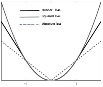
can use the absolute loss function|z|, but since it is not a differentiable function at the origin, Huber (1964), proposed the following function instead
H(z) = (
z2 |z| ≤1
2|z| −1 |z| ≥1 , (11)
which is equivalent to the squared error loss (L2loss) for errors that are smaller than 1, and absolute error loss (L1loss) for larger errors (See Figure1). This loss borrows advantages ofL1andL2losses and does not have their disadvantage. That is, it is not sensitive to the outliers (as opposed toL2) and it is it is everywhere differentiable (as opposed toL1). In practice optimizing the Huber loss (and consequently, Log–Huber) is much faster because it enables us to use standard smooth optimization methods (such as quasi-Newton) instead of linear programming.
In the context of the DRE, we propose takingz=logrrˆ((tt,)
θ)in (11), yields the Log–Huber’s loss function `(rˆ,r) =R(logrrˆ)2dP(t)
The corresponding frequentist risk function to the Log–Huber’s loss function is given by
R(rˆ,θ) =
( R R
(logrrˆ)2dP(x)dP(y) e−1≤ rrˆ ≤e
2R R
|logrrˆ| −1
dP(x)dP(y) 0< rrˆ ≤e−1, rrˆ ≥e, (12) whereθ= (η,γ)and hence the Bayes risk for the Bayesian DRE is given byRπ(rˆ) =Eθ|tR(rˆ,θ), which
is a scalar and a function oft.
Figure 1.Comparison of Huber,L2(least square), andL1(absolute error) loss functions in (11)
Before discussing further on this topic, it is worthwhile to consider the specific cases of Log–L2and Log–L1respectively along with some useful definitions. Here are a definition and a lemma appeared in Nielsen and Nock (2010).
Definition 1. Bregman divergence associated with a real valued strictly convex and differentiable function c(·), is defined by
B(η,γ) =κ(η)−κ(γ)− hη−γ,∇c(γ)i, (13)
whereh·,·iis the inner product and and other notations are similar to equation (1). It can be shown that for all regular exponential families (see, Brwon 1986)κ(·), is strictly convex, and furthermore B(η,γ) =logcc((ηγ))− hη−γ,Eq(s(T))i.
Lemma 1. The Kullback–Leibler (KL) distance between pηand qγin model (1) is equal to Bregman divergence between natural parameters. That is:
where the KL divergence (Kullback–Leibler, 1951), between densities f1and f2, KL(f1,f2) =Ef1logf1/f2.
3.1.1. Log–L2loss function
The Log–L2loss(logz)2, withz= rrˆ, puts a small weight whenever the density ratio estimator ˆr and the true density ratiorare close and proportionately more weight when they are significantly different. Lemma2provides the Bayesian DRE of the density ratiorin (3).
Lemma 2. For any measurable PDF p(· |η)and q(· |γ), the Bayesian DRE of r(t;θ)associated with log–L2
loss function(logrrˆ)2and prior distributionπ(θ)onθ= (η,γ)is given by
ˆ
rπ(t) =exp
n
Eθ|X=t,Y=tKL(p,q)
o
, (14)
and in addition for the natural exponential family model (1) also it can be expressed as
ˆ
rπ(t) =exp
n
Eθ|X=t,Y=tB(η,γ)
o
. (15)
Note thatEθ|X=t,Y=t(·)represents the expectation associated withθ|X=t,Y=t. Proof. For simplicity assume notations ˆrπ(t)andr(t;η,γ)as ˆrandrrespectively.
The Bayesian estimator ˆrin estimatingris the minimizer of the posterior riskEθ|t`(rˆ,r), with`(ˆr,r) = Ep(logrrˆ)2, and therefore, ∂log ˆ∂ rEθ
|t
Ep(log ˆr−logr)2 = 0 implies log ˆrπ(t) = Eθ|tEplogr = Eθ|tKL(p,q). Applying Lemma1and the fact that ∂
2
∂log ˆr2E η|t
Ep(log ˆr−logr)2 ≥ 0, completes the
proof.
An interesting alternative representation of Bayesian DRE from Lemma2is that is the Bayesian DRE can be expressed in terms of the plug–in DRE in (7).
Corollary 1. For any PDF p and q belong to (1) and (2) respectively, the Bayesian DRE of under Log–L2loss
L(rˆ,r) = (logˆrr)2, and prior distributionπ(θ), forθ= (η,γ), is given by
ˆ
rπ(t) =rˆplug(t)H(t), (16)
where,rˆplugis obtained by replacing posterior expectations of unknown parameters given t.
ˆ
rplug(t) =
exp{hs(t),Eη|X=t,Y=tηi −logEη|X=t,Y=tlogc(η)}
exp{hs(t),Eγ|X=t,Y=tγi −logEγ|X=t,Y=tlogc(γ)}}
, (17)
and the correction factor
H(t) = exp{logE
η|X=t,Y=tc(
η)−Eη|X=t,Y=tlogc(η)}
exp{logEγ|X=t,Y=tc(γ)−Eγ|X=t,Y=tlogc(γ)}, (18) Proof. The Bayesian DRE ˆrπ(t)is the minimizer of the posterior risk and
∂ ∂ log ˆrπ
Eη|X=t,Y=t(log ˆrπ−logr)
2 = 0 ,
implies log ˆrπ(t) = Eη|X=t,Y=tlogrπor equivalently,
ˆ
rπ(t) =exp
n
Eη|X=t,Y=tlogr(t)
o
with ∂2 ∂log ˆr2π E
η|X=t,Y=t(log ˆr−logr)2≥0. Therefore
ˆ
rπ(t) =exp
n
Eη|X=tlogpη(t)−Eγ
|Y=tlogq
γ(t)
o
=
expnEη|X=tlogpη(t)
o
exp
Eγ|Y=tlogqγ(t)
= h1(t)exp{ηˆ>(x)s1(t)−logc1(ηˆ(t))}
h2(t) exp{γˆ>(t)s2(t)−logc2(γˆ(t))}
×exp
n
c1(ηˆ1(t))−log\c1(η1)(t)
o
expnc2(ηˆ2(t))−log\c2(η2)(t)
o
=rˆplug(t)H(t), This completes the proof.
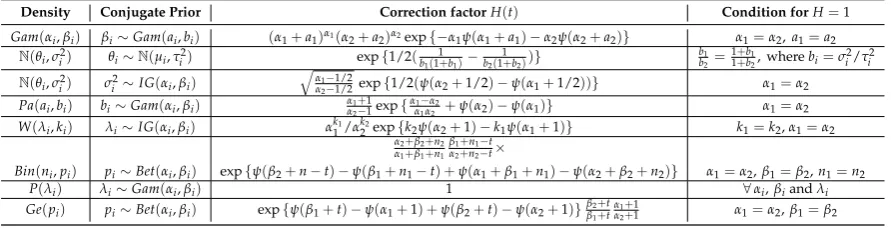
Table 1 explores the correction factorH(·)for certain densities which belong to exponential family associated with log–L2loss. Let the likelihood functions in below with sub indicesi=1, 2 represent the underlying distributions are drawn frompandqaccordingly to (1) and (2) respectively. It is worth noting that posing constraints on the hyper–parameters leads to haveH(t)as a constant function int. In fact,H(t) =1 induces the Bayesian DRE ˆrπcoincides with the plug–in DRE ˆrplug.
Note that the notationψ(α)in below is for a “digamma" function and is given by∂Γ(Γδ()/∂δ δ) . Also, Gam, P, Pa, W and Geo stand for gamma, poisson, pareto, weibull and geometric distributions respectively.
Density Conjugate Prior Correction factorH(t) Condition forH=1
Gam(αi,βi) βi∼Gam(ai,bi) (α1+a1)α1(α2+a2)α2exp{−α1ψ(α1+a1)−α2ψ(α2+a2)} α1=α2,a1=a2 N(θi,σi2) θi∼N(µi,τi2) exp{1/2(b 1
1(1+b1)−
1
b2(1+b2))}
b1 b2=
1+b1
1+b2, wherebi=σ
2
i/τi2
N(θi,σi2) σ2i ∼IG(αi,βi)
q
α1−1/2
α2−1/2exp{1/2(ψ(α2+1/2)−ψ(α1+1/2))} α1=α2 Pa(ai,bi) bi∼Gam(αi,βi) αα12+−11exp{
α1−α2
α1α2 +ψ(α2)−ψ(α1)} α1=α2 W(λi,ki) λi∼IG(αi,βi) αk11/α2k2exp{k2ψ(α2+1)−k1ψ(α1+1)} k1=k2,α1=α2
Bin(ni,pi) pi∼Bet(αi,βi)
α2+β2+n2
α1+β1+n1
β1+n1−t
α2+n2−t×
exp{ψ(β2+n−t)−ψ(β1+n1−t) +ψ(α1+β1+n1)−ψ(α2+β2+n2)} α1=α2,β1=β2,n1=n2
P(λi) λi∼Gam(αi,βi) 1 ∀αi,βiandλi
Ge(pi) pi∼Bet(αi,βi) exp{ψ(β1+t)−ψ(α1+1) +ψ(β2+t)−ψ(α2+1)}ββ2+t
1+t
α1+1
α2+1 α1=α2,β1=β2 Table 1.Correction factorH(t)and conditions whenH(t) =1 associated with log–L2loss
3.1.2. Log–L1loss function
For some larger errors in loss function (12), one needs to consider Log–L1loss function`(r˜,r) = 2|logr˜r| −2 for all ˜r≤r/e, ˜r≥r e. Let ˜rbe the corresponding Bayesian DRE. Similar calculation to Lemma2suggests
˜
rπ(t) =exp
n
Mθ|X=t,Y=tB(η,γ)
o
,
whereMθ|t(·)is the median of the posterior density function θ | t. Similar to Section3.1.1, and
equations (14) and (15), we can write ˜rπ(t) = exp
n
Mθ|X=t,Y=tKL(p,q)
o
which expectations are replaced by medians.
Alike Corollary1we also can express ˜rπ(t)in terms of product of the correction factor and the
plug–in DRE. That is, under Log–L1lossL(r˜,r) =|logrrˆ|, and prior distributionπ(θ), forθ= (η,γ), we have
˜
where the ˜rplug(t)andH0(t)are obtained in the same fashion in (17) and (18) except applying median
Mθ|X=t,Y=t(·)instead ofEη|X=t,Y=t(·). Notice that for instance the results in Table1hold, wherever
the posterior densities turn out to be symmetric about their means (or medians).
3.2. Examples of the Bayesian DRE and some applications
We consider commonly used families of distributions and study the corresponding Bayesian DREs. As we saw in the previous section, the key point is to find the KL divergence between two densities
pandq(or equivalently, Bregman divergence in the cases of distributions belonging to exponential family) and we have a closed-form for the divergence. The following table presents the KL divergence betweenpandq.
Density KL
Np(θi,Σi) 12
h
(θ1−θ2)0Σ2−1(θ1−θ2) +tr(Σ−21Σ1)−p−logdetdet((ΣΣ12))
i
N(θi,σi) 21σ2
2
(θ1−θ2)2+σ12−σ22−12logσ
2 1 σ22
Bet(ai,bi) logBetBet((aa12,b,b12))+ψ(a1)(a1−a2) +ψ(b1)(b1−b2) +ψ(a1+b1)(a2−a1+b2−b1) Gam(ki,λi) (λλ12−1)k1+ (k1−k2)(logλ1+ψ(k1))−log
Γ(k1)λ1k1 Γ(k2)λ2k2
χ2(ki) logΓ
(k2 2) Γ(k1
2)
+12ψ(k22)(k1−k2) Log–N(θi,σi2) 21
σ22
(θ1−θ2)2+σ12−σ22−logσ
2 1 σ22
Ray(σi) 2 logσσ21+σ
2 1−σ22
σ22
Pa(mi,αi) log(mm12)
2−loga2
a1+
a2
a1−1
U(0,θi) log(θθ21)Providedθ2>θ1
Table 2.KL divergence betweenpandq
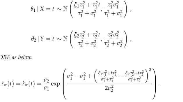
Example 1. Let X|θ1 ∼ N(θ1,σ12)be independent of Y|θ2 ∼ N(θ2,σ22),with the known variances and independent prior distributionsθi ∼N(ξi,τi2)for i=1, 2. Hence the posterior densities are given by
θ1|X=t ∼N ξ1τ
2 1+τ12t
τ12+σ12 , τ12σ12
τ12+σ12
!
,
θ2|Y=t ∼N ξ2τ
2 2+τ22t
τ22+σ22 , τ22σ22
τ22+σ22
!
,
yields the Bayesian DRE as below.
˜
rπ(t) =ˆrπ(t) = σ2
σ1 exp
σ12−σ12+
ξ1σ12+tτ12 σ12+τ12 −
ξ2σ22+tτ22 σ22+τ22
2
2σ22
. (20)
Np(W1(Σ1−1t+V1−1ξ1),W1)andθ2|t∼Np(W2(Σ−21t+V2−1ξ2),W2)with Wi = (Σ−i 1+V −1 i )
−i. Therefore
the Bayesian DRE for the ratio of two multivariate normal densities equals to
1 2
h
(W1(Σ−11t+V −1
1 ξ1)−W2(Σ−21t+V −1
2 ξ2))0Σ−21(W1(Σ−11t+V −1 1 ξ1)
−W2(Σ2−1t+V −1
2 ξ2)0+tr(Σ−21Σ1)− 1 2log
det(Σ1)
det(Σ2)
.
Example 2. Let X|σ12∼Ray(σ12)and Y|σ22∼Ray(σ22)be two independent random variables from Rayleigh distribution with the PDF p(x|σ2) = x
σ2 exp(−
x2
2σ2)for x > 0andσ
2 > 0. The KL divergence between
p(x|σ12)and p(y|σ22)is given in the Table2. Assumingλi=2σi2, and choosing the inverse gamma conjugate prior distribution (IG) with parametersαandβ, with the PDFπ(λ|α,β) = β
α
γ(α)λ
−(α+1)exp(−β
λ)forλ>0, which yields to have the posterior distribution as follows
λi |t∼IG(1+αi,βi+t2). (21)
Therefore the Bayesian DRE for ratio of two Rayleigh densities is the exponential function of the conditional expectation of their KL loss divergence function. That is,
expEλ2|tλ2−Eλ1|tlogλ1+Eλ1|tλ1Eλ2|tλ−1
2 −1
.
By making use of properties ofλ ∼ IG(α,β), such asE(logλ) = logβ−ψ(α), whereψ(α)is a
“digamma" function, the Bayesian DRE under log–L2loss is give by
ˆ
rπ(t) =
β2+t2
β1+t2 exp
α2−α1
α1α2
+ α1
1+α2
β1+t2
β2+t2
−ψ(α2) +ψ(α1)−1
.
Since the median of an inverse gamma distribution does not have a closed form, we cannot express an explicit formula for the Bayesian DRE under log–L1loss function and consequently for the log–Huber loss and they must be calculated iteratively.
The following remarks are some clarification related to Table2and the obtained Bayes estimators in the previous examples in Section.3.2.
Remark 1. The Bayes DRErˆπ(t)is connected to samples X and Y via the posterior densityη| X =t and γ|Y=t.
Remark 2. From Table2it can be seen that the KL divergence between two log–normal PDF’s is the same as in normal distributions, since it is known that KL is invariant under parameter transformations.
Remark 3. Equations (14) and (15) are applicable for not only exponential family but any distributions. The key point is that the nice representation of Bayesian DRE in (16) and (19) are correct based on models (1) and (2). Example 3. Suppose, X∼Uni f orm(0,θ1)is independent of Y∼Uni f orm(0,θ2), withθ1<θ2. It is easy
to check Pareto distribution is conjugate to a uniform. Hence assume thatπ(θi) =αiβαiiθi−(α1+1)forθ≥βi
and i=1, 2, therefore
θi |t∼Pareto(1+αi, max(βi,t))
Moreover, assuming p and q are the PDF’s of X and Y respectively, therefore, KL(p,q) =logθ2−logθ1(see
Table2). Employing the fact that transformationlog(z/b)has exponential distribution with mean of a, given Z∼Pareto(a,b), and henceEZlogZ=a+logb, after some calculation we have the Bayes DRE associated with log–L2
ˆ
rπ(t) =
max(β2,t)
max(β1,t)
4. Other applications
Here, we discuss some of other applications of DRE method.
1. Estimatingα–divergence function between two probability densities:
A discrepancy measure between densitiespηandqγapplicable to the class of Ali-Silvey (1966)
distance also known asα–divergence (Csiszàr, 1967) is given by
`α(p(· |η),q(·|γ)) =
Z
Rd
hα
p(t|η) q(t|γ)
d P(t|γ), (22)
where
hα(z) =
4
1−α2(1−z
−(1+α)/2) for|α| ≤1
−log(z)/z forα=−1
log(z) forα=1.
Note that some of the notable divergence functions say, Kullback–Leibler, reverse Kullback–Leibler (RKL) and Hellinger divergence functions correspond toα = 1,−1 and 0
respectively and belong to this class. So, ifr(t)is estimated by ˆrπ(t)under log–L2(or ˜rπ(t) under
log–L1losses ), then applying the Monte–Carlo approximations method, theα–divergence is
also estimated by
dα(t) =1/n
n
∑
i=1
hα(rˆπ(ti)), (23)
wheretiare drown fromp(· |η). It is worthwhile to note that there are other work in order to
estimate theα–divergence loss function (eg. Póczos and Schneider 2010) but our estimator in
(23), is based on the Bayesian parametric method based on the DRE. Next section we show the performance of the proposal estimatordα.
2. plug–in type estimation of the density ratio under KL loss function
Consider the plug–in density estimator, say,pηˆ(t)for estimatingpηin the exponential family (1),
based on the KL loss. We have
KL(p(t|η),p(t|ηˆ)) =
Z
logp(η|t)
p(t|ηˆ)P(t|η)dt =
Z
p(t|ηˆ)log exp{hη,s(t)i −c(η)} exp{hηˆ(t),s(t)i −c(ηˆ(t))}dt
= hη−ηˆ(t),Eps(T)i −(c(η)−c(ηˆ(x))
= hη−ηˆ(t), ∂c(η)
∂ η i −(c(η)−c(ηˆ(t)). (24)
Next, finding the plug–in density estimatorp(t, ˆη(t))that minimizes KL loss, is equivalent to
find the point estimator ˆη(t), which minimizes the posterior expectation associated with the loss
function in (24). Therefore, ∂ ∂ηˆE
η|tKL(p(t|η),p(t|ηˆ)) =0, impliesc
1(ηˆ) =Eη|t c(ηη)and hence
the Bayes estimator ofηis given by
ˆ
η1(t) =c−11
Eη|tc1(η) η
. (25)
Similar arguments can be applied toqγˆ(t)for estimatingqγin the exponential family (2), and we
have,
ˆ
γ2(y) =c−21
Eγ|tc2(γ) γ
By setting the case when the both densities follow the identical distribution from (1) (for instance the ratio of two normal or two Poisson, etc.), substituting the Bayes estimators obtained in (25) and (26) into the plug–in estimator ofr(t), gives
ˆ
r(t) =exp{(ηˆ1(t)−ηˆ2(t))>s(t)−(c1(ηˆ1(t)−c2(ηˆ2(t))}. (27) Note that ˜r(t)can be obtained similarly by replacing posterior medians ˜ηiinstead of posterior expectations ˆηifori=1, 2, in above.
5. Numerical illustrations
We conclude this section with some numerical illustrations of log–Huber risk performance of the Bayesian and plug–in when bothpandqare two normal models (belong to model1and2) with a common location parameterθ. We show that the performance of plug–in and Bayes are quite similar
and by selecting the hyper–parameters these two density ratio estimators coincide and hence have the same frequentist risk. We start with comparing risk performance under the log–L2first and then extend them log–Huber loss.
Figure2exhibits the frequentist risk performance of the plug–in DRE ˆrplugand the Bayes DRE ˆrπ
under log–L2for all possible values ofθusing Corollary1.
-1 1 2 3 θ
1 2 3 Risk functions
Risk of DRE
Risk of plug-in Bayes DRE
Figure 2.Risk function of the Bayes and plug–in DRE underL2loss in normal modelsp=N(θ, 1),
q=N(θ, 2)and corresponding hyper–parametersξ=1,ξ=2=0,τ1=τ2=1 correspond to Example
1.
Figure3shows changing the frequentist risk performance of the plug–in DRE ˆrplugand the Bayes DRE ˆrπunder log–L2when the varianceσ2varies using Corollary1.
2 3 4 5 ratio of the variances 0.40
0.45 0.50 0.55 Risk functions
Risk of DRE
Risk of plug-in Bayes DRE
Figure 3.Risk function of the Bayes and plug–in DRE under log–L2loss in normal modelsp=N(1,σ2),
q=N(1,σ2)and hyper–parametersξ=1,ξ=2=0,τ1=τ2=1 in Example1.
-2 2 4 θ 5
10 15 20 Risk functions
Risk of DRE
Risk of plug-in Bayes DRE
Figure 4. Risk function of the Bayes and plug–in DRE under log–Huber loss in normal models
p=N(θ, 1),q=N(θ, 2)and corresponding hyper–parametersξ=1,ξ=2=0,τ1=τ2=1 for all possible range ofµin Example1.
��������
0.2 0.4 0.6 0.8 1.0 1.2 1.4 σ 2 10
20 30 40 Risk functions
Risk of DRE
Risk of plug-in Bayes DRE
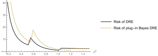
Figure 5. Risk function of the Bayes and plug–in DRE under log–Huber loss in normal models
p=N(0,σ2),q=N(1,σ2)and corresponding hyper–parametersξ=1,ξ=2=0,τ1=τ2=1, for all possible range ofσ2in Example1.
6. Concluding remarks
Estimating the ratio of two or more densities has received a widespread attention in recent years. Till date, most of the methods have been concentrated on solving this problem via nonparametric approaches. In this paper, we focused on a parametric Bayesian approach, when distributions come from the canonical form of the exponential family. We applied the log–Huber loss function to investigate the utility of the Bayesian and plug–in DRE . Our results confirm that Bayesian DRE along with the plug–in DRE (based on posterior expectations) perform similarly under log–Huber loss functions with the possibility of being exactly equal when the correction factorH=1. This is a somehow different result from a non–parametric point of view which is often the time the plug–in estimators perform poorly as opposed to empirical non–parametric Bayesian methods typically include stochastic processes such as the Gaussian process and the Dirichlet process. There are instances (for example, see Krnjajic et al. 2008, and the references therein) that for certain type of count data, the nonparametric Bayesian methodology provides enhanced flexibility to fit the data, provide rich posterior inferences, and provide finer predictive inference under a set of carefully selected criteria. However, there is an apparent major drawback. These processes have an infinite number of dimensions thus naive algorithmic approaches to computing posteriors is generally infeasible. Finally, the application to estimating theα–divergence between two PDF’s was discussed.
Acknowledgments:The authors thank Prof. Eric Marchand (Université de Sherbrooke) for his useful comments.
References
3. Ali, S. M. and Silvey, S. D. A general class of coefficients of divergence of one distribution from another.J.
Royal Stat. Soc. Ser. B1966,28, 131–142.
4. Berger, J.O.Statistical Decision Theory and Bayesian Analysis.New York, Springer- Verlag, 1985.
5. Csiszàr, I. Information-type measures of difference of probability distributions and indirect observation.
6. Deledalle, C. A. Estimation of Kullback-Leibler losses for noisy recovery problems within the exponential family.Electronic journal of statistics2017,11(2), 3141-3164.
7. Gretton, A., Smola, A., Huang, J., Schmittfull, M., Borgwardt, K., Schölkopf, B. Covariate shift by kernel mean matching. In J. Quiñonero-Candela, M. Sugiyama, A. Schwaighofer, N. Lawrence (Eds.), Data set shift in machine learning.Cambridge, MA, USA: MIT Press,Chapter 8, 131-160.
8. Hastie, T., Tibshirani, R., and Friedman, J.The Elements of Statistical Learning.Springer Series in Statistics. Springer New York Inc., New York, NY, USA, 2001.
9. Hido, S., Tsuboi, Y., Kashima, H., Sugiyama, M., Kanamori, T. Inlier-Based Outlier Detection via Direct Density Ratio Estimation.ICDM ’08 Proceedings of the 2008 Eighth IEEE International Conference on Data Mining
2008, 223-232.
10. Huber, P. Robust estimation of a location parameter,Annals of Mathematical Statistics196453, 73-101. 11. Kanamori, T., Hido, S., and Sugiyama, M. A Least-squares Approach to Direct Importance EstimationThe
Journal of Machine Learning Research2009,10, 1391-1445.
12. Krnjajic, M., Kottas, A., & Draper, D. Parametric and nonparametric Bayesian model specification: A case study involving models for count data.Computational Statistics & Data Analysis2008,52, 2110-2128. 13. Lehman, E.L. and Casella, G.Theory of point estimation. Springer Texts in Statistics.Springer-Verlag, New York,
second edition, 1998.
14. Murphy, Kevin P.Machine learning: a probabilistic perspective212,MIT press.
15. Nguyen, X., Wainwright, M.J., Jordan, M.I. Estimating divergence functional and the likelihood ratio by convex risk minimization.IEEE Transactions on Information Theory2010,56(11), 5847–5861
16. Póczos, B., Schneider, J. On the estimation of alpha-divergences.In Proceedings of the Fourteenth International
Conference on Artificial Intelligence and Statistics2011,609-617.
17. Nielsen F., Nock. "Entropies and cross–entropies of exponential families,"IEEE International Conference on
Image Processing, Hong Kong2010,3621-3624.
18. Quiñonero-Candela, J., Sugiyama, M., Schwaighofer, A., Lawrence, N.Dataset shift in machine learning.
Cambridge, MA, USA, MIT Press., 2009.
19. Shimodaira, H. Improving predictive inference under covariate shift by weighting the log-likelihood function.
Journal of Statistical Planning and Inference,902000,, 227-244.
20. Sugiyama, M., Yamada, M., Bunau, P.V., Suzuki, T., Kanamori, T., Kawanabe, M. Direct density-ratio estimation with dimensionality reduction via least-squares hetero-distributional subspace search.Neural
Networks, 242011,183-198.
21. Sugiyama, M., Kanamori, T., Suzuki, T., Hido, S., Sese, J., Takeuchi, I., and Wang, L. A density-ratio framework for statistical data processing. IPSJ Transactions on Computer Vision and Applications2009, 1, 183-208.
22. Sugiyama, M., Suzuki, T., Kanamori, T. Density ratio estimation in machine learning. Cambridge, UK, Cambridge University Press. 2012 a.
23. Sugiyama, Masashi and Kawanabe, Motoaki.Machine Learning in Non-Stationary Environments: Introduction
to Covariate Shift Adaptation.The MIT Press. 2012 b.
24. Sugiyama, M., Müller, K. R. Input-dependent estimation of generalization error under covariate shift.
Statistics and Decisions2005,23, 249-279.
25. Sugiyama, M., Krauledat, M., Müller, K. R.Covariate shift adaptation by importance weighted cross-validation.
Journal of Machine Learning Research,82007,985-1005.
26. Sugiyama, M., Suzuki, T., Nakajima, S., Kashima, H., von Bunau, P., and Kawanabe, M. Direct importance estimation for covariate shift adaptation.Annals of the Institute of Statistical Mathematics2008,60, 699-746. 27. Sugiyama, M. Hara, S. von Bünau, P. Suzuki, T. Kanamori, T. Kawanabe, M. Direct density ratio estimation
with dimensionality reduction.SIAM International Conference on Data Mining,. 2010.