Article
1
Agricultural land conversion, land economic value,
2
and sustainable agriculture: A case study from East
3
Java, Indonesia
4
Mohammad Rondhi1*, Pravitasari A. Pratiwi1, Vivi T. Handini1, Aryo F. Sunartomo2 and
5
Subhan A. Budiman3
6
1 Department of Agribusiness, Jember University; pravita.anjar@unej.ac.id, vivi.trisna@unej.ac.id
7
2 Department of Agricultural Extention, Jember University; aryo.faperta@unej.ac.id
8
3 Department of Soil Science, Jember University; sabudiman@unej.ac.id
9
* Correspondence: rondhi.faperta@unej.ac.id; Tel.: +6281291495040
10
11
Abstract: Agricultural land conversion (ALC) is an incentive–driven process. In this paper we
12
further investigate the inter–relationship between land economic value (LEV) and ALC. To achieve
13
this goal, we calculated LEV for agricultural and non-agricultural (housing) uses in two areas in
14
East Java, Indonesia. The first area represents suburban agriculture, facing rapid urbanization and
15
experiencing high rate of ALC. The second area represents rural agriculture with zero ALC.
16
Furthermore, we identified factors affecting LEV in both areas for both uses. The resut of this study
17
show that agricultural land yielded higher economic benefit in rural area. Conversely, comparing
18
to agricultural land, housing creates 7 times higher value in urban area. Moreover, agricultural
19
land shown to create higher profit after converted. Ironically, the similar comparison doesn’t exists
20
in rural area. Agricultural land only yielded 19% more value, indicate that agricultural land can be
21
easily converted. It is also proven by the growing number of new urban core in the periphery area.
22
There are several factors affecting land economic value, for agricultural use, soil fertility,
23
accessibility, and cropping pattern are important variables. While accessibility and location in
24
urban area increases land value for housing.
25
Keywords: Agricultural land conversion; land economic value; urbanization; land rent
26
27
1. Introduction
28
Land is one of the most important aspects of life. In agricultural production, the role of land as
29
the main input is irreplaceable. Economically, land is the most efficient wealth-generating asset for
30
farmer[1,2] and also an important factor for economic growth[3]. However, the limited and
31
unrenewable nature of land supply creates a fierce land–use competition, ussually between
32
agricultural and non–agricultural sector. This gives rise to agricultural land conversion (ALC) which
33
significantly reduces the agricultural land availability and threatens food supply. Irronically, the
34
highest rate of ALC occured in developing countries[4], which characterized by massive population
35
and high food consumption[5]. Thus a proper management of ALC is important for stabilizing food
36
supply.In addition to ALC, another important problem of agricultural land (AL) is the degradation
37
of land quality caused by unsuitable cropping pattern. In the effort to maximize economic gains,
38
farmer tend to overexploit land by cultivating high–value crop which basically unsuitable to land
39
characteristics. Although it produces a high economic return to farmer, in the longer term the land
40
qualitiy will be degraded and thus sacrificing the future food production for short–term economic
41
gains.
42
In Indonesia, the rate of ALC is 187,720 ha/yr and most of the converted land were used for
43
housing and industrial site development[6]. Housing development accounted for 48.96% of
44
converted land, followed by industrial (36.50%) and offices building development (14.55%) [7]. The
45
major causes of ALC in Indonesia is the low incentives received by farmers from agriculture [6]. The
46
rapid urban development in suburban area increases the value of AL for housing and thus gives
47
farmers higher incentive to convert their land. Morever, farmers often perceive selling their land as
48
an opportunity to find more promising job and as an effective way to earn quick cash and invest in
49
other sectors [6]. Hence, in 2009 the Indonesian governement issued a statute to protect and control
50
the rate of ALC under UU No. 41 Tahun 2009. The major mechanism proposed to control ALC is by
51
giving incentive to farmer for maintaining their agricultural activity. Specifically, the form of
52
incentives are decreasing land tax, improving agricultural infrastructure, funding research and
53
development of high yield variety, ease of access to agricultural information and technology,
54
providing farm input, securing land tenure, and rewarding farmer achievement [8]. The main
55
intention of this mechanism is to increase the economic value of agricultural activity. Since
56
increasing economic value of agriculture will lessen the likeliness of farmer to convert their land for
57
other use.
58
However, most of the proposed mechanisms are not inclusive for the majority of Indonesian
59
farmers. Consequently, the effort to increase economic value of agricultural activity is not effective.
60
Hence, it is important to reidentify factors which significantly affect land value to make this policy
61
efficient. Thus, the purpose of this paper is to identify factors affecting land value for agricultural
62
and housing–use. Spesifically, this paper compares land economic value in two distinct areas, rural
63
and suburban. Rural area is the representative of an agricultural economy while suburban area is the
64
representative of a transition economy from agricultural to industrial and service based economy.
65
The selection of rural and suburban area is important because both of those land are protected by
66
UU No. 41 Tahun 2009. The regulation protects agricultural land in both area to ensure food security,
67
since most of food in Indonesia produced in land–based agriculture, and most of these land located
68
in rural and suburban agricultural region.
69
Previous studies on land economic value shown that it significantly affect farmer decision to
70
sell or not to sell their land for non-agricultural purposes. In Europe, the Common Agricultural
71
Policy (CAP), through decoupled payments and environment schemes, increases land value because
72
farmers capitalize CAP payment into land value [9–12]. Those payments increase farmland value
73
and makes farmers unwilling to sell it. Furthermore, the increase in farmland value promote a land
74
use conflicts both between farmers (for agricultural use) and between farmers and non-farmer (for
75
non-agricultural uses)[13]. Moreover, increasing land economic value due to urbanization in
76
Bangladesh makes real estate and individual developer speculate and develop building in restricted
77
area including in productive agricultural land [14]. In Indonesia, the rapid urbanization increases
78
demand for housing resulting in high demand for land for housing development, thus increases the
79
value of agricultural land for non-agricultural use. The increasing land economic value for housing
80
translated into massive ALC and creates an area called suburban agriculture [15]. These studies
81
show that land economic value is the main driver of ALC, however very little study stresses mainly
82
on this issue and thus proposing less focused policy implications.
83
The main contribution of this paper is that it demonstrates that ALC is driven by differing land
84
economic value (land economic value for agricultural use is lower comparing to other uses). Slightly
85
different from the previous findings which stated that ALC is driven by external factors (e.g.
86
government policies, industrialization, urbanization, etc) or internal factors (e.g. soil structure,
87
fertility, etc), this paper stresses that both external or internal factors may promote or prevent ALC
88
depended on whether they increase or decrese land economic value for agricultural use. If they
89
increase land economic value for agricultural use they will prevent ALC and conversely, they will
90
promote ALC if they decrease land economic value for agricultural use whether it is intentionally or
91
not. The important point is that the effort to prevent ALC will be effective if it focused on increasing
92
land economic value for agricultural use. Thus, the other contribution of this paper is by identifying
93
factors affecting land economic value both for agricultural and non-agricultural use.
94
The rest of the paper is structured as follows; the next section (Material and Methods) describes
95
study area, data and sampling design, and analytical procedure. The third section (Results)contains
the findings of our study. The fourth section (Discussions) discusses our finding in the context of
97
previous literature. Finally, the last section (Conclusion) concludes our findings, states policy
98
implications and mentions future research needs.
99
2. Materials and Methods
100
2.1. Study Area
101
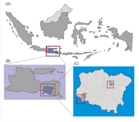
This study was conducted at two different villages in Jember District (Kabupaten) which is
102
located in the Province of East Java (Figure 1). Jember is the typical agricultural region in Indonesia.
103
From a total of 3293.34 square kilometer of land, agriculture accounts for 50.1% of total land use. In
104
Indonesia, the agricultural production concentrated in the island of Java and East Java being one of
105
the main agricultural regions. In East Java, rice production mainly concentrated in Jember. However,
106
Jember’s economy is experiencing a structural transformation from agricultural to industrial and
107
service based economy. Consequently, the rate oof ALC in Jember is increasing in the past decade.
108
109
Figure 1 Map of study area, (A) Province of East Java relative to Indonesia, (B) Jember District
110
relative to Province of East Java, (C) Gumukmas (lower) and Sumbersari (upper) Subdistrict.
111
Between 2009 and 2016, the annual rate of ALC in Jember was 70.77 hectare (0.085%). Most of
112
the converted land were used for housing and industrial development. From 31 subdistricts, ALC
113
occured only in 9 subdistricts, with highest ALC is 8.6036% and the lowest is 0.7687% [16]. However,
114
the pattern of ALC shows some important information. There are 22 subdistricts which do not
115
experienced ALC, however the rate of agricultural growth is zero. It means that there will be
continuing ALC in the next few years. Moreover, Jember municipality area consisted of 3
117
subdistricts in which the rate of ALC are high, the fact that there 6 others subdistricts which
118
experienced ALC show that there are new urban core. Furthermore, this new urban core were
119
previously an agricultural region. Thus it is important to study land economic value in urban and
120
rural region.
121
The first village was Kepanjen and located in Gumukmas Subdistrict (Kecamatan). Kepanjen is
122
the representative of agricultural economy. Kepanjen has experienced zero ALC during 2009–2016
123
and the main crop planted are horticulture and food crop (Figure 2). Kepanjen has an area of 14.78
124
square kilometer and a population of 10,515 inhabitants, resulting in a population density of 711
125
person/square kilometer.
126
127
Figure 1 Map of Kepanjen Village, (A) Land use distribution in 2012, (B) Land use distribution in
128
2017 showing a relatively constant agricultural land and housing.
129
The second village was Antirogo which located in Sumbersari Subdistrict. Antirogo is the
130
representative of suburban agricultural area. It located 7 km from Jember downtown and has
131
experienced rapid ALC of 8.6% during 2009–2016 (Figure 3). The average rate of ALC in Jember
132
during 2009–2016 was 0.085%, it shows that ALC is concentrated in the suburban area. Antirogo was
133
located 7 km away from Jember dowtown and has population density of 1359 person/square
134
kilometer. The selection of these villages based on practical reason, both villages are agricultural
135
based region, where Kepanjen continue to remain in agriculture while Antirogo demonstrates a
136
significant shift in their economic structure to a more industrialized economy. Both farmer and
137
home–owner in both villages were selected as respondents of this study.
The sampling procedure used was multi–stage random sampling. In the first stage the
139
population of farmer and home–owner in both villages were enumerated. In the first stage we have
140
identified 6061 home–owners (3011 in Kepanjen and 3050 in Antirogo) and 1839 farmers (783 in
141
Kepanjen and 1056 in Antirogo). In the second stage we randomly selected 50 farmers and 50
142
home–owners in each village, resulting in total 200 respondents.
143
144
Figure 3 Map of Antirogo Village, (A) Land use distribution in 2012, (B) Land use distribution in
145
2017, showing a growing land for housing.
146
2.2. Data
147
The data used in this study were collected from 100 farmers and 100 home–owners from each
148
villages. The survey was performed between January and June 2018. The survey has two parts, the
149
first part focused on measuring land economic value both for agricultural and housing use while the
150
second part focused on eliciting farmer and home–owner characteristics.
151
We measured land economic value as the economic rent it produced for a period of one year.
152
Economic rent for agricultural land calculated as profit obtained from farm production in a year.
153
Similarly, economic rent of housing calculated as the amount of rental fee obtained by home–owner
154
from leasing their house for a period of one year after deducted by house operational and
155
maintenace costs.
156
There are eight variables used to explain farmland characteristics namely, land basic
157
information (land area, land tenure, location), accessibility (distance to irrigation, distance to nearest
158
market, and distance to road), cropping pattern and soil fertility. Cropping pattern in both villages
159
varied, there are 10 patterns in Kepanjen and two in Antirogo. Cropping pattern in Kepanjen are
160
mostly food and horticultural crops and food and seasonal plantation crop in Antirogo. All of these
161
pattern grouped into food crops (dummy value 0) and mixed crops (dummy value 1). Soil fertility
162
determined by directly asking farmer knowledge about their land. The use of self–reported soil
163
fertility level has been found useful since soil fertility level is commonly know by farmer. Soil
164
fertility were grouped into fertil land (1) and less fertile land (0).
165
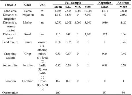
The descriptions of farmland data used in this study—full sample, rural and urban area—are
166
shown in Table 1. Although the average differs slighly, rural farmer has wider land possession than
167
their counterpart. It is also shown that agricultural land has easier access to irigation with only 42 m
168
in average, comparing to land in urban area which located 2,053 m away from in average. Both
distance to nearest market and to road tend to not significantly different, as many farmers both in
170
rural and urban area tend to sell their harvest to collecting trader directly at their plot. Most of land
171
are owned by farmer, 88 percent farmers in both villages cultivate their own land. However, most of
172
them cultivate only food crops all year long, only 33 percent farmers doing mixed cultivation. In
173
realtion to soil fertility, most farmers (82 percent) regarded their land as fertil.
174
Table 1. Descriptive statistics for farmland.
175
Variable Code Unit Full Sample Kepanjen Antirogo
Mean S.D. Min. Max. Mean Mean Land area L.area m2 4,005 2,515 1,000 10,000 4,211 3,800
Distance to irrigation
Irrigation m 1,047 1,681 0 5,000 42 2,053
Distance to nearest market
Market m 4,250 1,305 2,000 8,000 4080 4420
Distance to road
Road m 113 147 1 1,000 123 104
Land tenure Tenure owner (1), other(0)
0.88 0.32 0 1 1 0.76
Cropping pattern
Crop mixed (1), food
(0)
0.33 0.47 0 1 0.26 0.40
Soil fertility Fertility fertile (1), less
fertile (0)
0.82 0.38 0 1 0.88 0.76
Location Location Urban (1), rural
(0)
0.5 0.5 0 1 0 1
Observation 100 50 50
There are six variables used to describe housing conditions in both villages. Information
176
regarding housing land characteristics are summarized in Table 2.
177
Table 2. Descriptive statistics for housing characteristics.
178
Variable Code Unit Full Sample Kepanjen Antirogo
Mean S.D. Min. Max. Mean Mean
Building area B.area m2 71 26 27 198 74 68
No. of room Room m 3 1 2 8 3 3
Distance to road
Road m 117 170 1 1,000 184 50
Distance to downtown
Downtown m 6,135 1,670 3,500 10,000 6350 5920
Water availability
Water sufficient(1), insufficient(0)
0.95 0.26 0 1 1 0.94
Location Location Urban (1), rural (0)
0.5 0.5 0 1 1 0
Observation 100 50 50
Both urban and rural house has 3 rooms in average, like typical house in Indonesia. The slight
179
difference exists in water availability, 100 percent rural houses have sufficient water, meanwhile
there 4 percent houses in urban area which do not have access to sufficient water. It shows that
181
urban development not only resulting in agricultural land conversion but also started to degrade
182
water quality. Urban area has easier access both to road and to downtown area, since both of this
183
infrastructures are the result of economic development.
184
2.3. Econometric Model and Estimation Procedures
185
As previously mentioned, we calculated land economic value as the rent created by that land
186
when used for agricultural or housing purposes. The economic rent created from agricultural land
187
calculated by Equation 1.
188
(
it it)
it ata
q
p
c
l
L
×
−
=
(1)Where
l
at is agricultural land rent for year t,q
it is quantity harvested at season i on year t,p
it is189
the price of harvested crop at season i on year t,
c
it is the total farming cost at season i on year t,190
while
L
a is land area. While economic rent created from housing is calculated by Equation 2.191
[
t t]
ht
h
R
c
l
L
−
=
(2)Where
l
ht is economic rent from housing at year t,R
t is the rental fee of house for year t,c
t is192
house operational and maintenance cost for year t, while
L
h is the house building area.193
After calculating land economic value we then determine factors affecting it. We employed
194
multiple linear regression. There two equations estimated in this stage. The first equation is
195
attempted to determine factors affecting land economic value both in rural and urban area (Equation
196
3).
197
0
1 1
n m
ai n in m im i
n m
l
α
α
x
β
D
u
= =
=
+
+
+
(3)Where
i
=
1...100
,l
ai is agricultural land value,x
n is quantitative variables,D
m is qualitative198
variables, and
α α α
0,
n,
m are regression intercept, coefficients for quantitative and qualitative199
variables respectively. The description of each variable and their summary statistics are shown in
200
Table 1. The second equation were used to estimate factors affecting land economic value for
201
housing and shown in Equation 4.
202
0
1 1
n m
hi n in m im i
n m
l
α
α
x
β
D
u
= =
=
+
+
+
(4)Where
i
=
1...100
,l
hi is land economic value for housing,x
n is quantitative variables,D
m is203
qualitative variables, and
α α α
0,
n,
m are regression intercept, coefficients for quantitative and204
qualitative variables respectively. The description of each variable and their summary statistics are
205
shown in Table 2. The data used in this study has been tested for autocorrelation, heteroscedasticity,
206
and multicollinearity. The estimation of these equation were based on ordinary least square
207
estimation and the estimation processes were conducted with SPSS Software (version 25; SPSS Inc.,
208
Chicago, IL, USA)
3. Results
211
3.1. Land Economic Value
212
Land rent analysis revealed that urban area has lower value for agriculture but higher value for
213
housing (Table 3). The average agricultural land value in urban area is Rp 4,447/m2/year ranging
214
between Rp −416/m2/year and Rp 10,975/m2/year. Meanwhile, in rural area it averaged at Rp
215
6,047/m2/year ranging between Rp 1,600/m2/year and Rp 19,504/m2/year. Conversely, the average
216
housing land value in urban area is Rp 39,904/m2/year with a wide range of Rp 7,917/m2/year and Rp
217
142,188/m2/year, it is 7 times higher in average comparing to the conditions in rural area. In rural
218
area, housing value only averaged at Rp 5,059/m2/year ranging between Rp 278/m2/year and Rp
219
14,908/m2/year. There is a negative value in urban agriculture, it means that there is farmers who
220
choose to remain in farmland even at the expense of farming profits. While urban housing yielded 7
221
times higher value, the similar condition doesnt exists in rural agriculture where agricultural land
222
yielded only 19% higher value.
223
Table 3. Land economic value for agricultural and housing purpose in the study area
224
Land use Unit Rural Area Urban Area Full Sample
Mean Min. Max. Mean Min. Max. Mean
Agriculture Rp/m2/year 6,047 1,600 19,504 4,447 −416 10,975 4,997
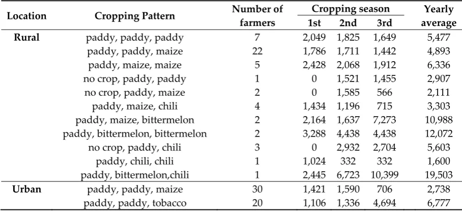
Housing Rp/m2/year 5,059 278 14,908 39,954 7,917 142,188 22,312
Although most farmers cultivating food crops all year long, we found various cropping pattern
225
and each cropping pattern has different economic value (Table 4). In rural area, non food crop
226
pattern are mixed with horticular crops, while in urban area non food crop pattern only mixed with
227
seasonal plantation crop which is tobacco. The land value reveal that non food cropping pattern
228
yielded higher value. However, only 26 percent farmers in rural area and 40 percent in urban area
229
who cultivated non food crops. Both horticultural and seasonal plantation crops require high
230
farming costs and also have greater production and price risks. Thus only wealthier farmers who
231
able to bear greater farming costs and risks. On the other hand, the growing number of commercial
232
farmer in rural area who cultivated horticultural crops are bringing potential problem. Motivated by
233
high economic gains, they tend to overexploite land by cultivating horticultural crops which
234
basically unsuitable to land characteristics. Although generated high value, this practices will
235
degrade soil quality in the long term.
236
Table 4. Land economic value of agricultural land under different cropping pattern
237
Location Cropping Pattern Number of
farmers
Cropping season Yearly average 1st 2nd 3rd
Rural paddy, paddy, paddy 7 2,049 1,825 1,649 5,477
paddy, paddy, maize 22 1,786 1,711 1,442 4,893
paddy, maize, maize 5 2,428 2,068 1,912 6,336
no crop, paddy, paddy 1 0 1,521 1,455 2,907
no crop, paddy, maize 2 0 1,585 566 2,111
paddy, maize, chili 4 1,434 1,196 715 3,303
paddy, maize, bittermelon 2 2,164 1,637 7,273 10,988 paddy, bittermelon, bittermelon 2 3,288 4,438 4,438 12,072
no crop, paddy, chili 3 0 2,932 2,704 5,603
paddy, chili, chili 1 1,024 332 332 1,600
paddy, bittermelon,chili 1 2,445 6,723 10,399 19,503
Urban paddy, paddy, maize 30 1,421 1,590 706 2,738
In rural area, the houses are located only in land previously intended for housing purpose.
238
Conversely, there are houses built in converted land previously used for agricultural production.
239
The result of analysis reveal that agricultural land yielded higher economic value after converted
240
(Table 5). In average converted agricultural land yielded Rp. 7,917/m2/year ranging between Rp.
241
7,917/m2/year and Rp. 42,230/m2/year. It is significantly higher than when it was retained as
242
agricultural land. Thus, it is logical for farmer to convert their land since it give higher benefit than
243
remaining in agriculture.
244
Table 5. Land economic value for converted agricultural land
245
Land origin Economic value (Rp/m
2/year)
Mean Minimum Maximum
Converted agricultural land 7,917 7,917 42,230
Housing 45,063 45,063 142,188
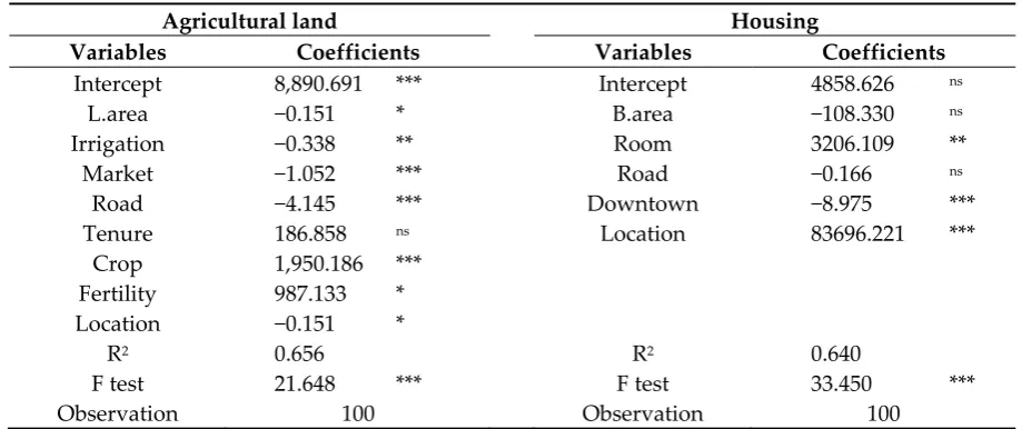
3.2. Factors Affecting Land Economic Value
246
Ordinary least square estimation revelead that many variables affect economic value of land
247
used for agricultural and non agricultural purposes. Table 6 presents estimation results of Equation
248
(3) and (4). The F test for the overall fit of both model are shown in Table 4. It tests the null
249
hypothesis that all coefficients in the models are 0. Since the F test p value for both models are p <
250
0.05; p = 0.000, the null hypothesis that all variables coefficients are 0 is rejected. Thus, it can be
251
concluded that the model is better at estimating land economic value for both agricultural and
252
housing use. The explained variance of dependent variable can be measured with R2 value. The R2
253
value of the first model is 0.656 indicates that 65.6% of agricultural land value variation can be
254
explained by the model. The R2 value of the second model is 0.640 indicates that 64% of housing land
255
value variation can be explained by the model.This percentage is satisfactory since the models didn't
256
violate the normality, multicollinearity, homoscedasticity and linearity assumptions.
257
Table 6. Estimation results
258
Agricultural land Housing
Variables Coefficients Variables Coefficients
Intercept 8,890.691 *** Intercept 4858.626 ns
L.area −0.151 * B.area −108.330 ns
Irrigation −0.338 ** Room 3206.109 **
Market −1.052 *** Road −0.166 ns
Road −4.145 *** Downtown −8.975 ***
Tenure 186.858 ns Location 83696.221 ***
Crop 1,950.186 ***
Fertility 987.133 *
Location −0.151 *
R2 0.656 R2 0.640
F test 21.648 *** F test 33.450 ***
Observation 100 Observation 100
note, ***= p<0.01, ** = 0.01>p>0.05, * = 0.05>p>0.1, ns = p>0.1
259
The first model shows that 7 out of 8 variables estimated have significant p values. As expected
260
land area has a negative coefficient, thus the larger the land the lower its economic value. Since a
261
larger land will require largest farming cost, promoting cost–minimizing behaviour, resulting in
262
lower productivity. Accessibility variables provide result as expected, the further the farmland from
263
irrigation, nearest market, and road the lower land value is. Although much of the selling of
264
harvested crop occured in farmland, the seller ussually charges larger transportation cost. Cropping
265
pattern significantly affect land value, where non food crops in average generated Rp
1,950.186/m2/year higher value comparing to food crops pattern. Soil fertility also reported to
267
increases land economic value by Rp 987.133/m2/year in average. Furthermore, as expected,
268
farmland located in urban area generated less value comparing to those in rural area. However, land
269
tenure doesnt significantly affect land value. The explanation for this result is that all farmers from
270
rural area cultivated their own land, resulting in little variation in the data.
271
The second model shows that 3 out of 5 variables estimated have significant effect to housing
272
land value. Number of room and accesibility to downtown area shown to be significantly affect land
273
value. Most house renter in studied area prefer the number of room than the size of building, since
274
most of them rented house in group. Thus, the greater the number of room the greater economic
275
value it generated. Furthermore, people in prefer nearest location to downtown area since most of
276
their activity conducted there. Furthermore, as expected, house located in urban area generates Rp
277
83696.221/m2/year higher value comparing to those located in rural area.
278
4. Discussion
279
4.1. Land Economic Value and Agricultural Land Conversion
280
The main purpose of this study was to calculate land economic value in rural and suburban
281
area. The point of conducting this study in these areas was to compare land economic value in an
282
area with zero ALC (rural) and area with high ALC (suburban). Our result demonstrates that there is
283
a significant different in land economic value in these areas. In rural area, land creates more value
284
when used for agricultural purposes. While in urban area, it creates higher value when used for
285
housing purpose. However, although creating higher value, agricultural production has only 19%
286
higher value comparing to housing use. Significantly different with the condition in urban area,
287
where housing use has 790% higher value.This significant difference indicates that there is a strong
288
pressure for agricultural land in suburban area. Furthermore, it also indicates how likely the land
289
use will evolve in the future. It suggests that ALC rate in suburban area will continue to increase and
290
remove agricultural use completely as has happened in Italy (See Table 3 and 5) [17].
291
Previous studies oftenly relate ALC to rapid urbanization and economic development in urban
292
area [18–22]. A common view is that urbanization means more people living in the urban area,
293
increasing the demand of land for housing. As a plain land, agricultural land has always been
294
converted to meet this demand. The suburban area in our study demonstrates a similar conditions.
295
As Jember economy continue to growth and transform into an industrial and service based industry,
296
it promotes rapid urbanization. However, the benefits rendered by this growth yielded a negative
297
impacts, specifically to farmers. Farmers oftenly converted their land because of incentive received
298
from agricultural sector is much less than in other sector. Moreover, high land price for housing
299
motivate farmer to sell it for cash. Although farmers receive high compensation from selling land,
300
they are actually facing difficulty in managing it for investments [23]. In addition, although currently
301
rural area record zero ALC, the narrow difference in land economic value indicates that ALC can be
302
happen anytime in the future. Since farmers tend to not willing to sell their land only when they
303
receive high economic value from it [9,10,10–12].
304
4.2. Factors Affecting Land Economic Value
305
The next result of our study on factors affecting land economic value supports the findings of
306
previous studies. We found that land area decrease land value both for agricultural and housing use.
307
This result is in line with the finding of [24–28], the economic value decrease with the increase in
308
land area. Both wider agricultural or housing use require higher input and cost, thus offsetting the
309
revenue. Furthermore, in urban area, farmer with more land tend to use family labor to minimize
310
labor cost, this resulted in lower productivity. While in rural area, farmer with more land tend to
311
cultivate low risk low revenue crop such as rice and maize. Conversely, farmer with smaller land
312
tend to maximize their income by cultivating high value crop such as horticultural crop. While for
313
housing, larger house require higher maintenance cost. In addition, the demand for larger house is
not as high as demand for smaller house since the house tenants tend to be a small family who prefer
315
lower rental cost than large sized house.
316
The accessibility variables (distance to irrigation, to nearest market, and to road) show negative
317
effect. This result is in line with the results from [27–30]. Distance to market tend to put a negative
318
effect on land value [31–34]. Similarly, distance to irrigation and to road has a negative impact on
319
land value [35–37]. Specifically, irrigation at the study area required greater fee for plots located far
320
from irrigation canals. Similarly, distance to road increase the transportation cost of farm production
321
as well as increasing the difficulty of access.
322
323
Figure 4 Horticultural and seasonal plantation crops, (A) Cayenne pepper in Kepanjen, (B) Dragon
324
fruit in Kepanjen, (C) Tobacco in Antirogo, (D) Bittermelon in Kepanjen, (E) Water melon in
325
Kepanjen, (F) Chili in Kepanjen
326
This study identified three cropping seasons annually and most farmers apply crop rotation,
327
only 1% of farmers do not apply crop rotation. Crop rotation found to be positively affect land value,
328
which means that land cultivated with various types of crops in one year (horticulture or
plantations, see Figure 4) has higher economic value those cultivating only food crops. The
330
difference in types of crops significantly affects land value, because it is directly related to the output
331
produced as well as the price of output [32,38]. We found more cropping pattern in Kepanjen than in
332
Antirogo. Land suitability is the major cause of this difference, Kepanjen has more crops suitable for
333
a variety of cropping. Furthermore, more farmer in Kepanjen tend to maximize their farm income by
334
cultivating high–value crops. Variable closely related to cropping pattern is land fertility. Measured
335
based on farmer knowledge, land fertility has positive effect on land value, just as has been shown
336
by previous studies [25,32,36,38,39]. Moreover, agricultural land in rural area tend to be more fertile
337
than those in the urban area.
338
Location dummy (whether the plots located in urban or rural area) also has positive impact on
339
land value. The previous result presented that agricultural land in rural area has higher value. To
340
find out whether it is true that location of agricultural land will statistically affect land value,
341
location was entered as a dummy variable. The results show that statistically, location significantly
342
influence land value. The negative sign strengthens the results that the agricultural land in rural has
343
higher value. This result is different from the study of [32] and [25] which stated that agricultural
344
land close to downtown Buenos Aries and Walles is of higher value. This is caused by the difference
345
characteristics of land located in urban and rural areas. These characteristics are cultivated plants..
346
Horticultural commodities cultivated in rural area have high selling value, moreover, the land in this
347
area are fertile (90% of the respondents stated the land in the fertile region), this causes higher
348
income. While agricultural land in urban area according to 24% of the farmers are infertile, even
349
though they planted with tobacco, the yield per unit of land is not too high.
350
4.3. Policy Implications
351
Finally, although this study was conducted at the village level, the result can be generalized to
352
the conditions of other area. The similarity of results with the findings of previous studies in all over
353
the world show that this study can be generalized to the extent of the generated result. There is a
354
strong basis to support the hypothesis that ALC is driven by the significant difference in land
355
economic value for different purpose. We predict that in the future ALC in urban area will continue
356
to increase since the the demand for housing is not showing any sign of decrease. In addition, we
357
stated that in rural area, although currently experiencing zero ALC and also agricultural production
358
playing a central economic role, there is a possibility that ALC will occur in the future. The slight
359
difference in land value in rural area shows that the resistance to convert agricultural land to non
360
agricultural use is weak.
361
However, there are two exceptions to this. First, in urban area, the minimum value for
362
agricultural land has negative sign. It means that there are farmers who choose to preserve their land
363
even at the expense of profit. As shown by [40] that there are a growing number of farmers who
364
choose to remain in farming and do not participate in land speculation and real estate market (urban
365
farmer). The importance point of this farmers is that they tend to retain their farmland and thus
366
preventing ALC. A systematic identification of this farmers and a targeted incentive for their
367
farming activity will surely increase their motivation in farming. Second, in rural area, although the
368
economic value generated by farming is only a little higher than housing use, farmer started to
369
cultivate high value crop. It shows that there is a shift of motive in farming at rural area from
370
subsistence to commercial farming. If the number of commercial farmer increase, the possibility of
371
ALC in rural area will be significantly low.
372
In the context of Indonesian National Policy, agricultural sector faces a difficult problem in
373
relation to ALC. As a developing contries, Indonesian economic and demographic structure
374
experiencing rapid transformation into a more industrialized and modern society. Consequently, the
375
need for land whether for housing or industrial purpose is high. On the other hand, there is strong
376
need to preserve agricultural land to support food security. Thus, preventing ALC and preserving
377
agricultural land require a properly planned policy. Based on the result of this study we suggest
378
three options that can be used to control ALC in rural and urban area in the farmework of land
379
economic value.
1. The current incentive mechanism contained in UU No. 41 Tahun 2009 should be focused on
381
farmer in urban area, specifically to those who choose to remain in farming even at the expense
382
of profit (urban farmer). Since the current incentive mechanism require proactive and highly
383
motivated farmer.
384
2. There should be an effort to encourage farmer to cultivate crop which is suitable to land
385
characteristics. Although cultivating high value crop actually increase land value, however,
386
land quality (fertility) will be degraded if the land is forced to produce crop which is basically
387
unsuitable to its characteristics [41,42]. This is one of the major causes of land quality
388
degradation. Since land fertility is proven to be positively affect land value both theoretically
389
and empirically, uncontrolled land quality degradation will sacrifice the sustainability of
390
agriculture itself. Thus, it is important to conduct a detailed analysis on land suitability for
391
cropping pattern especially in rural area. This should be a main agenda in the framework of
392
increasing agricultural land economic value in rural area.
393
3. The growing number of commercial farmer in rural area should be supported with access to
394
timely information regarding market conditions and farm technology. Commercial farmer tend
395
to be more responsive to new information and technology. Thus, improving their access to
396
technology will further improve their farming productivity [43,44].
397
5. Conclusions
398
This study attempted to measure the economic value of land in rural and urban area both for
399
agricultural and non–agricultural use. The main thesis of this study is that land value is the main
400
driver of agricultural land conversion. The higher the value of agricultural land for agricultural use
401
will prevent land conversion and vice versa. The result of this study support the previous thesis. In
402
urban area where the demand for housing is high, land value for housing use increases rapidly, thus
403
promoting agricultural land conversion. While in rural area, where agriculture is the main economic
404
activity, agricultural land has higher value. We also found the emergence of urban farmer who
405
choose to remain in farming and retain their farmland even at the expense of profit. In rural area,
406
there is a growing number of commercial farmer who easily rotate their cultivated crop with high
407
value one, although receiving high economic return, they tend to neglect land suitability resulting in
408
the potential degradation of land quality.
409
Finally, we propose further research direction based on the result of this study. This research
410
direction will provide information in an effort to increase land economic value for agricultural use to
411
prevent and control ALC. The required further research are,
412
• It is required to systematically identify the characteristics of urban farmer and explore
413
thoroughly what motivate them to remain in farming and retain their farmland.
414
• It is needed also to identify the characteristics of commercial farmer in rural area and trace how
415
they acquire information regarding market conditions and technology that they used in making
416
farm decision.
417
• Finally, it is important to identify agricultural land suitability analysis and measure the
418
economic benefit to cultivate crop which suitable with land characteristics.
419
Author Contributions: Conceptualization, Mohammad Rondhi, Pravita Pratiwi, Vivi Handini, Aryo
420
Sunartomo and Subhan Budiman; Data curation, Mohammad Rondhi, Pravita Pratiwi, Vivi Handini, Aryo
421
Sunartomo and Subhan Budiman; Formal analysis, Mohammad Rondhi, Pravita Pratiwi, Vivi Handini, Aryo
422
Sunartomo and Subhan Budiman; Funding acquisition, Mohammad Rondhi, Aryo Sunartomo and Subhan
423
Budiman; Methodology, Mohammad Rondhi, Pravita Pratiwi, Vivi Handini and Subhan Budiman; Project
424
administration, Mohammad Rondhi, Aryo Sunartomo and Subhan Budiman; Supervision, Mohammad Rondhi;
425
Visualization, Subhan Budiman; Writing – original draft, Mohammad Rondhi, Pravita Pratiwi, Vivi Handini,
426
Aryo Sunartomo and Subhan Budiman..
427
Funding: This research was funded by Regional Development Planning Agency (BAPPEDA) Jember, grant
428
number 074/339.1/310/2017.
429
Acknowledgments: In this section we wish to acknowledge the helpful cooperation of farmers and
430
home–owners interviewed in this study. We also feel thankful to Regional Government of Jember and Jember
University for supporting this study. Personally we wish to acknowledge the helpful contribution of Yoga
432
Satria Siaga in the preparation of this manuscript. Finally, all errors are ours.
433
Conflicts of Interest: The authors declare no conflict of interest.
434
References
435
1. Sitko, N. J.; Jayne, T. S. Structural transformation or elite land capture ? The growth of ‘“ emergent ”’
436
farmers in Zambia. Food Policy2014, 48, 194–202, doi:10.1016/j.foodpol.2014.05.006.
437
2. Muyanga, M.; Jayne, T. S.; Burke, W. J. Pathways into and out of Poverty : A Study of Rural Household
438
Wealth Dynamics in Kenya. J. Dev. Stud.2013, 49, 37–41, doi:10.1080/00220388.2013.812197.
439
3. Li, J. Land sale venue and economic growth path : Evidence from China ’ s urban land market. Habitat
440
Int.2014, 41, 307–313, doi:10.1016/j.habitatint.2013.10.001.
441
4. Azadi, H.; Ho, P.; Hasfiati, L. Agricultural land conversion drivers: A comparison between less
442
developed, developing and developed countries. L. Degrad. Dev.2011, 22, 596–604, doi:10.1002/ldr.1037.
443
5. Deloitte The food value chain A challenge for the next century; London, 2013;
444
6. Agus, F.; Irawan Agricultural Land Conversion As A Threat to Food Security and Environtmental
445
Quality. J. Litbang Pertan.2006, 25, 90–98.
446
7. Irawan, B. Meningkatkan Efektivitas Kebijakan Konversi Lahan. Forum Penelit. Agro Ekon. 2008, 26,
447
116–131.
448
8. Government of Indonesia Perlindungan Lahan Pertanian Berkelanjutan; Indonesia, 2009; p. 24;.
449
9. Kilian, S.; Antón, J.; Salhofer, K.; Röder, N. Impacts of 2003 CAP reform on land rental prices and
450
capitalzation. Land use policy2012, 29, 789–797, doi:10.1016/j.landusepol.2011.12.004.
451
10. Latruffe, L.; Le Mouël, C. Capitalization of government support in agricultural land prices: What do we
452
know? J. Econ. Surv.2009, 23, 659–691, doi:10.1111/j.1467-6419.2009.00575.x.
453
11. Feichtinger, P.; Salhofer, K. What do we know about the influence of agricultural support on
454
agricultural land prices? A summary of results. In Land, Labour And Capital Markets in European
455
Agriculture: Diversity Under A Common Policy; Swinnen, J., Knops, L., Eds.; Centre For European Policy
456
Studies (CEPS): Brussels, 2013; pp. 14–27.
457
12. Ciaian, P.; Kancs, D.; Swinnen, J. The Impact of Decoupled Payments on Land Prices in the EU. In Land,
458
Labour And Capital Markets in European Agriculture: Diversity Under A Common Policy; Swinnen, J., Knops,
459
L., Eds.; Centre For European Policy Studies (CEPS): Brussels, 2013; pp. 28–42.
460
13. Milczarek-Andrzejewska, D.; Zawalińska, K.; Czarnecki, A. Land-use conflicts and the Common
461
Agricultural Policy: Evidence from Poland. Land use policy 2018, 73, 423–433,
462
doi:10.1016/j.landusepol.2018.02.016.
463
14. Alam, M. J. Rapid urbanization and changing land values in mega cities: implications for housing
464
development projects in Dhaka, Bangladesh. Bandung J. Glob. South 2018, 5, 2,
465
doi:10.1186/s40728-018-0046-0.
466
15. Pribadi, D. O.; Pauleit, S. The dynamics of peri-urban agriculture during rapid urbanization of
467
Jabodetabek Metropolitan Area. Land use policy2015, 48, 13–24, doi:10.1016/j.landusepol.2015.05.009.
468
16. BPS-Statistics of Jember Regency Jember Regency in Figures; BPS Kabupaten Jember: Jember, 2017;
469
17. Manganelli, B.; Murgante, B. The Dynamics of Urban Land Rent in Italian Regional Capital Cities. Land
470
2017, 6, 54, doi:10.3390/land6030054.
471
18. Peerzado, M. B.; Magsi, H.; Sheikh, M. J. Land use conflicts and urban sprawl: Conversion of agriculture
472
lands into urbanization in Hyderabad, Pakistan. J. Saudi Soc. Agric. Sci. 2018,
473
doi:10.1016/j.jssas.2018.02.002.
19. Kontgis, C.; Schneider, A.; Fox, J.; Saksena, S.; Spencer, J. H.; Castrence, M. Monitoring
475
peri-urbanization in the greater Ho Chi Minh City metropolitan area. Appl. Geogr.2014, 53, 377–388,
476
doi:10.1016/j.apgeog.2014.06.029.
477
20. Wasilewski, A.; Krukowski, K. Land conversion for suburban housing: A study of urbanization around
478
Warsaw and Olsztyn, Poland. Environ. Manage.2004, 34, 291–303, doi:10.1007/s00267-003-3010-x.
479
21. Phuc, N. Q.; Westen, A. C. M. va.; Zoomers, A. Agricultural land for urban development: The process of
480
land conversion in Central Vietnam. Habitat Int.2014, 41, 1–7, doi:10.1016/j.habitatint.2013.06.004.
481
22. Xiao, R.; Liu, Y.; Huang, X.; Shi, R.; Yu, W.; Zhang, T. Exploring the driving forces of farmland loss
482
under rapidurbanization using binary logistic regression and spatial regression: A case study of
483
Shanghai and Hangzhou Bay. Ecol. Indic.2018, 95, 455–467, doi:10.1016/j.ecolind.2018.07.057.
484
23. Nguyen, T. H. T.; Tran, V. T.; Bui, Q. T.; Man, Q. H.; Walter, T. de V. Socio-economic effects of
485
agricultural land conversion for urban development : Case study of Hanoi , Vietnam. Land use policy
486
2016, 54, 583–592, doi:10.1016/j.landusepol.2016.02.032.
487
24. Brown, K.; Barrows, R. The impact of soil conservation investments on land prices. Am. J. Agric. Econ.
488
1985, 67, 943–947.
489
25. Maddison, D. A hedonic analysis of agricultural land prices in England and Wales. Eur. Rev. Agric. Econ.
490
2000, 27, 519–532, doi:DOI 10.1093/erae/27.4.519.
491
26. Maddison, D. J. A spatio-temporal model of farmland values. J. Agric. Econ. 2009, 60, 171–189,
492
doi:10.1111/j.1477-9552.2008.00182.x.
493
27. Troncoso, J. L.; Aguirre, M.; Manriquez, P.; Labarra, V.; Ormazábal, Y. Influence of physical attributes
494
on the price of land: the case of the Province of Talca, Chile. Cienc. e Investig. Agrar.2010, 37, 105–112,
495
doi:10.4067/S0718-16202010000300009.
496
28. Yoo, J.; Simonit, S.; Connors, J. P.; Maliszewski, P. J.; Kinzig, A. P.; Perrings, C. The value of agricultural
497
water rights in agricultural properties in the path of development. Ecol. Econ. 2013, 91, 57–68,
498
doi:10.1016/j.ecolecon.2013.03.024.
499
29. Chicoine, D. L. Farmland Values at the Urban Fringe: An Analysis of Sale Prices. Land Econ.1981, 57,
500
353–362.
501
30. Sklenicka, P.; Molnarova, K.; Pixova, K. C.; Salek, M. E. Factors affecting farmland prices in the Czech
502
Republic. Land use policy2013, 30, 130–136, doi:10.1016/j.landusepol.2012.03.005.
503
31. Kellerman, A. Rent from Agricultural Land Around Metropolitan Areas. Geogr. Anal.1978, 10, 1–12.
504
32. Choumert, J.; Phélinas, P. A Hedonic Analysis of Agricultural Land Values in a Gm Soybean Area of
505
Argentina. In EAAE 2014 Congress ‘Agri-Food and Rural Innovations for Healthier Societies’; 2014; pp. 1–14.
506
33. Banski, J. Changes in agricultural land ownership in Poland in the period of the market economy. Agric.
507
Econ.2011, 57, 93–101.
508
34. Dirgasová, K.; Bandlerová, A.; Lazíková, J. Factors affecting the price of agricultural land in Slovakia. J.
509
Cent. Eur. Agric.2017, 18, 291–304, doi:10.5513/JCEA01/18.2.1901.
510
35. Joshi, J.; Ali, M.; Berrens, R. P. Valuing farm access to irrigation in Nepal: A hedonic pricing model.
511
Agric. Water Manag.2017, 181, 35–46, doi:10.1016/j.agwat.2016.11.020.
512
36. Nivens, H. D.; Kastens, T. L.; Dhuyvetter, K. C.; Featherstone, A. M.; Allen, M.; Nivens, H. D.; Kastens,
513
T. L.; Dhuyvetter, K. C.; Featherstone, A. M. Using Satellite Imagery in Predicting Kansas Farmland
514
Values Linked references are available on JSTOR for this article : Using Satellite Imagery in Predicting
515
Kansas Farmland Values. J. Agric. Resour. Econ.2002, 27, 464–480.
516
37. Nickerson, C.; Morehart, M.; Kuethe, T.; Beckman, J.; Ifft, J.; Williams, R. Trends in U.S. Farmland
Values and Ownership. USDA Econ. Inf. Bull.2012, 92, 48.
518
38. Choumert, J.; Phélinas, P. Determinants of agricultural land values in Argentina. Ecol. Econ.2015, 110,
519
134–140, doi:10.1016/j.ecolecon.2014.12.024.
520
39. Kocur-Bera, K. Determinants of agricultural land price in Poland - A case study covering a part of the
521
Euroregion Baltic. Cah. Agric.2016, 25, doi:10.1051/cagri/2016013.
522
40. Yagi, H.; Garrod, G. The future of agriculture in the shrinking suburbs: The impact of real estate income
523
and housing costs. Land use policy2018, 76, 812–822, doi:10.1016/j.landusepol.2018.03.013.
524
41. Vasu, D.; Srivastava, R.; Patil, N. G.; Tiwary, P.; Chandran, P.; Kumar Singh, S. A comparative
525
assessment of land suitability evaluation methods for agricultural land use planning at village level.
526
Land use policy2018, 79, 146–163, doi:10.1016/j.landusepol.2018.08.007.
527
42. Akinci, H.; Özalp, A. Y.; Turgut, B. Agricultural land use suitability analysis using GIS and AHP
528
technique. Comput. Electron. Agric.2013, 97, 71–82, doi:10.1016/j.compag.2013.07.006.
529
43. Zhou, J.; Cheng, C.; Kang, L.; Sun, R. Integration and Analysis of Agricultural Market Information
530
Based on Web Mining. IFAC-PapersOnLine2018, 51, 778–783, doi:10.1016/j.ifacol.2018.08.101.
531
44. Ziolkowska, J. R. Economic value of environmental and weather information for agricultural decisions
532
– A case study for Oklahoma Mesonet. Agric. Ecosyst. Environ. 2018, 265, 503–512,
533
doi:10.1016/j.agee.2018.07.008.