R.I. Damper and S.R. Harnad
University of SouthamptonStudies of the categorical perception (CP) of sensory continua have a long and rich history in psychophysics. In 1977, Macmillan et al. introduced the use of signal detection theory to CP studies. Anderson et al. simultaneously proposed the first neural model for CP, yet this line of research has been less well explored. In this paper, we assess the ability of neural-network models of CP to predict the psychophysical performance of real observers with speech sounds and artificial/novel stimuli. We show that a variety of neural mechanisms is capable of gen-erating the characteristics of categorical perception. Hence, CP may not be a special mode of perception but an emergent property of any sufficiently powerful general learning system.
Studies of the categorical perception (CP) of sensory con-tinua have a long and rich history. For a comprehensive review up until a decade ago, see the volume edited by Harnad (1987). An important question concerns the pre-cise definition of CP. According to the seminal contribu-tion of Macmillan, Kaplan and Creelman (1977), “The rela-tion between an observer’s ability to identify stimuli along a continuum and his ability to discriminate between pairs of stimuli drawn from that continuum is a classic problem in psychophysics” (p. 452). The extent to which discrimina-tion is predictable from identificadiscrimina-tion performance has long been considered the acid test of categorical—as opposed to continuous—perception.
Continuous perception is often characterized by (approx-imate) adherence to Weber’s law, according to which the difference limen is a constant fraction of stimulus magni-tude. Also, discrimination is much better than identifica-tion:1 Observers can make only a small number of
identi-fications along a single dimension, but they can make rel-ative (e.g. pairwise) discriminations between a much larger number of stimuli (Miller, 1956). By contrast, CP was orig-inally defined (e.g., Liberman, Harris, Hoffman and Grif-fith, 1957; Liberman, Cooper, Shankweiler and Studdert-Kennedy, 1967) as occurring when the grain of discrim-inability coincided with (and was, hence, predictable from) identification grain (i.e., when subjects could only discrimi-nate between identifiable categories, not within them). Con-sequently, in CP the discrimination of equally separated stim-ulus pairs as a function of stimstim-ulus magnitude is nonmono-tonic, peaking at a category boundary (Wood, 1976) defined as a 50% point on a sharply rising or falling psychometric labeling function.
In fact, there are degrees of CP. The strongest case of identification grain equal to discrimination grain would mean that observers could only discriminate what they can iden-tify: one just noticeable difference would be the the size of the whole category. This (strongest) criterion has never been met empirically: it has always been possible to discriminate within the category, and not just between. In his 1984 review, Repp calls the coincidence of the point of maximum ambigu-ity in the identification function with the peak in
discrimina-tion “the essential defining characteristic of categorical per-ception” (p. 253). Macmillan et al. (1977) generalize this, defining CP as “the equivalence of discrimination and iden-tification measures” which can take place “in the absence of a boundary effect since there need be no local maximum in discriminability” (p. 453).
In the same issue of Psychological Review in which the influential paper of Macmillan et al. appeared, Anderson, Silverstein, Ritz and Jones (1977) applied to CP a trainable neural-network model for associative memory (the
brain-state-in-a-box) based jointly on neurophysiological
consid-erations and linear systems theory. Simulated labeling (iden-tification) and ABX discrimination curves were shown to be very much like those published in the experimental psychol-ogy literature. In the present paper, we will refer to such net-work models as exhibiting synthetic CP. Unlike psychophys-ical studies of real (human and animal) subjects, which have maintained an active profile, synthetic CP (with some impor-tant exceptions, reviewed below) has remained largely un-explored2despite the vast and continuing upsurge of inter-est in neural models of perception and cognition from ten or so years ago, as documented in the landmark volume of Rumelhart and McClelland (1986), and updated by Ar-bib (1995). An advantage of such computational models is that, unlike real subjects, they can be “systematically ma-nipulated” (Wood, 1978, p. 583) to uncover their operational principles, a point made more recently by Hanson and Burr (1990) who write: “connectionist models can be used to
ex-1In identification, participants are required to learn (or supply
already learned) unique labels to stimuli. In discrimination, partic-ipants must (learn to) distinguish between classes of stimuli. Usu-ally, single stimuli are presented in identification and multiple stim-uli in discrimination, but see the recent work of Lotto, Kluender and Holt (1998) where “experimental design and stimulus presentation are exactly the same; only the response labels differ” (p. 3649).
2Dreyfus and Dreyfus (1988) credit James A. Anderson,
plore systematically the complex interaction between learn-ing and representation” (p. 471).
The purpose of the present paper is to assess neural-net models of CP, with particular reference to their ability to simulate the behavior of real observers. As with any psy-chophysical model, the points in which synthetic CP agrees with observation show that real perceptual and cognitive sys-tems could operate on the same principles as those embodied in the model. Where real and synthetic behaviors differ, this can suggest avenues for new experimentation.
The remainder of this paper is structured as follows. In the next section, we outline the historical development of theo-ries of CP and its psychophysical basis. We then review var-ious neural-net models for synthetic CP. These have mostly considered artificial or novel continua, whereas experimental work with human subjects has usually considered speech (or, more accurately synthetic, near speech stimuli), especially syllable-initial stop consonants. Thus, we describe the use of two rather different neural systems to model the perception of stops. The application of signal detection theory to syn-thetic CP is then considered. Finally, the implications of the results of connectionist modeling of CP are discussed, before we present our conclusions and identify future work.
Characterization of CP
Categorical perception is usually defined relative to some theoretical position. Views of CP have accordingly evolved in step with perceptual theories. However CP is defined, the relation between discrimination and identification remains a central one. At the outset, we distinguish categorical
per-ception from mere categorization (‘sorting’) in that there is
no warping of discriminability or rated similarity or inter-stimulus representation distance (i.e., compression within categories and separation between) in the latter. Also, CP can be innate as in the case of color vision (e.g., Bornstein, 1987) or learned (e.g., Goldstone, 1994; 1998).
Early Characterizations from Speech CP
The phenomenon of CP was first observed and charac-terized in the seminal studies of the perception of synthetic speech at Haskins Laboratories, initiated by Liberman et al. (1957), but see Liberman, 1996, for a comprehensive histor-ical review. The impact of these studies on the field has been tremendous. Massaro (1987a) writes, “The study of speech perception has been almost synonymous with the study of categorical perception” (p. 90).
Liberman et al. (1957) investigated the perception of syllable-initial stop consonants (/b/, /d/ and /g/) varying in place of articulation, cued by second-formant transition. Liberman, Delattre and Cooper (1958) went on to study the voiced/voiceless contrast cued by first-formant (F1) cutback, or voice onset time (VOT).3 In both cases, perception was
found to be categorical, in that a steep labeling function and a peaked discrimination function (in an ABX task) were ob-served, with the peak at the phoneme boundary correspond-ing to the 50% point of the labelcorrespond-ing curve. Fry, Abramson, Eimas and Liberman (1962) found the perception of long,
steady-state vowels to be much “less categorical” than stop consonants.
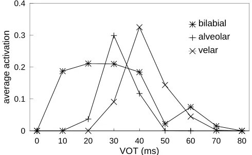
An important finding of Liberman et al. (1958) was that the voicing boundary depended systematically on place of ar-ticulation. In subsequent work, Lisker and Abramson (1970) found that as the place of articulation moves back in the vocal tract from bilabial (for a / ba–pa / VOT continuum) through alveolar (/da–ta /) to velar (/ga–ka /), so the bound-ary moves from about 25 ms VOT through about 35 ms to approximately 42 ms. Why this should happen is uncertain. For instance, Kuhl (1987 ) writes: “We simply do not know why the boundary “moves”.” (p. 365). One important impli-cation, however, is that CP is more than merely bisecting a continuum, otherwise the boundary would be at mid-range in all three cases.
At the time of the early Haskins work, and for some years thereafter, CP was thought to reflect a mode of perception special to speech (e.g., Liberman et al., 1957, 1967; Studdert-Kennedy, Liberman, Harris and Cooper, 1970) in which the listener somehow made reference to production. It was sup-posed that an early and irreversible conversion took place of the continuous sensory representation into a discrete, sym-bolic code subserving both perception and production (motor
theory). Thus, perception of consonants is supposedly more categorical than that of steady-state vowels because the
ar-ticulatory gestures that produce the former are more discrete than the relatively continuous gestures producing the latter.
Although there is little or no explicit mention of Weber’s law in early discussions of motor theory, its violation is one of the aspects in which CP was implicitly supposed to be spe-cial. Also, at that time, CP had not been observed for stimuli other than speech, a situation which was soon to change. Ac-cording to Macmillan, Braida and Goldberg (1987), however, “all . . . discrimination data require psychoacoustic explana-tion, whether they resemble Weber’s Law, display a peak, or are monotonic” (p. 32). In spite of attempts to modify it suit-ably (e.g., Liberman and Mattingly, 1985, 1989; Liberman, 1996), the hypothesis that CP is special to speech has been unable to bear the weight of accumulating contrary evidence. One strong line of contrary evidence comes from psy-choacoustic investigations, notably that of Kuhl and Miller (1978), using non-human animal listeners who “by def-inition, [have] no phonetic resources” (p. 906). These workers trained four chinchillas to respond differentially to the 0 ms and 80 ms endpoints of a synthetic VOT contin-uum as developed by Abramson and Lisker (1970). They then tested their animals on stimuli drawn from the full
3As pointed out to us by Michael Studdert-Kennedy (personal
Figure 1. Mean identification functions obtained for bilabial,
alve-olar and velar synthetic VOT series for human listeners and chin-chillas. Smooth curves have been fitted to the raw data points by probit analysis. Reprinted with permission from Kuhl and Miller, “Speech perception by the chinchilla: Identification functions for synthetic VOT stimuli”, Journal of the Acoustical Society of
Amer-ica, 63(3), March 1978, 905–917. Copyright 1978 Acoustical
Soci-ety of America.
0 to 80 ms range. Four human listeners also labeled the stimuli for comparison. Kuhl and Miller found “no signif-icant differences between species on the absolute values of the phonetic boundaries . . . obtained, but chinchillas pro-duced identification functions that were slightly, but sig-nificantly, less steep” (p. 905). Figure 1 shows the mean identification functions obtained for bilabial, alveolar and velar synthetic VOT series (Kuhl and Miller’s Figure 10). In this figure, smooth curves have been fitted to the raw data points (at 0, 10, 20, . . . 80 ms). Subsequently, working with macaques, Kuhl and Padden (1982, 1983) confirmed that these animals showed increased discriminability at the phoneme boundaries. Although animal experiments of this sort are methodologically challenging, and there have been difficulties in replication (e.g., Howell, Rosen, Laing and Sackin, 1992 working with chinchillas), the convergence of human and animal data in this study has generally been taken as support for the notion that general auditory processing and/or learning principles underlie this version of CP.
The emerging classical characterization of CP has been neatly summarized by Treisman, Faulkner, Naish and Ros-ner (1995) as encompassing four features: “a sharp cat-egory boundary, a corresponding discrimination peak, the predictability of discrimination function from identification, and resistance to contextual effects” (p. 335). These authors go on to critically assess this characterization, referring to “the unresolved difficulty that identification data usually pre-dict a lower level of discrimination than is actually found” (pp. 336–7) as, for example, in the work of Liberman et al. (1957), Studdert-Kennedy et al. (1970), Macmillan et al. (1977) and Pastore (1987a). They also remark on the
! "#$"%& '(
)*!+"%&
,.-/01$023 465
-78902:3
;
<>=
?
@BACDFEHGEI
JBKLMFNHONP
QSR!T$UVWSTR
XSY!Z$[\]SZY ^`_abcd
e$fhg
ikjml
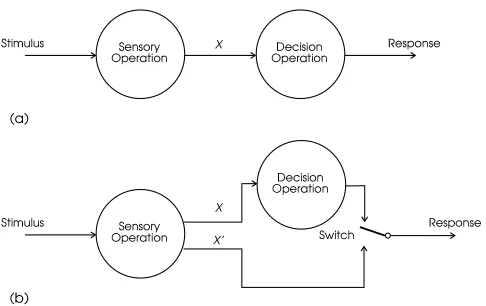
Figure 2. (a) The transformation of stimulus to response can be seen as a two-stage process of a sensory operation followed by a decision operation. This is consistent with signal detection theory’s separation of sensitivity and response bias measures. Redrawn from Massaro, 1987b. (b) In Fujisaki and Kawashima’s dual-process the-ory, there are two routes from sensory processing to decision: one continuous (X) and the other discrete (Xn).
cessity to qualify “Studdert-Kennedy et al.’s claim that con-text effects [and other sequential dependencies] are weak or absent in categorical perception” (see also Healy and Repp, 1982). We will take the classical characterization of CP to encompass only the first three aspects identified above, given the now rather extensive evidence for context effects and se-quential dependencies (e.g., Brady and Darwin, 1978; Diehl, Elman and McCusker, 1978; Rosen, 1979; Repp and Liber-man, 1987; Diehl and Kluender, 1987) which can shift the category boundary.4
Signal Detection and Criterion-Setting Theories
The pioneering Haskins work on phonetic categorization took place at a time when psychophysics was dominated by threshold models and before the influence of signal detection theory (Green and Swets, 1966; Macmillan and Creelman, 1991) was fully felt. Analyses based on signal detection the-ory (SDT) differ from classical views of CP in two respects. First, SDT clearly separates measures of sensitivity (d
o
) from measures of response bias (β). Second, the two views differ in details of how discrimination is predicted from identifica-tion, with labeling playing a central role in both aspects of performance in the classical view. We deal with the latter point in some detail below; brief remarks on the first point follow immediately.
Figure 2(a) (after Massaro, 1978b) shows the transfor-mation of stimulus to response in an identification or
dis-4However, the magnitude of context effects varies greatly with
crimination task as a two-stage process: sensory operation followed by decision operation. This is obviously consis-tent with SDT’s separation of sensitivity factors (having to do with sensory perception) and response bias (having to do with decision processes). The importance of this in the current context is that classical notions of CP are ambigu-ous about which of the representations are categorical: The information passed between sensory and decision processes (labeled X in the figure) could be categorical or continuous. In the latter case, this still allows the response to be categor-ical, but this is not CP in Massaro’s view because the cate-gorization does not occur at the sensory/perceptual stage: He prefers the term categorical partition. Emphasizing this dis-tinction, Massaro (1987a) writes, “I cannot understand why categorization behavior was (and continues to be) interpreted as evidence for categorical perception. It is only natural that continuous perception should lead to sharp category bound-aries along a stimulus continuum” (p. 115). (See also Hary and Massaro, 1982, and the reply of Pastore, Szczesiul, Wiel-gus, Nowikas and Logan, 1984).
According to SDT, X represents a continuous decision variate. In the simplest case, there are two kinds of presenta-tion (historically called signal and signal-plus-noise) and X is unidimensional. The two classes of presentation give rise to two normal distributions of equal variance, one with mean zero and the other with mean d
o
. Stimuli are then judged to be from one class or the other according to whether they give rise to an X value which is greater than or less than some internal criterion. However, as detailed by Macmil-lan et al. (1977) and reviewed below, the paradigms used in the study of CP have generally been more complex than this simple case.
Is the internal criterion fixed or can it shift as experi-ence changes? This question has been addressed in the recent work of Treisman et al. (1995) who apply the ear-lier criterion-setting theory (CST) of Treisman and Williams (1984) to CP. According to CST, a sensory system resets the response criterion between each trial according to “the latest information available to it, about its own sensory per-formance and the environment” (p. 337), leading to sequen-tial dependencies. The relevance to CP had been noted by Elman (1979) who suggested that consonant adaptation ef-fects might be due to such criterion shifts. When applied to ABX discrimination, CST “is shown to fit the data from the literature” (Treisman et al., 1995, p. 334), in that a peak occurs at the category boundary. This is essentially because CST shares the basic assumptions of the classical Haskins model (p. 345), which also predicts (from labeling) a peak as described below. Moreover, the absolute value of the ob-served discrimination performance is close to that predicted by CST. This is not the case with the Haskins model, which predicts a lower performance than is actually observed, as discussed immediately below. The better fit achieved by CST relative to the Haskins model is attributed to the former’s ad-ditional criterion-setting assumptions.
Prediction of Discrimination from Identification
In the classical Haskins view, discrimination in an ABX task (as traditionally used in CP studies) is based on covert labeling. First A is labeled covertly (in the sense that the sub-ject is not required to report this judgment to the investigator as in overt identification), then B, then X: If the A and B labels are different, the subject responds X is A or X is B according to X’s label, otherwise the subject guesses. On this basis, ABX discrimination is predictable from identifi-cation. Indeed, one of the criticisms of this paradigm (e.g., Pisoni and Lazarus, 1974; Massaro and Oden, 1980) is that it promotes identification/labeling behavior, so arguably pro-moting categorization behavior also. For judgements involv-ing just two categories, where the prior probability of each is equal, the proportion correct in discrimination is predicted as
P
p
Cqsr 0t5 u1v
p
pA
w
pBq
2xzy
(1)
where pA is the probability of identifying the A stimulus as one of the two categories, pB is the probability of identify-ing the B stimulus as that same category, and the guessidentify-ing probability is 0.5 (Liberman et al., 1957; Macmillan et al., 1977). It is well-known that this model predicts discrimi-nation which is almost invariably lower than that observed. CP theorists have usually played down this discrepancy by emphasizing the correlation between the predicted and ob-served curves—that is, their similar, non-monotonic shape and the fact that they peak at approximately the same (bound-ary) point.
Massaro (1987a) writes, “For some reason, the discrep-ancy has never been a deterrent for advocates of cate-gorical perception nor a central result for any alternative view” (p. 91). However, the dual-process model of Fujisaki and Kawashima (1969, 1970, 1971) does indeed effectively take this discrepancy as the basis of an alternative view, in which both a continuous (auditory) and a categorical
(pho-netic) mode of processing co-exist (Figure 2(b)). If the
sub-ject fails to label A and B differently via the categorical route then, instead of guessing, the continuous (but decay-ing) representations of A and B are consulted. According to Macmillan et al. (1977, p. 454), the extent to which Equa-tion 1 underestimates discriminaEqua-tion determines the weight to be given to each process so as to fit the data best. They crit-icize dual-process theory for “its embarrassing lack of parsi-mony” (p. 467), however, in that everything that can be done via the discrete route (and more) can also be achieved via the continuous route. The theory does, however, have other strengths. It can explain, for instance, the effect that memory requirements of the experimental procedure have on CP on the basis that the two processes have different memory-decay properties.
Macmillan et al. point out that the Haskins model is tac-itly based on low threshold assumptions5, arguing that mere
5In threshold theories (Luce, 1963; Macmillan and Creelman,
correlation between observed discrimination and that pre-dicted from identification is inadequate support for the no-tion of CP. By contrast, they characterize CP on the ba-sis of signal detection theory, in terms of the equivalence of discrimination and identification. The essential defining characteristic of CP is then considered to be the equivalence of identification d
o
, found using the approach proposed by Braida and Durlach (1972) for auditory intensity perception, and discrimination d
o
. The Braida and Durlach model as-sumes a distribution corresponding to each point on the con-tinuum, and then finds a d
o
for each adjacent pair of distri-butions. If we can find a d
o
corresponding to the same pair of distributions in ABX discrimination, then these two sen-sitivity measures should be equal if discrimination is indeed predictable from identification.
To avoid the low threshold assumptions of a discrete set of internal states, Macmillan et al. extended Green and Swets’ earlier (1966) derivation of d
o
from yes-no and two-interval forced choice (2IFC) psychophysical tasks to the somewhat more complicated ABX task. It was analyzed (pp. 458– 9) as a 2IFC subtask (to determine if the standards are in the order {AB| or {BA|
6), followed by a yes-no subtask.
This is described as “a continuous (SDT) model for cate-gorical perception” (p. 462). This view of the importance of continuous information to CP is gaining ground over the classical characterization of CP. For instance, Treisman et al. (1995) state that “CP resembles standard psychophysical judgements” (p. 334) while Takagi (1995) writes, “In fact, the signal detection model is compatible with both categor-ical and continuous patterns of identification/discrimination data” (p. 569).
Neural Models of CP: A Review
In this section, we present a historical review of neural models of CP.
The Brain-State-in-a-Box
Early neural models of categorical perception were es-sentially based on associative memory networks—one of the few kinds of net attracting any kind of interest in the “dark ages” (see Note 2) before the discovery of the error back-propagation algorithm (Rumelhart, Hinton and Williams, 1986). (See Kohonen, 1977, and Hinton and Anderson, 1981, for extensive contemporary reviews of parallel mod-els of associative memory and Anderson, 1995, for a more recent introductory treatment.) This is quite a natural model for CP in many ways. An associative net is addressed with some partial or noisy pattern and retrieves the corresponding noise-free canonical pattern, or prototype. This is akin to a pure or classical form of CP whereby a non-prototypical stimulus is replaced in memory by its prototype (from which it is consequently indistinguishable).
We will take Anderson et al.’s (1977) paper as the start-ing point for our review of neural models of CP. We note, however, that this selection may be contentious. Gross-berg, for example, also has a legitimate claim to be the
originator of this line of research with his very early pa-pers on neural models of psychological functions (Grossberg, 1968a, 1968b, 1969) although Anderson’s work on associa-tive memory dates back at least as far (viz., Anderson, 1968; see Grossberg, 1987, and Carpenter, Grossberg and Rosen, 1991a; 1991b, for more recent developments.) We prefer the Anderson et al. model because of its greater simplicity and perspicacity, and its more direct and obvious use in modeling human psychophysical data.
Anderson, Silverstein, Ritz and Jones (1977) consider net-works of neurons7 which “are simple analog integrators of
their inputs” (p. 416). They extend the earlier work men-tioned above (e.g., Anderson, 1968) in two main ways. It had previously been assumed (p. 413) that:
1. nervous system activity could be represented by the pat-tern of activation across a group of cells;
2. different memory traces make use of the same synapses;
3. synapses associate two patterns by incrementing synap-tic weights in proportion to the product of pre- and post-synaptic activities.
The form of learning implied in 3 is in effect correlational, and has been called Hebbian by many workers. As the neu-rons have linear activation functions, a form of linear correla-tion is computed, making the net amenable to analysis using linear systems theory as follows.
Suppose N-dimensional input pattern vectors fi are to be associated with M-dimensional output pattern vectors gi. A net is created with N input units and M output units. In accordance with point 2 above, f and g are to be represented by the patterns of activation across the input and output units respectively. Then, according to the learning scheme, the
(M } N) connection matrix A of synaptic weights between
the two sets of units is incremented by
Air g
ig
T i
y
(2)
where T denotes the vector transpose. In this way, the over-all connectivity matrix is determined as Ar ∑
iAi, summed over all I input patterns. If all inputs are mutually orthogonal, the output for any fkwill be
Afk r I
∑
i~ 1
Aifk
r Akfkv
∑
i~ k
Aifk
r gkf T
kfkv
∑
i~ k
gif T
ifk by Equation 2
∝ gky
the thresholds themselves set the limits to detection, and errors on
noise trials arise only from guessing. In low threshold theory, the
limit on performance is set by a factor other than the threshold, such as noise (Pastore, 1987b, p. 36).
6We use angled braces (
F) to denote an actual presentation dyad or triad (for which X cannot be ambiguous), in contrast to ABX which is the name of the paradigm.
since, by the definition of orthogonality:
fTifjr B fi
B
2 i
r j
0 otherwiset
Hence, the system operates as a perfect associator in this case: The direction of the output vector is identical to that of the associated input vector. (The length, however, is mod-ified by the length of the input vector and will also depend on the number of repetitions of that input in accordance with Equation 2.) When the inputs are not orthogonal, the net will produce noise as well as the correct output but it will still be “quite usable” (p. 417).
To convert this linear pattern-association net into a model of CP, Anderson et al. made two extensions. The first was to discard the M distinct output units and to introduce pos-itive feedback from the set of N input neurons onto itself. The (N} N) matrix bf A (which they now call the “feedback matrix”) is made symmetric in this case, so that the synaptic weight between units i and j is equal to that between units j and i: aij= aji. For the case of arbitrary (non-orthogonal) in-puts, it is shown (p. 424) that (provided their average is zero) the inputs are a linear combination of the eigenvectors of the feedback matrix A, and all eigenvalues are positive.
The introduction of positive feedback makes the system potentially unbounded in that activations can now grow with-out limit. The second extension overcomes this problem by allowing the individual neurons to saturate at an activation
of C. That is, the activation function of each neuron is
linear-with-saturation. Thus, in use, all units are eventually driven into saturation (either positive or negative in sense) and the net has stable states corresponding to some (possibly all) of the corners of a hypercube (box) in its N-dimensional state space. (Of course, not all corners are necessarily sta-ble.) For this reason, the model was called
brain-state-in-a-box (BSB). Considered as vectors in the state space, these
corners are the eigenvectors of A and can be identified, in psychological terms, with the distinctive features of the sys-tem (p. 425). For each such stable state, there is a region of attraction in state space such that if an input initially pro-duces an output in this region, that output will evolve over time to reach that stable state, where it will remain.
Used as a model of CP, the inputs (i.e., the fi) are asso-ciated with themselves during training, that is, during com-putation of the (N} N) matrix A@. This is an essentially unsupervised operation. However, if the training patterns are labeled with their pattern class, the corners of the box can be similarly labeled according to the input patterns that they attract. (There is, of course, no guarantee that all corners will be so labeled. Corners which remain unla-beled correspond to rubbish states in the jargon of associa-tive networks.) Thereafter, an initial noisy input (consist-ing of a linear sum of eigenvectors) within the region of attraction of a labeled corner will evoke an output which is a canonical or prototypical form corresponding to the eigenvector of the input with the largest eigenvalue. An-derson et al. (pp. 430–433) present a simulation of CP in which their neural model performed two-class identification
zz
B
$$$$$$`$B$`$B$ $$$``$$$$`$`
(a)
0 0.2 0.4 0.6 0.8 1
vector number
proportion labeled `0'
0 1 2 3 4 5 6 7 8 9 10 11 12 13 14 15
SD = 0.0 SD = 0.4 SD = 0.7
(b)
Figure 3. (a) eight-dimensional system with two orthogonal length-two eigenvectors used in the simulation of CP based on the brain-state-in-a-box neural model. Inputs consisted of 16 equally spaced length-one vectors as shown, with added noise. Redrawn from Anderson et al. (1977). (b) Response of model for the simu-lated identification task with 1,000 presentations at each noise con-dition: standard deviation 0.0, 0.4 or 0.7.
and ABX discrimination tasks. The two prototypes (eigen-vectors) were the eight-dimensional orthogonal vectors of length-two in the directions
p
1y 1y
1y 1y
w
1y
w
1y
w
1y
w
1q and
p
1y 1y
w 1
y
w 1
y
1y 1y
w 1
y
w 1
q respectively (Figure 3(a)). These were used to set the weights as detailed above. Inputs to the model then consisted of 100 repetitions of 16 length-one vectors equally spaced between the prototype eigenvectors, with added zero-mean Gaussian noise according to one of four conditions: The standard deviation (SD) of the noise was either 0.0, 0.1, 0.2 or 0.4.
acti
p
tqsr α
p
extinputiqv β
p
intinputiq
y
(3)
where extinputiand intinputiare, as their names clearly sug-gest, the external input to unit i and the internal (feedback) input to the same unit. A decay term,
∆actir α
p
extinputiqv β
p
intinputiq
w
p
decayqacti
y
can be incorporated into the model, which tends to restore activation to a resting level of zero. Throughout this work,
decay was set to 1 so that the activation is given simply by
Equation 3.
For the replication of Anderson et al.’s simulation, the ex-ternal scale factor α and internal scale factor β were both set at 0.1. The saturation limit for the neurons was set at
C = 1. Self connections between neurons were allowed. We also found it necessary to use rather more noise power than Anderson et al. did. We believe this is because our use of 1,000 test patterns (in place of Anderson et al.’s 100) makes our results less affected by small-sample effects. Thus, our noise conditions were SD = 0.0, 0.4 and 0.7.
In all noise-free cases, the system converged to one of its two stable, saturating states for all 1,000 inputs. For the added noise conditions, there was only a very small likelihood of convergence to an unlabeled corner (rubbish state). This occurred for approximately 1% of the inputs when SD = 0.4 and for about 6% when SD = 0.7. Figure 3(b) shows the identification results obtained by noting the pro-portion of inputs which converge to the saturating state cor-responding to endpoint 0. For the no-noise condition, cate-gorization is perfect with the class boundary at the midpoint between the prototypes. For the noise conditions, SD = 0.4 and SD = 0.7, the labeling curves are very reasonable approx-imations to those seen in the classical CP literature. Overall, this replicates the essential findings of Anderson et al.
Consider next the ABX discrimination task. Anderson et al. considered two inputs to the net to be discriminable if they converged to different stable states. (Note that as Anderson et al. are considering a simple two-class problem with con-vergence to one or other of the two labeled states, and no rubbish states, they are never in the situation of having A, B and X all covertly labeled differently, as can conceivably happen in reality.) If they converged to the same stable state, a guess was made with probability 0.5, in accordance with Equation 1. This means that discrimination by the net is ef-fectively a direct implementation of the Haskins model. In-deed, Anderson et al. observed a distinct peak at midrange for their intermediate-noise condition, just as in classical CP. Finally, they obtained simulated reaction times by noting the number of iterations required to converge to a stable, saturat-ing state. As in classical CP (e.g., Pisoni and Tash, 1974), there was an increase in reaction time for inputs close to the category boundary for the intermediate noise condition, rel-ative to inputs more distant from the boundary. Again, we have replicated these findings (results not shown).
In support of the assertion that the model is “quite us-able” when the inputs are not orthogonal, Anderson (1977, pp. 78–83) presents an example in which the BSB model is
used to categorize vowel data (see also Anderson, Silver-stein and Ritz, 1977). 12 Dutch vowels were represented by eight-dimensional vectors, each element measuring the en-ergy within a certain frequency band of an average, steady-state vowel. It is highly unlikely that these inputs are mutu-ally orthogonal, yet “when learning ceased, each vowel was assigned to a different corner” (p. 81). Indeed, as mentioned earlier, non-orthogonality can act as noise, thus preventing (unrealistic) perfect categorization.
Anderson et al. (1977) conjecture that positive feedback, saturation and synaptic learning are “responsible for the in-teresting [categorization] effects in our simulations” (p. 433). With the benefit of hindsight, however, we now know (based on the extensive review material and new results below) that synthetic categorization can be obtained in a variety of neural models, even those lacking positive feedback and saturation. In this regard, the comments of Grossberg (1986) concern-ing saturation in the BSB model are apposite. He charged Anderson et al. with introducing a homunculus as a result of their “desire to preserve the framework of linear systems theory”. He continues: “No physical process is defined to justify the discontinuous change in the slope of each variable when it reaches an extreme of activity . . . The model thus invokes a homunculus to explain . . . categorical perception” (pp. 192–194).
In our view, however, a homunculus is an unjustified, im-plicit mechanism which is, in the worst case, comparable in sophistication and complexity to the phenomenon to be ex-plained. By contrast, Anderson et al. postulate an explicit mechanism (firing-rate saturation) which is both simple and plausible in that something like it is a ubiquitous feature of neural systems. In the words of Lloyd (1989), “Homunculi are tolerable provided they can ultimately be discharged by analysis into progressively simpler subunculi, until finally each micrunculus is so stupid that we can readily see how a mere bit of biological mechanism could take over its du-ties” (p. 205). Anderson et al. go so far as to tell us what this “mere bit of biological mechanism” is—namely, rate saturation in neurons. (See Grossberg, 1978, and the reply thereto of Anderson and Silverstein, 1978, for additional dis-cussion of the status of the non-linearity in the Anderson et al. BSB model: see also B´egin and Proulx, 1996, for more re-cent commentary.) To be sure, the discontinuity of the linear-with-saturation activation function is biologically and math-ematically unsatisfactory, but essentially similar behavior is observed in neural models with activation functions having a more gradual transition into saturation (as detailed below).
The T
RACEModel
con-sistent with a given interpretation of the input have excita-tory connections, while those within a level that are contra-dictory have inhibitory connections—that is, processing is
competitive.
Strictly speaking, TRACEis as much a model of lexical ac-cessing as of speech perception per se, as the existence of the word units makes plain. McClelland and Elman assumed an input in terms of something like ‘distinctive features’, which sidesteps important perceptual questions about how the dis-tinctive features are derived from the speech signal and, in-deed, about whether this an appropriate representation or not. In their 1986 Cognitive Psychology paper, McClelland and Elman describe TRACE II which, they say, is “designed to account primarily for lexical influences in phoneme percep-tion” using “mock speech” as input (p. 13). However, they also refer to TRACE I which is “designed to address some of the challenges posed by the task of recognizing phonemes in real speech” and cite Elman and McClelland (1986) for further details. Unfortunately, TRACEI does not feature real speech input either.
Top-down effects are manifest through the lexical status (or otherwise) of words affecting (synthetic) phoneme per-ception and thereby (synthetic) feature perper-ception also. Al-though TRACE has been used to simulate a variety of ef-fects in speech perception, we concentrate here on its use to model CP.
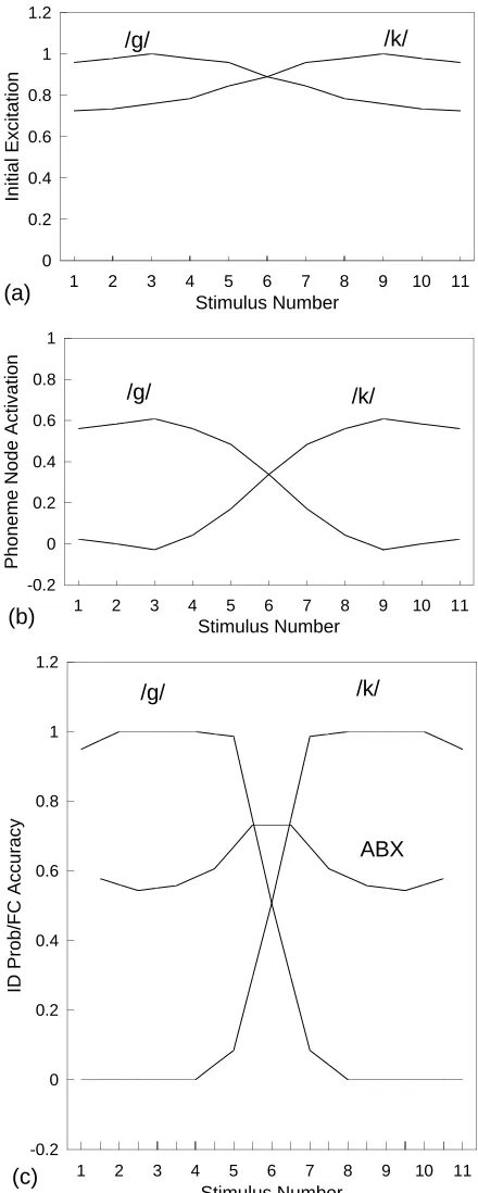
An 11-step /g /–/ k / continuum was formed by interpolat-ing the feature values: namely, voice onset time (VOT) and the onset frequency of the first formant, F1. The endpoints of the continuum (stimuli 1 and 11) were more extreme than prototypical /g / and / k /, which occurred at points 3 and 9, respectively. The word units were removed, thus excluding any top-down lexical influence, and all phoneme units other than /g / and / k / were also removed. Figure 4(a) shows the initial activations (at time step t = 1) at these two units as a function of stimulus number. As can be seen, there is a clear trend for the excitation (which is initially entirely bottom-up) to favor /g / at low stimulus number but / k / at high stimulus number. The two curves cross at stimulus number 6, indicat-ing that this condition is maximally ambiguous (i.e., this is the phoneme boundary). However, the variation is essentially continuous rather than categorical, as shown by the relative shallowness of the curves. By contrast, after 60 time steps, the two representations are as shown in Figure 4(b). As a re-sult of mutual inhibition between the /g / and / k / units, and possibly of top-down influence of phoneme units on featu-ral units also, a much steeper (more categorical) response is seen.
This appears to be a natural consequence of the compe-tition between excitatory and inhibitory processing. Many researchers have commented on this ubiquitous finding. For instance, Grossberg (1986) states, “Categorical perception can . . . be anticipated whenever adaptive filtering interacts with sharply competitive tuning, not just in speech recogni-tion experiments” (p. 239).
McClelland and Elman go on to model overt labeling of the phonemes, basing identification on a variant of Luce’s (1959) choice rule. The result is shown in Figure 4(c), which
/g/
0 0.2 0.4 0.6 0.8 1 1.2
Stimulus Number
Initial Excitation
1 2 3 4 5 6 7 8 9 10 11
/g/ /k/
(a)
-0.2 0 0.2 0.4 0.6 0.8 1
Stimulus Number
Phoneme Node Activation
1 2 3 4 5 6 7 8 9 10 11
/k/ /g/
(b)
/g/
-0.2 0 0.2 0.4 0.6 0.8 1 1.2
Stimulus Number
ID Prob/FC Accuracy
1 2 3 4 5 6 7 8 9 10 11
/k/ /g/
ABX
(c)
Figure 4. Categorical perception in the TRACEmodel: (a) Initial activation of the /g / and / k / units arising from bottom-up influence of the feature units, at time step t = 1. (b) Activations at time step
t = 60. (c) Labeling functions after post-processing using Luce’s
also depicts the ABX discrimination function. The choice rule involves setting a constant k (actually equal to 5) which acts as a free parameter in a curve-fitting sense. Quinlan (1991) accordingly makes the following criticism of TRACE: “Indeed, k determined the shape of the identification func-tions . . . A rather uncharitable conclusion . . . is that the model has been fixed up to demonstrate categorical percep-tion . . . Categorical perceppercep-tion does not follow from any of the a priori functional characteristics of the net” (p. 151). It is also apparent that the obtained ABX discrimination curve is not very convincing, having a rather low peak relative to those found in psychophysical experiments.
We consider finally the relation between discrimination and identification in TRACE. McClelland and Elman point out that discrimination in real CP is better than predicted from identification and that TRACEalso “produces this kind of approximate categorical perception” (p. 47). The mech-anism by which this happens is by an interaction of the bottom-up activations produced by the speech input with the top-down activations. According to the authors, the former decay with time, but not entirely to zero, whereas the latter produce a more canonical representation with time but do not completely overwrite the input with its prototype (and the time course of these interactions gives a way of predicting the increase in reaction time for stimuli close to the category boundary.) The authors remark on the practical difficulty of distinguishing between this feedback explanation and a dual-process explanation.
Back-propagation
As is well known, the field of neural computing received a major boost with the discovery of the error back-propagation algorithm (Rumelhart, Hinton and Williams, 1986) for train-ing feedforward nets with hidden units, so-called multilayer perceptrons (MLPs). It is therefore somewhat surprising that back-propagation learning has not figured more widely in studies of synthetic CP. We have used this algorithm as the basis for modeling the categorical perception of both speech (dealt with in the next section) and artificial stimuli (dealt with here).
Many workers (Bourlard and Kamp, 1988; Elman and Zipser, 1988; Baldi and Hornik, 1989; Hanson and Burr, 1990) have observed that feedforward auto-associative nets8
with hidden units effectively perform a principal compo-nent analysis of their inputs. Harnad, Hanson and Lu-bin (1991) exploited auto-association training to produce a
precategorization discrimination function. This was then
re-examined after categorization training to see if it had warped. That is, a CP effect was defined as a decrease in within-category inter-stimulus distances and/or an increase in between-category inter-stimulus distances relative to the baseline of auto-association alone. The stimuli studied were artificial—namely, different representations of the length of (virtual) lines—and the net’s task was to categorize these as
short or long.
A back-propagation net with eight input units, a single hidden layer of 2 to 12 units and 8 or 9 output units was
used. The 8 different input lines were represented in 6 different ways, to study the effect of the iconicity of the input coding (i.e., how analog, non-arbitrary, or structure-preserving it was in relation to what it represented)9.
Af-ter auto-association training (using eight output units), the trained weights between hidden layer and output layer were reloaded, the input to hidden layer weights were set to small random values, and training recommenced. The net was given a double task: auto-association (again) and catego-rization. For the latter, the net had to label lines 1 to 4 (for instance) as short and 5 to 8 as long. This required an addi-tional output, making nine in this case.
Strong CP effects (with warping of similarity space in the form of increased separation across the category bound-ary and compression within a category) were observed for all input representations: The strongest effect was obtained with the least iconic, most arbitrary (place) code. The categorization task was very difficult to learn with only two hidden units, h = 2. With more hidden units, how-ever, the pattern of behavior did not change with increas-ing h (3 to 12). This is taken to indicate that CP is not merely a byproduct of information compression by the hid-den layer. Nor was CP a result of overlearning to extreme values, because the effect was present (albeit smaller) for larger values of the epsilon (ε) error criterion in the back-propagation algorithm. A test was also made to determine if CP was an artifact of re-using the weights for the pre-categorization discrimination (association) for the auto-association-plus-categorization. Performance was averaged over several precategorization nets, and compared to perfor-mance averaged over several different auto-association-plus-categorization nets. Again, although weaker and not always present, there was still evidence of synthetic CP.
A final test concerned iconicity and interpolation: Was the CP restricted to trained stimuli, or would it generalize to untrained ones? Nets were trained on auto-association the usual way, and then, during categorization training, some of the lines were left untrained (say, line 3 and line 6) to see whether they would nevertheless warp in the ‘right’ direc-tion. Interpolation of the CP effects to untrained lines was found, but only for the coarse-coded representations.
A “provisional conclusion” of Harnad et al. (1991) was that “whatever was responsible for it, CP had to be something very basic to how these nets learned”. In this and subsequent work (Harnad, Hanson and Lubin, 1995), the time-course of the training was examined and three important factors in
gen-8Here, the term auto-associative refers to multilayer
feedfor-ward nets with hidden units trained to reproduce their inputs as outputs. This is distinct from auto-associative feedback nets like the BSB model in which there are no hidden units and the input and
output units are physically identical.
9The reader might object that lines of differing length are not
erating synthetic CP were identified:
1. maximal interstimulus separation induced during auto-association learning with the hidden-unit representations of each (initially random) stimulus moving as far apart from one another as possible;
2. stimulus movement to achieve linear separability dur-ing categorization learndur-ing, which undoes some of the sepa-ration achieved in 1 above, in a way which promotes within-category compression and between-within-category separation;
3. inverse-distance “repulsive force” at the category boundary, pushing the hidden-unit representation away from the boundary and resulting from the form of the (inverse ex-ponential) error metric which is minimized during learning.
One further factor—the iconicity of the input codings— was also found to modulate CP. The general rule is that the further the initial representation is from satisfying the parti-tion implied in 1 to 3 above (i.e., the less iconic it is), the stronger is the CP effect. Subsequently, Tijsseling and Har-nad (1997) carried out a more detailed analysis focusing par-ticularly on the iconicity. Contrary to the report of Harnad et al. (1995), they found no overshoot as in 2 above. They con-clude: “CP effects usually occur with similarity-based cate-gorization, but their magnitude and direction vary with the set of stimuli used, how [these are] carved up into categories, and the distance between those categories”.
This work indicates that a feedforward net trained on back-propagation is able (despite obvious dissimilarities) to replicate the essential features of classical CP much the way the BSB model of Anderson et al. (1977) does. There are, however, noteworthy differences. The most important is that Harnad et al.’s back-propagation nets are trained on interme-diate (rather than solely on endpoint) stimuli. Thus, gener-alization testing is a more restricted form of interpolation. Also (because the feedforward net has no dynamic behavior resulting from feedback), reaction times cannot be quite so easily predicted as Anderson et al. do (but see below.)
Competitive Learning and Category Detecting
Neurons
Goldstone, Steyvers and Larimer (1996) report on a labo-ratory experiment with human subjects in which stimuli from a novel dimension were categorically perceived. The stimuli were created by interpolating (morphing) seven curves be-tween two randomly selected bezier endpoint curves. The dimension is novel in that subjects are highly unlikely ever to have seen precisely those morphed shapes before. The major interest in the context of this paper is that Goldstone et al. also present a neural model (a form of radial-basis function net) which qualitatively replicates the behavioral results.
The model has a layer of hidden neurons which become specialized for particular stimulus regions, thereby acting as “category detecting neurons” in the sense of Amari and Takeuchi (1978) or “feature detecting neurons” in the sense of Schyns (1991). This is done by adjusting the input-to-hidden (or position) weights. Simultaneously, associations between hidden/detector neurons and output (category) units are learned by gradient descent. As well as the feedforward
connections from input-to-hidden and from hidden-to-output units, there is feedback from the category units, which causes the detector units to concentrate near the category boundary. This works by increasing the position-weight learning rate for detectors that are neighbors of a detector that produces an improper categorization. Note that the whole activity pattern of the hidden detectors determines the activity of the cate-gory nodes. This in turn determines the error and, thus, the learning rate: No single detector can determine the learning rate (Mark Steyvers, personal communication, July 9, 1997). Goldstone et al. mention the similarity of the classification part of their model to ALCOVE(Kruschke, 1992). Like AL -COVE, the hidden nodes are radial-basis function units “acti-vated according to the psychological similarity of the stimu-lus to the exemplar at the position of the hidden node” (p. 23). The essential difference is that Goldstone et al.’s exemplar nodes are topologically arranged, and can move their posi-tion in input space through competitive learning of their po-sition weights.
Simulations were performed with input patterns drawn from 28 points on the morphed continuum. (Two-dimensional gray-scale drawings of the curves were con-verted to Gabor filter representations describing the inputs in terms of spatially organized line segments.) There were 14 hidden exemplar/detector neurons and 2 output/category neurons. Like the experiments with the human subjects, the simulations involved learning two different classifications according to different cut-offs along the novel dimension. In one condition (left split), the cut-off (boundary) was placed between stimuli 10 and 11; in the other condition (right split), it was placed between stimuli 18 and 19. In both cases, clas-sical CP was observed. Although Luce’s choice rule is ap-parently used in the Goldstone et al. model, it seems that the
k parameter which was treated by McClelland and Elman as
free in the TRACE model and adjusted to give CP, is here treated as fixed (at unity). The labeling probability showed a characteristic warping, with its 50% point at the relevant boundary. Discrimination between two stimuli was assessed by taking the Euclidean distance between their hidden-node activation patterns. This revealed a peak in sensitivity at or near the relevant category boundary.
Unfortunately, Goldstone et al. did not (and cannot) make a strict comparison of their human and simulation data, be-cause of the different numbers of curves in the two con-tinua studied. Recall that seven morphed curves constituted the continuum for the experiments with human participants, whereas a morphing sequence of 28 curves was used in the simulations. Such a comparison could have been very re-vealing for understanding synthetic CP. Nonetheless, there is sufficient coincidence of the form of their results in the two cases to show that neural nets can indeed make credible models of learned categorization.
The authors contrast their work with that of Anderson et al. (1977) and Harnad et al. (1995). In these other ap-proaches, they say, “each category has its own attractor”10so
10We prefer to reserve the term attractor to describe a stable state
that CP “occurs because inputs that are very close but fall into different categories will be driven to highly separated attrac-tors” (p. 248). In their net, however, detectors congregate at the category boundary, and thus “small differences . . . will be reflected by [largely] different patterns of activity”. These as-pects of their work are presented as potentially advantageous. However, they seem to run counter to the prevailing view in speech CP research according to which the paradigm “has overemphasized the importance of the phonetic boundary be-tween categories” (Repp, 1984, p. 320) at the expense of ex-ploring the internal structure of the categories in terms of an-chors and/or prototypes (e.g., Macmillan, 1987; Kuhl, 1991; Volaitis and Miller, 1992; Miller, 1994; Iverson and Kuhl, 1995; Guenter and Gjaja, 1996—but see Lotto et al., 1998).
Categorization of Stop
Consonants by Neural Networks
From the foregoing review, it is apparent that (given the right encoding schema for the inputs) neural models of CP have no real problem replicating the classical observations of a sharp labeling function and a peaked discrimination func-tion, at least for learned categorization. While there may sometimes be contrary suspicions (as when Luce’s choice rule is used in the TRACEmodel, or nets are trained to place the category boundary at a particular point on the input con-tinuum), the effects are sufficiently robust across a variety of different architectures and approaches to support the claim that they reflect the emergent behavior of any reasonably powerful learning system (see below). With the exception of the vowel categorization work using the BSB model (An-derson, 1977; Anderson et al., 1977), however, the neural models of synthetic CP reviewed thus far have all taken their inputs from artificial or novel dimensions, whereas the vast majority of real CP studies have used speech stimuli—most often stop consonants (or, more correctly, simplified analogs of such sounds). Our goal in this section is accordingly to consider the categorization of stop consonants by a variety of neural models. As mentioned earlier, an important aspect of the categorization of stop consonants is the shift of the category boundary with place of articulation. Thus, it is of considerable interest to ascertain if neural models of CP re-produce this effect as emergent behavior.
Stimuli and Pre-Processing
The stimuli used in this section were synthesized consonant-vowel syllables supplied by Haskins Laborato-ries, and nominally identical to those used by Kuhl and Miller (1978) which were developed earlier by Abramson and Lisker (1970). Stimuli very much like these, if not iden-tical, have been used extensively in studies of speech CP: they have become a gold standard for this kind of work. They consist of three series, digitally sampled at 10 kHz, in which VOT varies in 10 ms steps from 0 to 80 ms, simulating a series of English, prestressed, bilabial (/ ba–pa /), alveolar (/ da–ta /) and velar (/ ga–ka /) syllables. Each stimulus began with a release burst, and the two acoustic variables of aspi-ration duaspi-ration and F1 onset frequency were then varied
si-multaneously in order to simulate the acoustic consequences of variation in VOT. Strictly then, the VOT continuum is not unidimensional. However, as mentioned in Footnote 3, these two variables have often been thought to be perfectly correlated.
The stimuli were pre-processed for presentation to the var-ious nets using a computational model of the peripheral au-ditory system (Pont and Damper, 1991). The use of such sophisticated pre-processing obviously requires some justifi-cation. We know from above that the iconicity of the input representation to the network is important: the closer the rep-resentation to that ‘seen’ by the real observer the better. Also, there has long been a view in the speech research literature that CP reflects some kind of “restructuring of information” (Kuhl and Miller, 1978, p. 906) by the auditory system in the form of processing non-linearities. We wished accord-ingly to find correlates of CP in the neural activity of the auditory system, following Sinex and McDonald (1988) who write: “It is of interest to know how the tokens from a VOT continuum are represented in the peripheral auditory system, and whether [they] tend to be grouped in a way which pre-dicts the psychophysical results” (p. 1817). Also, as a step towards understanding the acoustic-auditory restructuring of information, we wished to discover the important acoustic features which distinguish initial stops. In the words of Nos-sair and Zahorian (1991), who used automatic speech recog-nition techniques for this purpose: “Such features might be more readily identifiable if the front-end spectral processing more closely approximated that performed by the human au-ditory system” (p. 2990). Full details of the pre-processing are described elsewhere (Damper, Pont and Elenius, 1990): Only a brief and somewhat simplified description follows.
The output of the auditory model is a neurogram (or
neu-ral spectrogram) depicting the time of firing of a set of
128 simulated auditory nerve fibers in response to each stim-ulus applied at time t = 0 at a simulated sound pressure level of 65 dB. Spacing of the filters in the frequency dimension is according to the Greenwood (1961) equation, corresponding to equal increments of distance along the basilar membrane. Because of the tonotopic (frequency-place) organization of auditory nerve fibers, and the systematic spacing of the filters across the 0 to 5 kHz frequency range, the neural spectro-gram is a very effective time-frequency representation. The high data rate associated with the full representation is dra-matically reduced by summing nerve firings (spikes) within time-frequency cells to produce a two-dimensional matrix. Some such data reduction is necessary in order to estimate reliably the parameters of the network model from sparse training data. Spikes are counted in a
p
12} 16q-bin region stretching from
w
25 ms to 95 ms in 10 ms steps in the time dimension and from 1 to 128 in steps of 8 in the frequency (fiber CF index) dimension. Thus, the nets have a maximum of 192 inputs. These time limits were chosen to exclude most (but not all) of the prestimulus spontaneous activity and the region where responses were expected to be entirely
acteristic of the vowel. The impact on synthetic CP of the number and placement of these time-frequency cells has not yet been investigated systematically, just because the initial scheme that we tried worked so well. Some prior thought was given to the resolutions chosen. The 10 ms width of the time bin corresponds approximately to one pitch period. The grouping into eight contiguous filters, in conjunction with equi-spacing according to the Greenwood equation, corre-sponds to a cell width which is an approximately constant fraction (about 0.7) of the critical bandwidth.
Since the auditory pre-processor is stochastic in nature (because of its simulation of mechanical-to-neural transduc-tion in the hair cells of the cochlea), repetitransduc-tions of the same input stimulus produce statistically different outputs. This fact is very convenient: It means that a sufficiently large data set for training the neural models can be generated simply by running the pre-processor repeatedly with the same input. In this work, 50 repetitions were used for each of the three (bi-labial, velar, alveolar) series to produce neural spectrograms for training and testing the nets.
Brain-State-in-a-Box Model
There was a distinct net for each of the (bilabial, alveolar, velar) stimulus series. The input data were first reduced to (approximately) zero-mean bipolar patterns by subtracting 5 from each value. This was sufficient to ensure that negative saturating states were appropriately used in forming attrac-tors, in addition to positive saturating states. Initially, simula-tions used all 192 inputs. A possible problem was anticipated as follows. The number of potential attractor states (corners of the box) in the BSB model grows exponentially with the number of inputs: In this case, we have 2192potential attrac-tors. Clearly, with such a large number, the vast majority of states must remain unlabeled. This will only be a problem, however, if a test input is actually in the region of attraction of such an unlabeled (rubbish) state. In the event, this did not happen. However, training was still unsuccessful in that the different endpoint stimuli (canonical voiced or 0 ms VOT, and canonical unvoiced or 80 ms VOT) were attracted to the same stable states: There was no differentiation between the different endpoints. This was taken as an indication that the full 192-value patterns were more similar to one another than they were different.
In view of this, the most important time-frequency cells were identified by averaging the endpoint responses and tak-ing their difference. The N cells with the largest associated absolute values were then chosen to form the inputs to an
N-input, N-unit BSB net. This is a form of
orthogonaliza-tion. Ideally, this kind of pre-analysis is best avoided: The neural model ought to be powerful enough in its own right to discover the important inputs. Preliminary testing indi-cated that results were not especially sensitive to the pre-cise value of N provided it was in the range somewhere be-tween about 10 and 40. A value of 20 was therefore cho-sen. These 20 most important time-frequency cells are lo-cated around the low-frequency region (corresponding to 200 to 900 Hz) just after acoustic stimulus onset where
voic-ing activity varies maximally as VOT varies. The precise time location of this region shifts in the three nets (bilabial, alveolar, velar) in the same way as does the boundary point. The nets were then trained on the 0 ms and 80 ms endpoints and generalization was tested on the full range of stimuli in-cluding the (unseen) intermediate (10 to 70 ms) stimuli.
Because of the relatively large number (100) of training patterns contributing to the feedback matrix (Equation 2) and hence to the weights, it was necessary to increase the neuron saturation limit markedly (to C = 20,000). The external scale factor was set at αr 0t1, and the internal scale fac-tor at βr 0t05. These values were arrived at by trial and error; network behavior was not especially sensitive to the precise settings. Again, self connections between neurons were allowed. It was found that the 0 ms (voiced) train-ing patterns were always assigned different corners from the 80 ms (unvoiced) patterns. During generalization testing, no rubbish states were encountered: Convergence was always to a labeled attractor. Moreover, the activation vector (after convergence) for the 0 ms stimuli was found to be the same after training for all three series (i.e., the voiced stimuli all shared the same attractors, irrespective of place of articula-tion). The same was true of the 80 ms (unvoiced) endpoint stimuli. (This would, of course, be a problem if the task of the net were to identify the place of articulation rather than the presence/absence of voicing.)
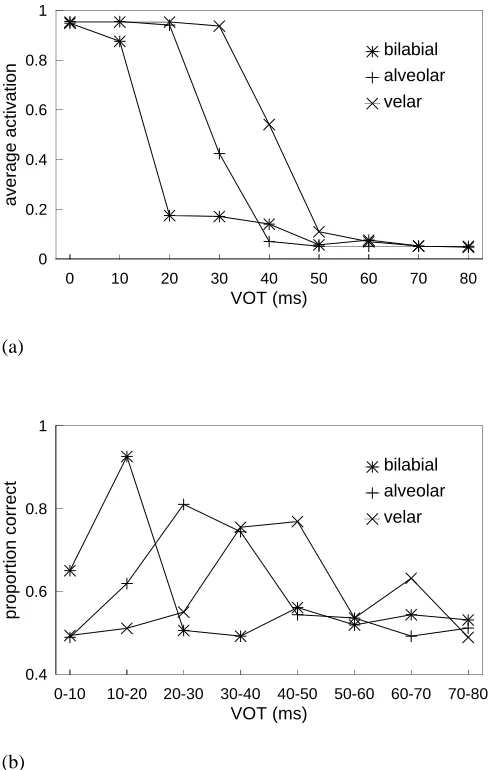
Figure 5(a) shows the identification function obtained by plotting the proportion of the 50 presentations which con-verged to a state labeled voiced for each of the three series; Figure 5(b) shows the one-step discrimination function (aver-aged over 1,000 presentations) obtained using the procedure of Anderson et al. (1977) as described in the Brain-State-in-a-Box subsection above. The results are clear and unequiv-ocal: Classical categorization is observed with a steep label-ing curve and an ABX discrimination peak at the category boundary. Although the labeling curve is rather too steep and the actual boundary values obtained are slightly low (by about 5 or 10 ms), the shift with place of articulation is qual-itatively correct. The finding of correct order of boundary placement was very consistent across replications with dif-ferent scale factors: We take this to be an indication of its significance. With these more realistic input patterns, there is no need to add noise as there was in the case of the artificial (vectors) input.
0 0.2 0.4 0.6 0.8 1
VOT (ms)
proportion labeled voiced
0 10 20 30 40 50 60 70 80
bilabial alveolar velar
(a)
0.4 0.6 0.8 1
VOT (ms)
proportion correct
0-10 10-20 20-30 30-40 40-50 50-60 60-70 70-80
bilabial alveolar velar
(b)
Figure 5. Categorical perception of voice-onset time in the brain-state-in-a-box model: (a) Labeling functions for bilabial, alveolar and velar series. Each point is an average of 50 presentations. (b) One-step ABX discrimination functions. Each point is an average of 1,000 presentations.
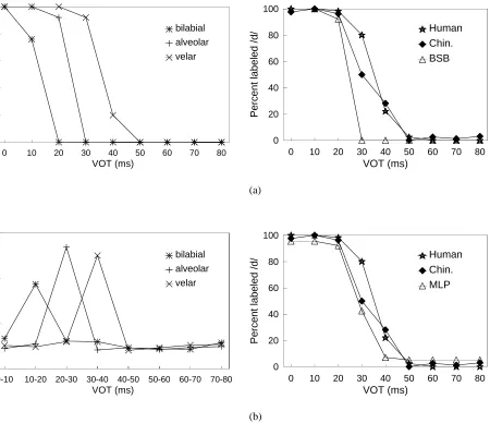
Miller’s animal and human alveolar labeling data was 10.5 percentage points.) Findings were similar in the case of the bilabial and velar stimuli.
Figure 7 shows the obtained one-step discrimination func-tion for the alveolar series, and that predicted on the basis of Equation 1. They are essentially identical, differing only in that the obtained function is contaminated by the sampling statistics of the guessing process.
Back-propagation Network
In light of the foregoing review, there are (at least) two ways that a model of synthetic CP based on back-propagation training of a feedforward net can be produced:
1. As with the BSB model (and paralleling the animal ex-periments of Kuhl and Miller, 1978), the net is trained on the
0 20 40 60 80 100
VOT (ms)
Percent labeled /d/
0 10 20 30 40 50 60 70 80
Human Chin. BSB
(a)
0 20 40 60 80 100
VOT (ms)
Percent labeled /d/
0 10 20 30 40 50 60 70 80
Human Chin. MLP
(b)
Figure 6. Composite labeling functions for the alveolar series for humans, chinchillas and neural networks. The human and animal data are taken from Kuhl and Miller (1978, their Figure 3) . (a) Brain-state-in-a-box neural model. (b) Multi-layer perceptron.
0 ms and 80 ms endpoints and generalization is then tested using the full range of VOT stimuli.
2. Using the auto-association paradigm of Harnad et al. (1991, 1995), hidden-unit representations resulting from pre-and post-categorization training are compared.
In this work, we have adopted approach 1, mostly because we have both psychophysical and synthetic (BSB model) data against which to assess our simulation. This was not the case for Harnad et al.’s artificial data, which accordingly required some other reference for comparison.