Gupta, Pankaj (2019): Neural information extraction from natural language text. Dissertation, LMU München: Fakultät für Mathematik, Informatik und Statistik

(1)

from Natural Language Text

Dissertation

an der Fakult¨at f¨ur Mathematik, Informatik und Statistik

der Ludwig–Maximilians–Universit¨at

M¨unchen

Pankaj Gupta

(2)

(3)

Zweitgutachter: Associate Prof. Dr. Ivan Titov, PhD

Drittgutachter: Assistant Prof. Dr. William Wang, PhD

Tag der Einreichung: 30. April 2019

(4)

(5)

Hiermit erkl¨are ich an Eides statt, dass die Dissertation von mir selbstst¨andig ohne unerlaubte Beihilfe angefertigt ist.

M¨unchen, 26. September 2019

(6)

(7)

Abstract

Natural language processing (NLP) deals with building computational techniques that allow computers to automatically analyze and meaningfully represent human language. With an exponential growth of data in this digital era, the advent of NLP-based systems has enabled us to easily access relevant information via a wide range of applications, such as web search engines, voice assistants, etc. To achieve it, a long-standing research for decades has been focusing on techniques at the intersection of NLP and machine learning.

In recent years, deep learning techniques have exploited the expressive power of Artificial Neural Networks (ANNs) and achieved state-of-the-art performance in a wide range of NLP tasks. Being one of the vital properties, Deep Neural Networks (DNNs) can automatically extract complex features from the input data and thus, provide an alternative to the manual process of handcrafted feature en-gineering. Besides ANNs, Probabilistic Graphical Models (PGMs), a coupling of graph theory and probabilistic methods have the ability to describe causal structure between random variables of the system and capture a principled notion of uncer-tainty. Given the characteristics of DNNs and PGMs, they are advantageously combined to build powerful neural models in order to understand the underlying complexity of data.

Traditional machine learning based NLP systems employed shallow compu-tational methods (e.g., SVM or logistic regression) and relied on handcrafting features which is time-consuming, complex and often incomplete. However, deep learning and neural network based methods have recently shown superior results on various NLP tasks, such as machine translation, text classification, named-entity recognition, relation extraction, textual similarity, etc. These neural models can automatically extract an effective feature representation from training data.

(8)

under-of documents and understand topical semantics without actually reading them. In doing so, it generates word clusters (i.e., topics) and document representations useful in document understanding and information retrieval, respectively.

Essentially, the tasks of relation extraction and topic modeling are built upon the quality of representations learned from text. In this dissertation, we have de-veloped task-specific neural models for learning representations, coupled with re-lation extraction and topic modeling tasks in the realms of supervised and unsu-pervised machine learning paradigms, respectively. More specifically, we make the following contributions in developing neural models for NLP tasks:

1. Neural Relation Extraction: Firstly, we have proposed a novel recurrent neural network based architecture for table-filling in order to jointly per-form entity and relation extraction within sentences. Then, we have further extended our scope of extracting relationships between entities across sen-tence boundaries, and presented a novel dependency-based neural network architecture. The two contributions lie in the supervised paradigm of ma-chine learning. Moreover, we have contributed in building a robust relation extractor constrained by the lack of labeled data, where we have proposed a novel weakly-supervised bootstrapping technique. Given the contributions, we have further explored interpretability of the recurrent neural networks to explain their predictions for the relation extraction task.

2. Neural Topic Modeling: Besides the supervised neural architectures, we have also developed unsupervised neural models to learn meaningful doc-ument representations within topic modeling frameworks. Firstly, we have proposed a novel dynamic topic model that captures topics over time. Next, we have contributed in building static topic models without considering temporal dependencies, where we have presented neural topic modeling ar-chitectures that also exploit external knowledge, i.e., word embeddings to address data sparsity. Moreover, we have developed neural topic models that incorporate knowledge transfers using both the word embeddings and latent topics from many sources. Finally, we have shown improving neural topic modeling by introducing language structures (e.g., word ordering, lo-cal syntactic and semantic information, etc.) that deals with bag-of-words issues in traditional topic models.

The class of proposed neural NLP models in this section are based on tech-niques at the intersection of PGMs, deep learning and ANNs.

(9)

docu-ing paradigms in a neural composite model, consisting of a neural topic and a neural language model that enables us to jointly learn thematic structures in a document collection via the topic model, and word relations within a sentence via the language model.

(10)

(11)

Zusammenfassung

Natural language processing (NLP) umfasst die Technologien, die es Comput-ern erlauben, menschliche Sprache (Natural Language) zu analysieren und zu in-terpretieren (Processing). Mit dem exponentiellen Wachstum an Daten im Dig-italisierungszeitalter, werden NLP-basierte System benötigt, um einen einfachen Zugang zu den relevanten Informationen in Texten zu erhalten. Bekannte App-likationen in diesem Bereich sind Suchmaschinen im Internet, Sprachassistenten, etc. Um das zu erreichen, war Jahrzehnte-lange Forschung notwendig, die sich auf Techniken an der Schnittstelle von NLP und maschinellem Lernen fokussierte. In den letzten Jahren wurden Deep-Learning-Technologien für NLP-Aufgabenstellu-ngen angewendet, die die Mächtigkeit neuronaler Netze nutzten und damit state-of-the-art Ergebnisse erzielen konnten.

Es ist eine wesentliche Fähigkeit tiefer Neuronaler Netze (DNN), automatisch komplexe Merkmale aus Daten zu extrahiren und so eine Alternative zu dem manuellen Explorieren von Merkmalen zu bieten. Neben den künstlichen neu-ronalen Netzen (ANN) haben die probabilistischen graphischen Modelle (PGM), die eine Verbindung von Graphen-Theorie und probabilistischen Methoden dars-tellen, eine ähnliche Fähigkeit, kausale Strukturen zwischen Zufallsvariablen eines Systems zu beschreiben und dabei mit der vorhandenen Unsicherheit prinzipiell umzugehen. Die unterschiedlichen, komplementären Charakteristiken von ANNs und PGMs werden in dieser Arbeit zu einem mächtigen neuronalen Modell kom-biniert, um die in den natürlichsprachlichen Daten vorhandene Komplexität noch besser zu verstehen.

(12)

Vor diesem Hintergrund konzentriert sich die Dissertation im wesentlichen auf zwei NLP-Aufgabenstellungen: die Relationsextrakion und das sogenannte Topic Modeling. Die Relationsextraktion hat zum Ziel, semantische Beziehun-gen zwischen Entitäten innerhalb eines Satzes oder eines Dokumentes zu erken-nen. Semantische Beziehungen zwischen Entitäten zu erkennen trägt stark zu dem Aufbau strukturierter Wissensbasen bei, die in NLP-Applikationen wie der In-ternetsuche, Frage-Antwort-Systemen, Recommender-Systemen usw. eingesetzt werden. Auf der anderen Seite hat das Topic Modelling zum Ziel, Themen in Dokumenten zu analysieren. Topic Modeling ist ein beliebtes Text-Mining Ver-fahren, um große Dokumentenmengen auf darin vorkommende Themen zu unter-suchen, ohne sie lesen zu müssen. Dabei generiert das Verfahren Wort-Cluster, die als Themen gesehen werden können, und Dokumentenrepräsentationen, die für das Verstehen von Dokumenten sowie für das Information Retrieval verwen-det werden können.

Im wesentlichen bauen sowohl die Relationsextraktion als auch das Topic Modeling auf Textrepräsentationen auf, die von den Texten gelernt werden müssen. In der vorliegenden Arbeit haben wir aufgabenstellungsspezifische neuronale Mod-elle für das Erlernen von Textrepräsentationen entwickelt, wobei wir das Lernen jeweils im Zusammenspiel mit der Relationsextraktion und dem Topic Modeling gestalten. Wir verfolgen dabei jeweils die beiden Paradigmen des überwachten und des unüberwachten maschinellen Lernens. Genauer gesagt besteht unser Beitrag zu der Entwicklung neuronaler Modelle im Bereich des NLP in folgen-dem.

1. Neuronale Relationsextraktion: wir schlagen eine neuartige Architektur für rekurrente neuronale Netze vor, die Entitäten- und Relationsextraktion in einem Schritt macht. Darüber hinaus haben wir die Reichweite der En-titäten- und Relationsexktraktion über Satzgrenzen hinaus erweitert und dafür eine neuartige Dependency-basierte neuronale Netzwerkarchitektur entwickelt. Die beiden Hauptbeiträge liegen dabei im Bereich des überwac-hten maschinellen Lernens. Wir haben weiterhin eine schwach überwachte Bootstrapping Methode eingeführt, um Relationsextraktion ohne annotierte Trainingsdaten durchführen zu können. Wir haben auch die Interpretier-barkeit der rekurrenten neuronalen Netze untersucht, um ihre Funktion-sweise bei der Relationsextraktion zu erklären.

(13)

dem prinzipiellen Problem der Knappheit an Trainingsdaten dadurch begeg-net, dass er vortrainierte Word-Embeddings nutzt. Darüberhinaus haben wir neuronale Topic Modelle entwickelt, die einen Wissenstransfer aus ver-schiedensten Quellen leisten können, indem sie auf den jeweiligen Quellen trainierte Word-Embeddings und latente Topics vereinen. Schließlich haben wir gezeigt, wie wir Neuronales Topic Modeling durch die Einführung von Sprachstrukturen (z.B. die Reihenfolge der Wörter, lokale syntaktische wie semantische Informationen, etc.) verbessern, was dabei hilft, Limitierungen der sogenannten Bag-of-Word-Ansätze im traditionellen Topic Modeling zu überwinden.

Dabei basiert die Klasse der vorgeschlagenen neuronalen NLP-Modelle auf Technologien an der Schnittstelle von PGM, tiefem Lernen und k¨unstlichen neuronalen Netzen.

Die Relationsextraktion setzt neuronale Netzwerke ein, um Repräsentationen typischerweise auf Satzebene zu lernen, ohne den erweiterten Dokumentenkon-text zu betrachten. Topic Modelle haben demgegenüber Zugang zu statistischer Information über alle Dokumente hinweg. Wir verbinden die beiden komple-mentären Lernparadigmen in einem Modell, bestehend aus einem neuronalen Topic Modell und einem neuronalen Sprachmodell, und ermöglichen so, gemeinschaftlich thematische Strukturen in einem Dokumentenset sowie Wortrelationen in Sätzen zu lernen.

(14)

(15)

Acknowledgements

I am grateful to many amazing people I met during the course of my PhD. First and foremost, I would like to thank my PhD supervisor Hinrich Sch¨utze. You gave me a lot of freedom to explore and pursue my research interests. I am grateful for your valuable guidance, perception and constructive feedback that made a big difference in the success of my PhD thesis. Thank you also for reading my drafts of papers and providing helpful comments.

I am also grateful to my colleagues at Siemens, particularly Bernt Andrassy, Florian Buettner and Ulli Waltinger. Bernt, I thank you for providing me sev-eral opportunities to apply my research findings into industrial applications at Siemens. Your advice kept me motivated, especially in my difficult times. Ulli, I am thankful for your support, confidence and belief in me. I admire you for pro-viding me an effective research environment at Siemens. Florian, I have learnt a lot from you about probabilistic graphical models and their formulations. I thank you for reading my drafts and collaborating with me on few papers. I also thank Mark Buckley and Stefan Langer for proof-reading some of my drafts of papers. I am fortunate having such opportunities to experience challenges of both the worlds: academia and industry at the same time.

I also want to thank amazing students (master thesis/intern) and co-authors for being part of my research and industrial tasks. I really enjoyed my collaborations with talented master intern: Usama Yaseen and master students (in chronological order): Subburam Rajaram, Yatin Chaudhary and Khushbu Saxena. I sincerely thank you all for being part of my journey as co-authors and friends. I also ap-preciate and thank Thomas Runkler (at Siemens, Munich) for your support in bridging the collaboration between me and students. Without you, it would not have been possible to setup such collaborations between Technical University of Munich and Siemens. Thank you Benjamin Roth (at LMU, Munich) for your in-sightful suggestions. I also want to thank Angela Fahrni and Abdel Labbi for your valuable guidance during my research internship at IBM Research, Zurich.

(16)

times for paper submissions. Literally, you kept me alive and fueled positive en-ergy in difficult times. I will never forget how we also celebrated my success in different conferences.

(17)

Publications and Declaration of

Co-Authorship

Chapter 2

Chapter 2 corresponds to the following publication:

Pankaj Gupta, Hinrich Sch¨utze, Bernt Andrassy;Table Filling Multi-Task Recurrent Neural Network for Joint Entity and Relation Extraction; Proceedings of COLING 2016, the 26th International Conference on Computational Linguistics: Technical Papers (Osaka, Japan, December 11-16, 2016), pages 2537–2547

I regularly discussed this work with my advisor, but I conceived of the original research contributions and performed implementation and evaluation. I wrote the initial draft of the article and did most of the subsequent corrections. My advisor and Bernt Andrassy assisted me in improving the draft.

Chapter 3

Pankaj Gupta, Benjamin Roth and Hinrich Sch¨utze;Joint Bootstrap-ping Machines for High Confidence Relation Extraction; Proceed-ings of the 2018 Conference of the North American Chapter of the Association for Computational Linguistics: Human Language Tech-nologies, Volume 1 (Long Papers) (New Orleans, Louisiana, USA, June 1-6, 2018), pages 26–36

(24)

Pankaj Gupta, Subburam Rajaram, Thomas Runkler and Hinrich Sch¨utze;

Neural Relation Extraction Within and Across Sentence Bound-aries; Proceedings of the Thirty-third AAAI Conference on Artificial Intelligence (AAAI19) (Honolulu, Hawaii, USA, January 27 -February 1, 2019)

Subburam Rajaram contributed in dataset preparation and collaborated with me on designing the implementation and experimental evaluation. I also regularly discussed this work with my coauthors. Apart from these explicitly declared ex-ceptions, I conceived of the original research contributions and performed imple-mentation and evaluation. I wrote the initial draft of the article and did most of the subsequent corrections. My coauthors assisted me in improving the draft.

Chapter 5

Pankaj Gupta, Subburam Rajaram, Hinrich Sch¨utze, Bernt Andrassy;

Deep Temporal-Recurrent-Replicated-Softmax for Topical Trends over Time; Proceedings of the 2018 Conference of the North Amer-ican Chapter of the Association for Computational Linguistics: Hu-man Language Technologies, Volume 1 (Long Papers) (New Orleans, Louisiana, USA, June 1-6, 2018), pages 1079–1089

Subburam Rajaram collaborated with me on designing the implementation and experimental evaluation. I also regularly discussed this work with my coauthors. Apart from these explicitly declared exceptions, I conceived of the original re-search contributions and performed implementation and evaluation. I wrote the initial draft of the article and did most of the subsequent corrections. My coau-thors assisted me in improving the draft.

Chapter 6

Pankaj Gupta, Yatin Chaudhary, Florian Buettner, Hinrich Sch¨utze;

(25)

declared exceptions, I conceived of the original research contributions and per-formed implementation and evaluation. I wrote the initial draft of the article and did most of the subsequent corrections. My coauthors assisted me in improving the draft.

Chapter 7

Pankaj Gupta, Yatin Chaudhary, Hinrich Sch¨utze; Multi-view and Multi-source Transfers in Neural Topic Modeling; Under Review

Yatin Chaudhary collaborated with me on designing the implementation and ex-perimental evaluation. I also regularly discussed this work with my coauthors. Apart from these explicitly declared exceptions, I conceived of the original re-search contributions and performed implementation and evaluation. I wrote the initial draft of the article and did most of the subsequent corrections. My coau-thors assisted me in improving the draft.

Chapter 8

Pankaj Gupta, Yatin Chaudhary, Florian Buettner, Hinrich Sch¨utze;

textTOvec: Deep Contextualized Neural Autoregressive Topic Mod-els of Language with Distributed Compositional Prior; Proceed-ings of the Seventh International Conference on Learning Represen-tations (ICLR-19) (New Orleans, Louisiana, USA, May 6-9, 2019)

Yatin Chaudhary collaborated with me on designing the implementation and ex-perimental evaluation. Florian Buettner contributed in setting up some of the base-lines. I also regularly discussed this work with my coauthors. Apart from these explicitly declared exceptions, I conceived of the original research contributions and performed implementation and evaluation. I wrote the initial draft of the ar-ticle and did most of the subsequent corrections. My coauthors assisted me in improving the draft.

Chapter 9

(26)

in Asymmetric Texts; Proceedings of the Third COLING Workshop on Semantic Deep Learning (Santa Fe, New Mexico, USA, August 20-26, 2018), pages 1–11

I regularly discussed this work with my advisor, but I conceived of the original research contributions and performed implementation and evaluation. I wrote the initial draft of the article and did most of the subsequent corrections. My advisor and Bernt Andrassy assisted me in improving the draft.

Chapter 10

Pankaj Gupta, Hinrich Sch¨utze;LISA: Explaining Recurrent Neu-ral Network Judgments via Layer-wIse Semantic Accumulation and Example to Pattern Transformation; Proceedings of the 2018 EMNLP Workshop BlackboxNLP: Analyzing and Interpreting Neu-ral Networks for NLP (Brussels, Belgium, October 31 - November 4, 2018), pages 154–164

I regularly discussed this work with my advisor, but I conceived of the original research contributions and performed implementation and evaluation. I wrote the initial draft of the article and did most of the subsequent corrections. My advisor assisted me in improving the draft.

M¨unchen, 26. September 2019

(27)

Chapter 1 Introduction

1.1 Outline, Contributions and Overall Summary

In thisintroductorychapter, we first introduce some of the supervised neural net-works, including Recurrent (RNNs), Recursive (RecvNNs) and Siamese (SNNs) Neural Networks. Then, we discuss in detail about the unsupervised paradigm of learning representations via neural density estimators, especially Restricted Boltz-mann Machine (RBM), Neural Autoregressive Distributional Estimation (NADE), Replicated Softmax (RSM) and Neural Autoregressive Topic Model (DocNADE). This class of stochastic graphical models forms the basis for our neural topic learn-ing in text documents. Followlearn-ing the two paradigms in neural network learnlearn-ing, the next section highlights the foundation of distributed representation learning at word and document levels. Moreover, it underlines a need for joint leaning in a composite model, consisting of a topic and a neural language model. Then, we provide an outline for the task of semantic relation extraction (RE) within (intra-) and across (inter-) sentence boundary. Additionally, we also feature major related works in the realms of relation extraction as well as joint entity and relation ex-traction. Finally, we review recent questions in explainability of neural models. While we describe the basic fundamentals, we briefly mention our contribution(s) in the corresponding sections.

In this dissertation, we organize our contributions in form of the following Chapters 2-10, each describing a publication. Moreover, the publications are cat-egorized in the realms of the following research directions, highlighting our con-tributions:

1. Relation Extraction (RE)

• Chapter 2→Joint entity and relation extraction via a supervised

(28)

• Chapter 3→Relation Extraction via a novel weakly-supervised

boot-strapping technique

• Chapter 4→Relation Extraction within and across sentence boundary

via a novel dependency-based (supervised) neural architecture

• Chapter 10→Interpretability of Recurrent neural networks via

Layer-wise Semantic Accumulation (LISA) approach in supervised RE 2. Topic Modeling (TM)

• Chapter 5→Neural dynamic topic model to capture topics over time • Chapter 6→Improve neural topic modeling in the sparse-data settings

via knowledge transfer using word embeddings

• Chapter 7→Improve neural topic modeling in the sparse-data settings

via knowledge transfer using both the word embeddings and latent topics from many sources

3. Composite neural architecture of a Topic and Language model

• Chapter 8→Composite modeling to jointly learn representations from both the global and local semantics, captured respectively by a neural topic and a neural language model; introduce language structures (e.g., word ordering, local syntactic and semantic information, etc.) to deal with bag-of-words issues in topic modeling

• Chapter 9 → Combine a neural topic and a neural language model for semantic textual similarity within a Siamese network, applied to a real-world industrial application of a ticketing system

To summarize, the task of supervised relation extraction (Chapters 2, 4 and 10) applied RNN-based neural models typically at the sentence level (i.e., local view), without access to the broader document context. However, the topic mod-els (Chapters 5, 6, and 7) take a global view in the sense that topics have access to statistical information across documents. Therefore, we naturally extend these neural NLP models to leverage the merits of the two complementary learning paradigms. In doing so, we present a composite model (Chapters 8 and 9), con-sisting of a neural topic (DocNADE) and a neural language (LSTM) model, that enables us to jointly learn thematic structures in a document collection via the topic model and word relations within a sentence via the language model.

(29)

Features

Proposed Relation Extraction Systems

Section

(chapter 2) (chapter 3) (chapter 4) (chapter 10)

(COLING-16) (NAACL-18) (AAAI-19) (EMNLP-18)

Intra-sentential RE X X X 1.5.1

Inter-sentential RE X 1.5.1

Supervised RE X X X 1.2, 1.5.2

Weakly Supervised RE X 1.5.4

Joint NER+RE X 1.2.1, 1.5.6

Interpretable RE X X 1.2.1, 1.6

Table 1.1 – Our multi-fold contributions in Relation Extraction (RE). The symbol X signifies if a feature (or related section) is related to a chapter. Thus, we illustrate how the introduction section (i.e., chapter 1) is related to the rest of the chapters (i.e., our publications).

Features

Probabilistic Graphical and Neural NLP models of TM

Related Works Our Contributions _Related

NADE RSM DocNADE RNN-RSM iDocNADEe MVT textTOvec

Section

(chapter 1) (chapter 1) (chapter 1) (chapter 5) (chapter 6) (chapter 7) (chapter 8) (NAACL-18) (AAAI-19) (ICLR-19)

Tractability X X X X X 1.3.1, 1.3.2

Static TM X X X X X X 1.3.3, 1.3.4

Dynamic TM X 1.3.3, 1.4.3

Autoregressive X X X X X 1.3.2, 1.3.4

Informed X 1.3.4

Word Ordering X 1.2.1, 1.4.1

Language Structures X 1.2.1, 1.4.1

Composite Model X 1.4.4, 1.4.5

Transfer Learning+ _X _X _X _{1.4.2, 1.4.4}

Transfer Learning++ _X _{1.4.3, 1.4.4}

(30)

1.2 Supervised Neural Networks

Machine Learning is a branch of artificial intelligence (AI) that aims at build-ing intelligent systems with an ability to automatically learn from data, identify patterns and make decisions with minimal human involvement.

In context of machine learning, there are two main paradigms of learning: supervised and unsupervised. The difference lies in how they use prior knowl-edge, i.e., ground truth signals. Supervised learning makes use of the ground truth values for samples and aims to learn a mapping function that best approximates the relationship between the inputs and outputs in the data. In contrast, unsuper-vised learning focuses on learning the inherent structure of data without having the explicitly-provided output labels. Supervised learning is often applied to clas-sification or regression tasks, whereas unsupervised learning to clustering, rep-resentation learning, dimensionality reduction, density estimation, etc. Common algorithms in supervised learning are: logistic regression, naive bayes, support vector machines, artificial neural networks, random forests, etc. On other hand, unsupervised learning algorithms include k-means clustering, principal compo-nent analysis, autoencoders, restricted Boltzmann machines, etc.In context of this dissertation, we mainly focus on supervised and unsupervised learning in neural architectures, applied to text data.

Though explaining how the human brain learns is quite difficult, the artificial neural networks (ANNs) attempt to simulate the human brain’s ability to learn. ANNs are composed of neurons and connections (weights) between them, where they adjust the weights based on an error signal (or feedback) during the learning process to find a desired output for a given input. The learning algorithm of a neural network can either be supervised or unsupervised.

In 1943, Warren MuCulloch (neuroscientist) and Walter Pitts (logician) pro-posed a highly simplified and the first computational model of a neuron, where they made attempts to understand how the brain produces highly complex pat-terns by using many basic cells (or neurons) that are connected together. Neural network theory is founded on their McCulloch-Pitts model (McCulloch and Pitts, 1943; Piccinini, 2004). The next major advancement was the perceptron (Rosen-blatt, 1958), introduced by Frank Rosenblatt in 1958.

Feed-forward Neural Networks

(31)

Input Layer

W_xh

h1 h2 hH

x1 x2 xn

o1 o2 ... oC

... ...

W_ho

Hidden Layer

Output Layer

Input

Layer x1 x2 xn

o1 o2 ... oC

...

Output Layer

fh b

w1 w wn 2

bh bo

Direction of back-propagation

Figure 1.1 – (left) An example of a neuron showing the input (x1, ..., xn),

their corresponding weights (w1, ..., wn), a biasb and activation functionfh

applied to weighted sum of the inputs. (right) A feed-forward Neural Network or Multi-layer Perceptron (MLP) with three layers, where the input and hid-den layers are connected by weight matrix W_xh, and the hidden and output

layers by weight matrixWho. Here, then,HandCare the number of input,

hidden and output dimensions (or units). The vectorsbh ∈ RH andbo ∈RC

are biases of hidden and output layer, respectively.

the next (e.g., input layer → hidden layer(s) → output layer), hence the name feed-forward.

Figure 1.1 (left) provides an illustration of a single perceptron that can classify points into two regions that are linearly separable. However, Figure 1.1 (right) shows an MLP that can be applied to model relationship between an input and output, where the input data points are not linearly separable. Observe that there are no feedback connections among perceptron units in the same layer.

Training Feed-forward Neural Networks: In the realm of supervised learn-ing, the training comprises three steps: (1)Forward-propagationof infor-mation from an input through an output layer via a hidden layer(s) to compute the value of loss (or error minimization) function, (2) Backward-propagation

(Kelley, 1960; Rumelhart et al., 1988) of errors from an output to an input layer via a hidden layer(s) in direction opposite of the forward-propagation, and (3)

Parameter updatesbased on the feedback computed via training errors

dur-ing back-propagation. The weights (e.g., Wxh,Who) and biases (bh andbo) are

adjusted so as to minimize the training errors.

Gradient-based methods (Rumelhart et al., 1985; Sutton, 1986; Amari et al., 2000) are the key tools in minimization of the error function. See Ruder (2016) for an overview about the gradient-based optimization.

(32)

1990), Long-short Term Memory (LSTM) (Hochreiter and Schmidhuber, 1997), Recursive Neural Networks (RecvNN) (Goller and K¨uchler, 1996; Socher et al., 2011b), Siamese Neural Networks (SNN) (Bromley et al., 1993; Chopra et al., 2005; Gupta et al., 2018a), etc. Though Feed-forward Neural Networks can rep-resent complex function, they are not designed for sequence data because they do not account for memory and thus, do not remember historic input data. Se-quential data needs a feedback mechanism to model relationships in data inputs over time. In order to better model sequential data, RNNs have been popular and shown success in many sequential tasks.

Distributed Representations in Neural Networks: Each neuron represents something that can be seen as an explanatory factor about the data. In isolation, a single neuron is a local representation. On other hand, many neurons come together to form a concept and each neuron participates in the representation of many concepts. It leads todistributed representations(Plate, 1995; Hinton, 1986) in the sense that the informational content is distributed among multiple units, and at the same time, each unit can contribute to the representation of multiple elements. For instance, the distributed representations (Le and Mikolov, 2014; Mikolov et al., 2013c) are vectors of real numbers representing the meaning of words, phrases, sentences and documents.

1.2.1 Recurrent Neural Network (RNN)

An RNN (Rumelhart et al., 1988; Elman, 1990), a class of supervised neural net-works, remembers its past input every time a new input is fed using an internal memory and thus, models sequential information with feedback loops over time. It is ‘recurrent’ in the sense that it performs (or loops over) the same task for every element of a sequence, with the output dependent on previous computations.

Unlike Feed-forward neural network, an RNN models arbitrary length se-quences in input and/or output, shares features learned across different time steps and captures relationships in the sequential input to account for the direction of information flow. These capabilities have made the RNN a popular neural archi-tecture in solving sequential tasks, such as:

(1) speech recognition (Graves et al., 2013), (2) video activity analysis (Donahue et al., 2017), (3) caption generation (Yang et al., 2016),

(4) machine translation (Cho et al., 2014),

(5) language modeling1_{(Mikolov et al., 2010; Peters et al., 2018),} (6) named entity recognition (Ma and Hovy, 2016; Gupta et al., 2016), (7) relation extraction (Vu et al., 2016a; Gupta et al., 2019c),

(33)

Input Layer

W_xh

h1 h2 hH

x1 x2 xE o1 o2... oC

...

W_ho Whh

Hidden Layer

Output Layer

feedback loop

Folded RNN structure

W_xh

h1 h2 hH

x1 x2 xE o1 o2 ... oC

...

... W_ho

W_hh

W_xh

h1 h2 hH

x1 x2 xE o1 o2 ... oC

...

... W_ho

... ...

t-1 t t+1

Unfolded RNN structure Through Time

time

xt-1 xt xt+1

unfolding

Figure 1.2 – (left) Folded RNN with feedback loop to persist information. (right) Unfolded RNN structure through time.

(8) textual similarity (Mueller and Thyagarajan, 2016; Gupta et al., 2018a) (9) sentiment analysis (Tang et al., 2015b),

(10) text generation (Sutskever et al., 2011; Zhang and Lapata, 2014), (11) music generation (Boulanger-Lewandowski et al., 2012),

(12) dynamic topic modeling (Gupta et al., 2018b), etc.

A Simple RNN Formulation: Essentially, an RNN persists information via a loop that takes information from previous time step and passes it to the input of current time step. When unfolded in time, an RNN can be seen as multiple copies of the same network, each passing a message to a successor.

Figure 1.2 shows a folded and an unfolded structure of an RNN through time

t. Notice that a simple RNN consists of three layers: (1) input, (2) hidden and (3)

output. The input layer takes a sequence S of vectors through timet, such that

S=_{x1, ...,xt, ...,xT}where the vectorxt= (x1, ..., xE);T andEare sequence

length and input dimensions, respectively. Assume a sequence of words (e.g., a sentence) where a word is represented via an embedding vector (Mikolov et al., 2013b; Pennington et al., 2014), thenxt ∈ RE withE as the dimension of word

embedding vector. The input units are connected to hidden units in the hidden layer by a input-to-hidden weight matrixW_xh _∈ RH×E. The hidden layers (e.g., ht ∈ RH) consist ofH units, and are connected to each other through time by

recurrent connections Whh ∈ RH×H. Further, the output ot = {o1, ..., oC} is

attached to each of the hidden layers through time, and hasCunits, each defining

the number of classes. Each of the hidden layers is connected to its output by weighted connections,Who ∈RC×H.

Therefore, an RNN processes a sequenceSof vectors by applying a recurrence

at every time stept, as:

(34)

Input Layer Hidden Layer

Output Layer

h1 h2 hH

x1 x2 xE

o1 o2 ... oC

... ...

h1 h2 hH

x1 x2 xE

o1 o2 ... oC

... ...

t-1 t t+1

time

xt-1 xt xt+1

h1 h2 hH

x1 x2 xE

o1 o2... oC

... ...

Figure 1.3–An illustration of Back-propagation Through Time (BPTT) in an unfolded RNN structure. The blue arrows indicate the gradient flow.

whereghis the hidden layer activation function (e.g., sigmoid, tanh, rectified

lin-ear unit, etc.), andbh ∈RH is the bias vector of the hidden units. Now, the output

units are computed as:

o_t=go(Who·ht+bo) (1.2)

wherego is the activation function (e.g., sigmoid, softmax, etc.), andbo ∈ RC is

the bias vector of the output layer.

Given that the input-output pairs are sequential in time, the above steps exe-cute repeated over timet _{∈ {}1, ..., T_}. Due to the feedback looping and internal

memory, the hidden vectorht can be seen as encoding the selective

summariza-tion of necessary informasummariza-tion about the past states (h<t) of the network over many

time-steps. In our work (Gupta and Sch¨utze, 2018), we have shown how RNNs leverage inherent sequential patterns in relation classification and build semantics over a sequence of words.

RNNs (Figure 1.2) evaluate their performance by using a loss functionLthat

compares the predicted outputotwith ground truthzt, as:

L(o,z) = T

X

t=1

Lt(ot,zt) (1.3)

where the summation is applied to overall loss at each of the time stepsT. There

are several choices for loss function such as cross-entropy over probability dis-tribution of outputs for classification, Euclidean distance for real-values, Mean Squared Error (MSE), etc. Given the loss function, RNN parameters are opti-mized popularly using gradient descent in order to minimize prediction errors.

(35)

structure through time, therefore it is trained using back-propagation through time (BPTT) (Werbos, 1990). It is a generalization of GD, applied to feed-forward net-works. Essentially, the BPTT propagates error signal backwards though time. See an illustration of BPTT in Figure 1.3.

Given RNN’s parameters θ = _{Wxh,Whh,Who,bh,bo} and hidden vector htat time stept, we can write the gradients of the loss as:

∂

∂θL(θ) =

T

X

t=1

∂

∂θLt(θ) (1.4)

where the lossLtat time steptis further expanded using chain-rule:

∂_Lt

∂θ =

X

1≤k≤t

_∂_L

t

∂ht

∂h_t ∂hk

∂h_k ∂θ

(1.5)

The Jacobian ∂ht

∂hk propagates error backwards through time from time steptto k; therefore,htis dependent on the preceding hidden vectorsh<t. To generalize,

we can write the dependence forh_tas:

∂h_t ∂hk

= Y

t≥i>k

∂h_i ∂hi−1

= Y

t≥i>k

WT_hhdiag_|g0h(hi−1)| (1.6)

where g0

h is the derivative of the activation function gh and diag is the diagonal

matrix. Here, we define the long term and short term dependencies of hidden states over time, where the long-termrefers to the contribution of the inputs and hidden states at time k << t, and short-term refers to the contribution of the

inputs and hidden states at the other times, exceptk << t.

The above-mentioned formal treatment is partially based on the lecture ma-terial by Gupta (2019) and Pascanu et al. (2013). See Gupta (2019) for further details on Backpropagation through time (BPTT) in RNN.

Difficulty of Training RNNs: For a large sequence length, the repeated mul-tiplications of the recurrent matrix Whh is responsible for exponential decay or

explosion of gradients. It is due to the fact that a product of t−k real numbers

can shrink to zero (i.e., vanishing gradient) or explode (i.e., exploding gradient) to infinity, as can the product oft₋kJacobian matrices (equation 1.6).

(36)

See Pascanu et al. (2013) and Gupta (2019)2_{for further details about the difficulty} of training RNNs.

To deal with the exploding gradients, Pascanu et al. (2013) proposed a simple and popular approach of gradient norm-clipping coupled with a clipping threshold in training RNNs. The clipping scales down the gradients when their norm is greater than the clipping threshold. Additionally, using an L1 or L2 penalty on the recurrent weights can help.

On other hand, existing works such as Hochreiter and Schmidhuber (1997), Graves et al. (2009), Chung et al. (2014) and Chung et al. (2015) have proposed extensions of a simple RNN model using a gating mechanism to deal with the van-ishing gradient problem. Additionally, several strategies (Martens and Sutskever, 2012; Mikolov et al., 2014; Le et al., 2015) of initializing recurrent matrix such as with identity and using rectifier linear units have shown that initialization plays an important role in training RNNs.

Popular RNN extensions: Beyond traditional uni-direction RNNs, Schuster and Paliwal (1997) have proposed bi-directional RNNs that consider all available input sequences in both the past and future for estimation of the output vector, instead of only using the previous context. They model the sequential data using two networks: a forward and a backward pass in time. A Recurrent Convolutional Neural Network (RCNN) (Liang and Hu, 2015) combines the complementary learning in RNN and Convolutional neural network (CNN) (LeCun et al., 2004; Krizhevsky et al., 2012). Hochreiter and Schmidhuber (1997) proposed one of the popular RNN models, named as Long-short Term Memory (LSTM) that reduces the effects of vanishing and exploding gradients. Recently, Lample et al. (2016) applied a bidirectional LSTM with a Conditional Random Field (CRF) (Lafferty et al., 2001) layer (LSTM-CRF) to sequence tagging tasks, such as named-entity recognition, port-of-speech tagging, etc. Moreover, Sutskever et al. (2014) pre-sented a general approach of modeling sequences that can be applied to sequences having variable length in input and output.

Our Contribution: In our efforts to extend RNNs for multi-tasking (Caru-ana, 1997), we present a novel neural network architecture, which we named as Table-fiiling Multi-task RNN(TF-MTRNN) (Gupta et al., 2016) that jointly learns entities and relations within a sentence boundary.

Limitations of Vanilla RNN: Theoretically, RNNs can make use of informa-tion in arbitrarily long sequences, but empirically, they are limited to looking back only a few steps. Therefore, they can not model long-term dependencies. Essen-tially3 _{to prevent gradients from vanishing or exploding (Pascanu et al., 2013),}

2_{www.researchgate.net/publication/329029430_Lecture-05_}

Recurrent_Neural_Networks_Deep_Learning_AI

(37)

+

x

h_t-1

x

t

h_t C_t C_t-1

i_t

o_t f_t

C~_t Forget

gate Input gate

Output gate

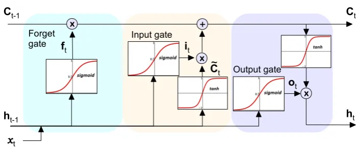
Figure 1.4–A Long Short-Term Memory (LSTM) Cell at time stept

there is a need for tight conditions on eigenvalues of the recurrent matrix during training.

Long Short-Term Memory (LSTM)

LSTM (Hochreiter and Schmidhuber, 1997) networks are extensions of RNNs that reduce the effects of vanishing and exploding gradients. They used gating mech-anism to control memory cells, instead of hidden units from sigmoid or tanh, where the gating is a way to optionally let information through and composed of asigmoidlayer and point-wise multiplication operation. The cells transport infor-mation through units and gates allow the flow of inforinfor-mation to hidden neurons as well as remember information from previous step (i.e., remove or add informa-tion to the cell state). As a result, LSTMs propagate errors for much longer than ordinary RNNs and therefore, can exploit long range dependencies in the data.

In principle, an LSTM4 _{(Hochreiter and Schmidhuber, 1997) creates a self} loop path from where gradient can flow and the self loop corresponds to an eigen-value of Jacobian to be slightly less5 _{than 1, such that} _∂_newState_/∂_oldState _≈ Identity.

LSTM Formulation: Figure 1.4 illustrates an LSTM cell at time stept that

consists of three gates: Forget, Input and Output. We discus the mechanics below:

1. The forget gate ft using sigmoid layer decides what information to keep

or throw away from the previous cell state Ct−1. It takes in the input xt

of current time step t and hidden state ht−1 of previous step, and outputs

4_{www.iro.umontreal.ca/˜bengioy/talks/DL-Tutorial-NIPS2015.pdf}

5_{If an eigenvalue of Jacobian is} _{1, the gradients explode. If an eigenvalue of Jacobian}

is1, the gradients vanish. See Gupta (2019) orwww.dbs.ifi.lmu.de/Lehre/DLAI/

(38)

a number between 0 and 1 corresponding to each number in the cell state

Ct−1. Therefore, it learns weights to control information decay.

f_t=sigmoid(W_xfx_t+W_hfh_t₋₁+b_f) (1.7)

2. On other hand, the input gatei_t selectively updates the cell state C_t based

on the new input, where thesigmoidlayer decides which values to update. Additionally, A tanh layer creates candidate values _C˜

t to be selected to

include to the cell state. Next,i_tandC˜_tare combined to updateC_t.

it=sigmoid(Wxixt+Whiht−1+bi) ˜

C_t=tanh(W_xgx_t+W_hgh_t₋₁+b_g) (1.8)

3. The old cell stateC_t₋₁ is now updated into a new oneC_tas:

C_t=f_t_∗C_t₋₁+i_t_∗C˜_t (1.9)

4. Finally, the output gate ot takes in the current input xt, previous hidden

stateh_t₋₁and current cell stateC_t, and regulates the amount of information

from the cell stateCtthat goes into hidden stateht. ot =sigmoid(Wxoxt+Whoht−1+bo)

ht =ot∗tanh(Ct)

(1.10)

Limitations of LSTMs: Though LSTMs have been successful in modeling sequential data, they suffer from higher memory requirements due to an increase (4 times) in the number of parameters compared to a simple RNN. There is even a higher computational complexity due to multiple memory cells introduced in LSTMs.

Gated Recurrent Unit (GRU)

Like the LSTM, a GRU (Chung et al., 2014) deals with the vanishing gradient problem in RNNs via gating mechanism. It combines the forget and input gates of LSTM into a single update gate. Moreover, the cell state and hidden states are merged into a single memory content. In a way, the GRU does not have a controlled exposure of the memory content to other units in the network. It is different to LSTM due to an output gate with a controlled exposure. Though, the resulting GRU model is simpler than a standard LSTM, it has shown competitive performance and gained popularity.

(39)

Input Layer x1 x2 xE

o1 o2... oC

...

W_ho

Hidden Layer Output

Layer

x1 x2 ... xE h1 h2 ... hH

h1 h2 ... hH

W_xh

x1 x2 ... xE x1 x2 ... xE h1 h2 ... hH

W_hhL _W_hhR Hidden Layer

Output Layer

Internal Nodes

hL(η) hR(η)

W_xh W_xh

W_xh

h(η)

x

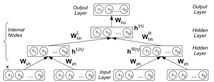
Figure 1.5 – A Recursive Neural Network (RecvNN) architecture. Here, η

indicates a current node,L(η)andR(η)are the left and right children ofηin

the tree structure. The leaf nodes consist of word vectorsx_∈RE.

1.2.2 Recursive Neural Network (RecvNN)

A Recursive Neural Network (Goller and K¨uchler, 1996; Socher et al., 2011b, 2013), a generalization of Recurrent Neural Network operates on a structured in-put, i.e., tree structure instead of a sequence. RecvNN expects a fixed number of branches within a tree structure and recursively computes parent representations in a bottom-up fashion, by combining child nodes. The computation is sequen-tially calculated from the leaf nodes toward the root node.

Recursive Neural Network Formulation: Figure 1.5 demonstrates an ar-chitecture of TreeRNN that operates on binary tree structure with word vector (x_∈RE) representations at the leaves and hidden vectorshas internal nodes. For

a current nodeη, the hidden (internal) vectorh(η)of a current nodeηis computed

from the hidden vectors (hL(η) and hR(η)) of its left L(η) and right R(η) child

nodes, as:

h(η) =fH(WL(η)hL(η)+WR(η)hR(η)+b) (1.11)

where fH is an activation function (e.g., sigmoid, tanh, etc.) for hidden layer.

Notice that whenη is a leaf node then, hL(η) = xL(η), hR(η) = xR(η), WL(η) =

WL_xh, WR(η) = W_xhR andb = bl ∈ RE. Here, x∈ RE is an input word vector.

On other hand, when η is not a leaf node then, WL(η) = W_hhL , WR(η) = W_hhR

andb = b_h _∈ RH. Here, the weights WL_xh andW_xhR connect a leaf (e.g., word

embedding) to its hidden vectors, whereasW_hhL andWR_xh are the weight matrices

that connect hidden vectors of left and right children respectively to the parent vector representation. The vectorsb_handb_lare biases for hidden and input layers,

(40)

Θ

S1 S2

GΘ(S1) GΘ(S2)

Neural

Network Neural Network

Distance

metric

d

(h1,h2)

y

weights shared

h₁ h₂

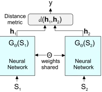
Figure 1.6–A Siamese Neural Network architecture.

Based on the task, an output layer can be attached to each of the hidden vectors in the tree structure to perform a classification for the nodeη.

o(η) =fo(Wohh(η)+bo) (1.12)

Here, fo is an activation function (e.g., sigmoid or softmax) for output layer in

case of classification task. In Figure 1.5, a output layer is attached to the root only, suggesting a sentence-level classification task.

One of the keybenefitsof such topological composition order is that RecvNNs can express relationships between long-distance elements compared to RNNs, be-cause the depth is logarithmic inN if the element count is N. Thus, they have

been applied to scene parsing (Socher et al., 2011b), sentiment analysis (Socher et al., 2013), paraphrase detection (Socher et al., 2011a), dependency parsing (Kiperwasser and Goldberg, 2016), relation extraction (Liu et al., 2015b; Miwa and Bansal, 2016; Zhang et al., 2018), etc.

Our Contribution: In the realm of relation extraction within and across sen-tence boundary, we present a novel inter-sentential Dependency-based Neural Network(iDepNN) (Gupta et al., 2019c) that essentially combines the recurrent and recursive networks over dependency parse features to extract long-distant re-lationships between entities, spanning sentence boundary.

1.2.3 Siamese Neural Network (SNN)

(41)

the twin network is symmetric in the sense that whenever we present two distinct inputs (e.g., image or text pairs), the top conjoining layer will compute the same metric as if we were to present the same two inputs but to the opposite twins.

When applied to textual pairs, the aim of training is to learn text pair repre-sentations to form a highly structured space, where they reflect complex semantic relationships.

Siamese Neural Network Formulation: Figure 1.6 illustrates a Siamese ar-chitecture, where a neural network, e.g., RNN, LSTM, CNN, etc. can be applied to each of the two branches. The aim of the neural networks is to find a function

GΘ that can generate feature representations and map input into a target space,

such that a distance metricd in the target space approximates the “semantic”

dis-tance in the input space. In doing so, the learning is performed by finding theθ

(being shared) that minimizes a loss function, evaluated over a training set. AssumeS1andS2 are two input sentence andGΘis a feature generator (e.g.,

RNN, LSTM, CNN, etc.) within a neural network framework. The twin network shares Θand generates h1 and h2 mapped in a features space from each of the

branches, where the distance functiond is small ifS1 andS2 belong to the same

category or similar, and large otherwise.ymeasures the compatibility betweenS1

andS2, i.e., a category in case of classification or a similarity/dissimilarity score.

Several mapping function GΘ have been investigated. Turk and Pentland

(1991) applied a PCA-based method and Yang et al. (2000) outlined non-linear extensions using Kernel-PCA and Kernel-LDA. Further, Chopra et al. (2005) em-ployed CNN-based feature generators in an application to face verification. To assess semantic similarity between sentences, Mueller and Thyagarajan (2016) and Yin et al. (2016) applied LSTM and CNN networks to encode the underlying meaning expressed in sentence pairs.

Our Contribution: We present a Siamese-based neural architecture, which we named as Replicated Siamese(Gupta et al., 2018a), applied to an industrial ticketing system to learn similarity in textual pairs beyond sentences.

1.3 Unsupervised Neural Density Estimators

(42)

RBM

(Hinton, 2002) RSM (Ruslan and Hinton, 2009)

NADE

(Larochelle and Murray, 2002)

DeepNADE

(Uria et. al., 2014)

DocNADE

(Larochelle and Lauly, 2012)

Deep DocNADE

(Zheng et.al., 2012)

RNN-RSM

(Gupta et. al, 2018)

iDocNADEe

(Gupta et. al, 2019)

iDeepDNEe

(Gupta et. al, 2019)

ctx-DocNADEe

(textTOvec) (Gupta et. al, 2019)

Figure 1.7–RBM and NADE evolution with our contributions

of explanatory factors captured in such generative models is measured by their predictive data-likelihood in the sense that the probability density function of the model is as close as possible to the data distribution.

In the following section, we discuss several probability density estimators, especially Restricted Boltzmann Machine (RBM) (Smolensky, 1986) and its ex-tensions in an unsupervised neural network setting. Table 1.3 defines the notations used in describing the different density estimators.

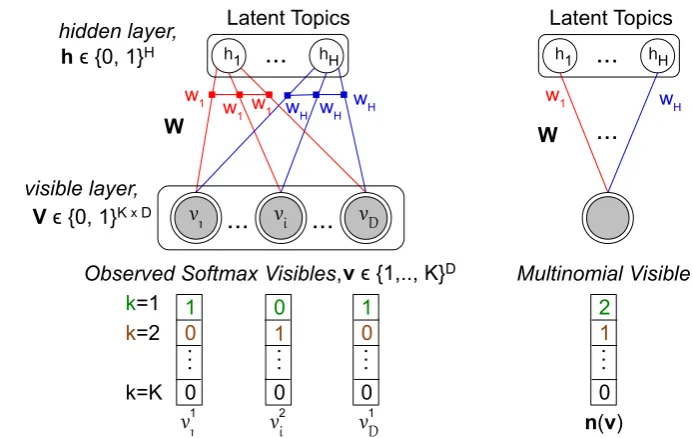
Our Contribution(s): Figure 1.7 summarizes the evolution of neural density estimators, as discussed in the context of this dissertation. It includes the density estimators of binary as well as count (i.e., text) data, where the four rightmost rectangular boxes (i.e.,RNN-RSM, iDocNADEe, iDeepDNEeandctx-DocNADEe) signify our research contributions in the realm of document topic modeling.

1.3.1 Restricted Boltzmann Machine (RBM)

Restricted Boltzmann Machine (Smolensky, 1986; Freund and Haussler, 1992; Hinton, 2002) is a type of two-layer neural network, consisting of stochastic units with undirected interactions between pairs of observed visible (input)V and

un-observed hidden Hunits. The visible and hidden units (or neurons) are binary,

which can be seen as being arranged in two layers. The visible units form the first layer and represent the observable data (e.g., one visible unit for each pixel of a digital input image). The hidden units model dependencies between the com-ponents of observations (e.g., dependencies between pixels in images) and are inferred from the visible units.

(43)

Notation Data Type Description

v _{0,1_}D _{Binary visible units}

h RH _{Hidden units}

V {0,1}K×D _{An observed binary matrix in}_RSM

K I Vocabulary size

N I Number of documents in a corpus

D I Number of visible units; document size inDocNADE

H I Number of units (i.e., dimension) in a hidden layer

Z R Partition function

E R Energy of the model

E - Expectation

b RD Visible bias

c RH Hidden bias

W RD×H _{Weights connecting visible-to-hidden layers in}_RBM_and_NADE

W0 _RH×D _{Weights connecting hidden-to-visible layer in}_NADE

W RH×K Weights connecting visible-to-hidden layers inRSMandDocNADE

U RK×H Weights connecting hidden-to-visible layers inDocNADE

Θ _{} A set of parameters

bold+lowercase - A vector

bold+uppercase - A matrix

Table 1.3–Notations used in the unsupervised density estimators

backward passes between hidden and visible layers, such that the probability dis-tribution represented by the RBM fits the training data.

The RBM is a special type of Boltzmann Machine (BM) (Ackley et al., 1985) without lateral connections where the pair interactions Iare restrictedto be

be-tween visible and hidden units, i.e., I = _{{i, j_} : i _∈ v, j _∈ h_}. Each unit (or

neuron) can take one of the two states, i.e., either 0 or 1, where the joint state of all the units is defined by an associated energy. Figure 1.8 provides graphical illustrations of a BM and an RBM.

RBMs belong to Energy Based Models (EBMs) (Hopfield, 1982) that cap-ture dependencies between observed and unobserved units through modifying an energy function determined by the pair interactions of visible and hidden states, weights and biases. A high energy configuration/state implies a bad compatibil-ity in configuration/pairwise interactions of the units. Therefore, an RBM learning corresponds to minimizing a predefined energy function, and the states of the units are updated in a stochastic manner.

(44)

v

1

v

D

v

i

h

1

h

j

h

H

v

1

v

i

v

D

h

1

h

j

h

H

A Boltzmann Machine (BM) A Restricted Boltzmann Machine (RBM)

... ...

hidden layer,

visible layer,

W

v ϵ {0, 1}D

h ϵ {0, 1}H

Figure 1.8–(left) A Boltzmann Machine (BM), where the dashed lines indi-cate visible-visible or hidden-hidden connections. (right) A Restricted Boltz-mann Machine (RBM), an undirected graphical model based on a bipar-tite graph with the pair connections between visible and hidden units, while visible-visible and hidden-hidden connections (dashed lines in BM) are not al-lowed (i.e., restricted). Each visible (or hidden) unit is arranged into a visible (or hidden) layer and therefore, an RBM is seen as a 2-layered neural network with symmetric connections viaWin visible-visible and hidden-hidden units.

Formulation of an RBM

In a binary RBM of D visible units v = (v1, ..., vD) and n hidden units h =

(h1, ..., hH), the random variables (v,h) take values (v,h)∈ {0,1}D+H and the

joint probability distributionp(v,h)under the model is related to an energy

func-tionE(v,h)and is given by:

p(v,h) = 1

Z exp(−E(v,h)) (1.13)

whereZ is the partition function (normalization constant):

Z =X

v

X

h

exp(₋E(v,h)) (1.14)

and the energy functionE(v,h) takes the following form in order to model the

relationship between the visible and hidden variables:

E(v,h) =₋bTv₋cTh₋vTWh (1.15)

whereW _∈ RD×H is the weight matrix connecting hidden and visible units, and bandcare biases of the visible and hidden layers, respectively.

Intractability: We can observe that the partition functionZ is computed by

(45)

Factorial Distributions via Conditionals: Due to the bipartite graph6 struc-ture of RBMs, the visible and hidden units are conditionally independent given one-another, i.e., its conditional distributionsp(v_|h)andp(h_|v)are factorial and

tractable, i.e, easy to compute.

Given the joint distribution (equation 1.13) and associated energy function (equation 1.15), the conditional distribution on the visible unitsvis computed as:

p(h_|v) = p(v,h)

p(v)

= 1

p(v) 1

Z exp(b

T_v₊_cT_h₊_vT_Wh₎

= 1

Z0 exp(c

T_h₊_vT_Wh₎

= 1

Z0 exp(

H

X

j=1

cjhj+ H

X

j=1

vTW:,jhj)

= 1

Z0

H

Y

j=1

exp(cjhj+vTW:,jhj)

(1.16)

Due to the factorial nature of the conditionals, we can write the joint prob-ability over the vector h as the product of (unnormalized) distributions over the

individual elements,hj:

p(h_|v) = H

Y

j=1

p(hj|v) (1.17)

p(v_|h) = D

Y

i=1

p(vi|h) (1.18)

Here, each unitiorjis turned ON with probabilityp(vi = 1|h)orp(hj = 1|v)

and turned OFF with probability 1₋p(vi = 1|h) or1−p(hj = 1|v). In other

words, an RBM tries to find an optimal configuration in the network via paired visible-hidden connections such as positively paired connections seek to share the same state (i.e., be both ON or OFF), while the negatively paired connections prefer to be in different states.

6_{a graph whose vertices can be divided into two disjoint and independent sets such that no two}

(46)

Now, normalizing the distributions over individual binaryhj as:

p(hj = 1|v) =

p(hj = 1|v)

p(hj = 0|v) +p(hj = 1|v)

= exp(cj +v

T_W

:,j) exp(0) + exp(cj+vTW:,j) =sigmoid(cj+vTW:,j)

(1.19)

Therefore, the full conditional over the hidden layer is expressed as the facto-rial distribution:

p(h_|v) = H

Y

j=1

sigmoid(cj+vTW:,j) (1.20)

Similarly, the conditional distribution on the hidden unitshis given by:

p(v_|h) = 1

Z00

D

Y

i=1

exp(bivi+viWi,:h) (1.21)

and the full conditional over the visible layer is expressed as the factorial distribu-tion:

p(v_|h) = D

Y

i=1

sigmoid(bi+Wi,:h) (1.22)

Due to the factorial nature of the conditionals, one can efficiently draw sam-ples from the joint distribution via a block Gibbs sampling7_{strategy (Casella and} George, 1992). For instance, each iteration of block Gibbs sampling (Markov chain) consists of two steps: (1): Sampleh(l)_∼p(h_|v(l))and (2): Samplev(l+1) ∼p(v_|h(l)). We can simultaneously and independently sample from all the

ele-ments ofh(l)givenv(l)andv(l+1) givenh(l), respectively.

Training Restricted Boltzmann Machines

During training, an RBM learns to reconstruct the data in an unsupervised fashion and therefore, iteratively makes several forward and backward passes between the visible and hidden layer to adjust its parameters. In the reconstruction phase, the distance (measured by Kullback-Leibler Divergence) between its estimated probability distribution and the ground-truth distribution of the input is minimized,

7_{The idea is to generate posterior samples by sweeping through each variable (or block of}

variables) to sample from its conditional distribution with the remaining variables fixed to their

current values. Further details: https://ermongroup.github.io/cs323-notes/