Using Occupancy Models to Estimate Temporal and Spatial Variation in Seabird Distributions.

FLANDERS, NICHOLAS P. Using Occupancy Models to Estimate Temporal and Spatial Variation in Seabird Distributions. (Under the direction of Beth Gardner).

Comparisons of seabird distributions across time and space are of interest to ecologists. However, without formally accounting for the imperfect at-sea detection of seabirds, such comparisons are likely to contain bias due to variation in detection probability. Distance sampling methodology is an attractive analysis option but is not applicable when data is collected under strip-transect survey protocols. We analyzed aerial strip-transect survey data collected in southern New England using community occupancy models and dynamic occupancy models to make comparisons across space and time while formally accounting for imperfect detection probabilities. Predictions of species-specific winter distributions were made in two study plots, one off the coast of Rhode Island and the other in Nantucket Sound, using environmental covariate relationship estimates from two

ensured easy interpretability of these results for decision-makers.

by

Nicholas P. Flanders

A thesis submitted to the Graduate Faculty of North Carolina State University

in partial fulfillment of the requirements for the degree of

Master of Science

Fisheries, Wildlife, and Conservation Biology

Raleigh, North Carolina 2014

APPROVED BY:

______________________ _____________________ Beth Gardner Allan O’Connell

Committee Chair

DEDICATION

BIOGRAPHY

ACKNOWLEDGEMENTS

TABLE OF CONTENTS

LIST OF TABLES ... vi

LIST OF FIGURES ... vii

USING A COMMUNITY OCCUPANCY MODEL TO IDENTIFY KEY SEABIRD AREAS IN SOUTHERN NEW ENGLAND ... 1

ABSTRACT ... 1

INTRODUCTION ... 2

METHODS ... 3

Study area ... 3

Aerial strip-transect surveys ... 4

Environmental covariates ... 5

Model description ... 6

Implementation ... 9

Making predictions and comparisons ... 10

RESULTS ... 11

DISCUSSION ... 14

Environmental covariate relationships and predicted distributions ... 15

Improving models for predicting seabird distributions ... 17

Conservation implications ... 19

LITERATURE CITED ... 20

APPENDIX ... 32

USING DYNAMIC OCCUPANCY MODELS TO INVESTIGATE INTER-ANNUAL SHIFTS IN SEABIRD DISTRIBUTIONS IN SOUTHERN NEW ENGLAND ... 71

ABSTRACT ... 71

INTRODUCTION ... 72

METHODS ... 73

Study site ... 73

Aerial strip-transect surveys ... 74

Environmental covariates ... 74

Dynamic occupancy model ... 75

Implementation and model selection ... 77

Making predictions ... 77

RESULTS ... 78

DISCUSSION ... 80

LITERATURE CITED ... 84

LIST OF TABLES

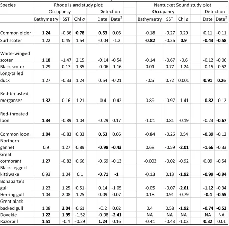
Using a Community Occupancy Model to Identify Key Seabird Areas in Southern New England Table 1. Effects of environmental covariates on occupancy and detection probabilities of seabirds included in both winter models. Posterior means of species-specific coefficients are shown, with significant coefficient estimates indicated in bold. Dovekie was not included in the Nantucket Sound model but is shown here because some species-specific covariate effects were significant.

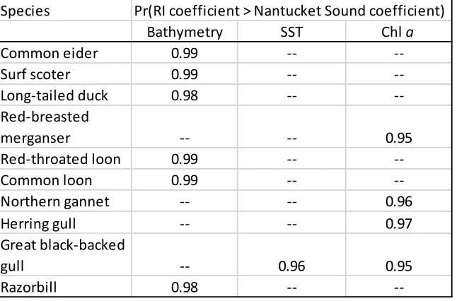
... 25 Table 2. Significant probabilities of differences between Rhode Island study plot and Nantucket Sound study plot estimates of relationships between covariates and occupancy in winter. ... 26

Using Dynamic Occupancy Model to Investigate Inter-annual Shifts in Seabird Distributions in Southern New England

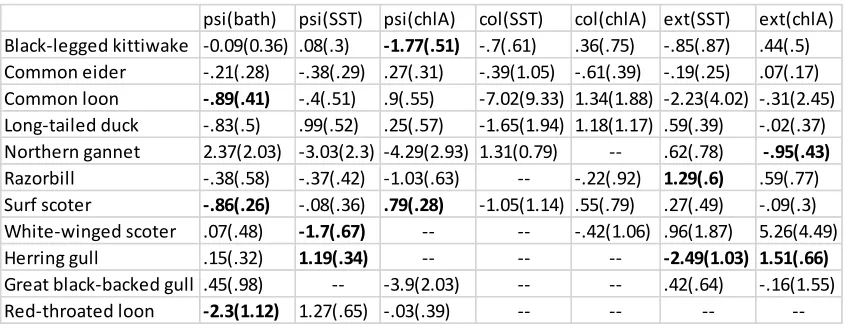
Table 1. Model-averaged estimates of species-specific relationships between bathymetry (bath), sea surface temperature (SST), and chlorophyll a surface concentration (chlA) and initial occupancy (psi), colonization (col), and extinction (ext). Bold indicates significant estimate; coefficients not

LIST OF FIGURES

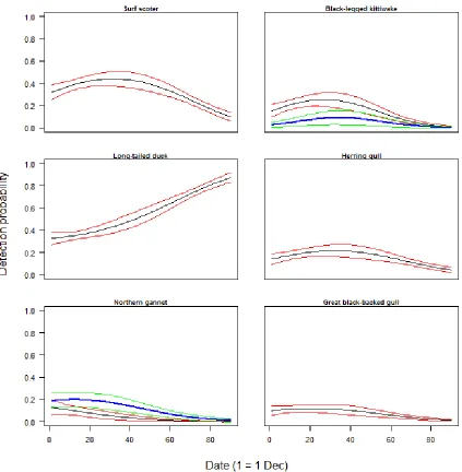
Using a Community Occupancy Model to Identify Key Seabird Areas in Southern New England Figure 1. Map of Nantucket Sound study plot, aerial survey transect lines, and bathymetry raster. ... 27 Figure 2. Means and 95% credible intervals of predicted detection probabilities across winter season dates for species with significant linear and quadratic effects of date on 𝑝. Black and red lines for Nantucket Sound study plot winter 2003-2004, blue and green lines for Rhode Island study plot winter 2009-2010. ... 28 Figure 3. Map of the posterior means of predicted winter occupancy for selected diving species; A: common eider, B: common loon, C: northern gannet, D: razorbill. ... 29 Figure 4. Map of the posterior means of predicted winter occupancy for selected surface-feeding species; A: black-legged kittiwake, B: herring gull. ... 30 Figure 5. Map of the posterior means of the predicted number of species in the observed communities for the winter season. ... 31

Using Dynamic Occupancy Model to Investigate Inter-annual Shifts in Seabird Distributions in Southern New England

Figure 1. Map of Nantucket Sound study plot, aerial survey transect lines, and bathymetry raster. ... 88 Figure 2. Predicted occupancy probabilities of white-winged scoter, surf scoter, and black-legged kittiwake across Nantucket Sound study plot in winter 2003-2004, winter 2004-2005, and winter 2005-2006. ... 89

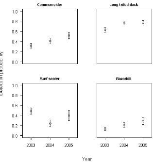
Figure 3. Year-specific detection probability intercept estimates for common eider, long-tailed duck, surf scoter, and razorbill in winter 2003-2004, winter 2004-2005, and winter 2005-2006.

USING A COMMUNITY OCCUPANCY MODEL TO IDENTIFY KEY SEABIRD AREAS IN SOUTHERN NEW ENGLAND

ABSTRACT

Estimating the relationships between seabird distributions and environmental variables is a common goal in seabird studies. When distance data is not recorded, researchers may have difficulty estimating detection probability, which is known to vary by species. However, repeated sampling of aerial strip-transects and occupancy models can be used to account for species-specific detection rates less than one. To our knowledge, this approach has not been previously used to estimate seabird distributions. We applied single-season community occupancy models to datasets collected in two large study plots in southern New England. We estimated the influence of

remotely-sensed environmental covariates including bathymetry, sea surface temperature, and chlorophyll a surface concentration on species-specific occupancy. Similarly, we modeled detection as a function of both survey date and effort. The two study plots were modeled separately to explore differences in predicted distributions and species-specific environmental covariate

relationships. Diving species showed large differences between the two study plots in terms of their predicted winter distributions, which was largely explained by bathymetry acting as a stronger predictor of occupancy in Rhode Island than in Nantucket Sound. Conversely, similarities between the two study plots in predicted winter distributions of surface-feeding species were explained by sea surface temperature or chlorophyll a concentration acting as predictors of these species’

INTRODUCTION

Determining relationships between seabird distributions and environmental variables is

Community occupancy models (Dorazio & Royle 2005) offer an alternative approach for the analysis of aerial seabird survey data, provided there is temporal replication of strip transect surveys within a period during which some form of geographical closure can be assumed . These models do not estimate abundance, but instead the probability of site-occupancy by a species, and information is lost when reducing counts to binary detection/non-detection data (MacKenzie et al. 2002, 2006). However, community occupancy models account for the imperfect detection of species and allow for inference about species-specific habitat relationships and predicted distributions for species that are rare or difficult to detect (Russell et al. 2009, Ruiz-Gutiérrez et al. 2010). Community-level metrics such as species richness can also be estimated (Dorazio et al. 2006, Royle et al. 2007, Zipkin et al. 2009, 2010b). Traditional distance sampling techniques assume perfect detection at distance 0 from the transect (Buckland et al. 2001). Community occupancy models do not make this

assumption and allow for the probability of a species being available for detection to be less than one (Tyre et al. 2003, MacKenzie 2005, MacKenzie et al. 2006, Kéry & Schaub 2012).

Here, we applied community occupancy models to estimate relationships between seabird

occupancy and a suite of environmental covariates to predict areas of high seabird occupancy across two study plots in the northwestern Atlantic Ocean. We expect these results to increase our

knowledge of seabird ecology and distribution in the region, thereby supporting those responsible for decisions regarding ocean planning.

METHODS Study area

Winiarski et al. 2014). The Rhode Island study plot encompassed the boundaries of the Rhode Island Ocean Special Area Management Plan (RIOSAMP; Winiarski et al. 2011). The other study plot was located in Massachusetts, USA, and included much of Nantucket Sound (Fig. 1). Both study plots provide important habitat for a diversity of seabird species (Huettmann & Diamond 2000), including the federally-endangered roseate tern (Sterna dougallii) and species of conservation concern such as the common loon (Gavia immer), red-throated loon (Gavia stellata), least tern (Sterna

antillarum), and great shearwater (Puffinus gravis; Kinlan et al. 2012a, Winiarski et al. 2013). The study area is also globally important for wintering sea ducks (Tribe Mergini; Caithamer et al. 2000, Zipkin et al. 2010a, Silverman et al. 2013).

Aerial strip-transect surveys

Sound surveys used strips that were 91-m wide on each side of the plane and no ancillary information on glare was recorded.

For both study plots, transect lines were divided into 2.27-km long sections to form unique segments. The length of the southernmost segment of most transects in the Nantucket Sound study plot was variable due to different transect lengths; these variable segments had a mean length of 1065 m (SD = 640). All avian observations used in this analysis were identified to species and given the appropriate segment identification as an attribute. We defined the winter season as the months of December-February and selected the winter 2003-2004 data from the Nantucket Sound study plot to form two single-season datasets, where most segments had within-season temporal replication. Data were segregated by species and survey-specific counts were reduced to binary data to represent the detection or non-detection of a species within each segment.

Environmental covariates

1/3 arc-second resolution bathymetry digital elevation model (DEM) of Nantucket Sound from NOAA (Eakins et al. 2009). These grids were overlaid spatially with the transect segments and weighted average covariate values for each segment were calculated (Zipkin et al. 2010a). This raster processing was accomplished using Spatial Analyst Tools in ArcMap10 (ESRI 2011).

Based on the data collected for the survey locations, the distribution of bathymetry values in the Rhode Island study plot covered a larger range of values and the overall mean was deeper than in the Nantucket Sound study plot (Fig. 1). Ranges of SST and chl a concentration values were similar between the two study plots for both seasons (Appendix Sec. 1.1). The mean of the SST values was slightly greater in the Rhode Island study plot, whereas the chl a concentration values from the Nantucket Sound study plot had a greater mean than the Rhode Island study plot.

Model description

For each single-season model, we assumed that a survey segment was either occupied or not by a given species over the course of the sampling season. The latent state 𝑧𝑖𝑘 represents this process, as 𝑧𝑖𝑘 = 1 if segment 𝑖 is occupied by species 𝑘 and 𝑧𝑖𝑘 = 0 if segment 𝑖 is not occupied by species 𝑘(MacKenzie et al. 2002, 2006). These binary latent states were modeled as Bernoulli random

variables with success probability Ψ, which represents the occupancy probability.

The segment-level covariate values were standardized by subtracting from the mean and dividing by the standard deviation. We then used a logit link to model Ψ as a function of bathymetry and seasonal averages of both SST and chl a concentration (chlA) at the segment level (Kéry & Royle 2008a, 2008b, Russell et al. 2009) such that

𝑙𝑜𝑔𝑖𝑡(Ψ𝑖𝑘) = 𝑜𝑐𝑐𝑖𝑛𝑡𝑘+ 𝛽1,𝑘𝑏𝑎𝑡ℎ𝑦𝑚𝑒𝑡𝑟𝑦𝑖+ 𝛽2,𝑘𝑆𝑆𝑇𝑖+ 𝛽3,𝑘𝑐ℎ𝑙𝐴𝑖

We assumed that the season-specific data came from an imperfect observation process, with 𝑦_𝑖𝑗𝑘 = 1 if species 𝑘 is observed at site 𝑖 during survey occasion 𝑗 and 𝑦𝑖𝑗𝑘 = 0 if species 𝑘 is not

observed at site 𝑖 during survey occasion 𝑗 (MacKenzie et al. 2002, 2006). We also assumed that there were no false positives (or misidentification errors), thus a positive detection means that the site was occupied by the species during the survey season. However, the outcome 𝑦𝑖𝑗𝑘 = 0 could

arise from two scenarios: either site 𝑖 is not occupied by species 𝑘 during the survey season or site 𝑖 is occupied but the observer failed to detect species 𝑘 during survey occasion 𝑗. The temporal replication of surveys at segments closed to changes in occupancy by a species enabled us to estimate the detection probability. Detection probability, 𝑝, is defined as the success probability of a random Bernoulli process that generates 𝑦𝑖𝑗𝑘, given that site 𝑖 is occupied by species 𝑘 during the

survey season. Specifically, 𝑦𝑖𝑗𝑘|𝑧𝑖𝑘 ~ 𝐵𝑒𝑟𝑛( 𝑝𝑖𝑗𝑘∗ 𝑧𝑖𝑘); thus, when 𝑧𝑖𝑘 = 0 the probability of a detection is 0 and when 𝑧𝑖𝑘 = 1 the probability of a detection is 𝑝𝑖𝑗𝑘.

We modeled variation in 𝑝 as a function of date and observer effort (Kéry & Royle 2008a, 2008b, Russell et al. 2009). Differences in estimates of observer effort collected under the two sampling protocols for the study areas led to the construction of two different observation sub-models. Both sub-models estimated both linear and quadratic effects of date on 𝑝, as we expected a temporal trend in detection probability across a survey period due to intra-seasonal changes in abundance (Kendall 1999, MacKenzie et al. 2003, Royle & Nichols 2003, Zipkin et al. 2009, Gardner et al. 2011). For the Rhode Island data, we accounted for reduced observer effort at survey locations with significant glare by including an indicator variable 𝑔𝑙𝑎𝑟𝑒𝑖𝑗= 0 when only one observer was recording data and 𝑔𝑙𝑎𝑟𝑒𝑖𝑗= 1 at normal double observer survey occasions such that

where 𝑝𝑖𝑛𝑡1,𝑘 is the intercept for species 𝑘 with glare (only one observer on survey) and 𝑝𝑖𝑛𝑡2,𝑘 is the intercept for species 𝑘 when there is no glare effect (both observers on survey).

Nantucket Sound survey flights through a given segment showed significant variation in length. Therefore, we modeled 𝑝 as a function of survey length when analyzing these data such that

𝑙𝑜𝑔𝑖𝑡(𝑝𝑖𝑗𝑘) = 𝑝𝑖𝑛𝑡𝑘+ 𝛼1,𝑘𝑑𝑎𝑡𝑒𝑖𝑗+ 𝛼2,𝑘𝑑𝑎𝑡𝑒𝑖𝑗2+ 𝛼3,𝑘𝑙𝑒𝑛𝑔𝑡ℎ𝑖𝑗

where 𝑝𝑖𝑛𝑡𝑘 is the species-specific intercept.

To broaden the scope of our inference about the seabird ecology of the study areas, we adopted the community occupancy modeling approach of Dorazio & Royle (2005). This approach has been used to increase the precision of estimates for rare species and for testing hypotheses about habitat relationships at the community level (Russell et al. 2009; Zipkin et al. 2009, 2010b; Ruiz-Gutiérrez et al. 2010). Kéry & Royle (2008b) showed the flexibility of this approach when incorporating

covariates on the species-specific sub-models of the hierarchical framework.

Our community occupancy models assumed that each of the species-specific parameters was a random effect arising from a Normal prior distribution (Sauer & Link 2002, Dorazio & Royle 2005, Royle & Dorazio 2006):

𝛽_1,𝑘~𝑁𝑜𝑟𝑚𝑎𝑙(𝜇_𝛽1, 𝜎_𝛽2₁₎

Due to the nature of this study, we adopted a different interpretation of the occupancy parameter to allow for more flexibility in meeting the closure assumption of occupancy models. Typically, effective detection probability is defined as the probability of detecting a species given that the site is occupied by the species and the species is available for detection at the site (Kendall 1999, Tyre et al. 2003, MacKenzie 2005, MacKenzie et al. 2006, Kéry & Schaub 2012, Johnson et al. 2014). This interpretation of 𝑝 means that a species’ detection probability is confounded with the species’ probability of availability (Gray et al. 2013, Johnson et al. 2014). This effective detection probability is reduced compared to the traditional detection probability where a probability of availability equal to 1 is assumed (Kendall 1999, Russell et al. 2009, Gray et al. 2013). Instead of the probability of permanent site occupancy by a species, we interpreted Ψ as the probability of site usage by the species during the study period (MacKenzie 2005, MacKenzie et al. 2006, Kéry & Schaub 2012). If we assume that the process driving the availability of the species, movement on and off of the site, is temporary and random (Burnham 1993, Kendall et al. 1997), we can avoid bias in our estimates despite the lack of strict closure (Kendall 1999, MacKenzie 2005, MacKenzie et al. 2006, Kéry & Schaub 2012). As this effective detection probability is reduced relative to traditional detection probability, the precision of estimates can be expected to decrease accordingly (Kendall 1999). Implementation

significant if their 95% credible intervals did not overlap zero. Convergence of all parameters was reached as determined by R-hat values (Gelman & Hill 2007) and visual inspection of trace plots. Making predictions and comparisons

We used grids with 4-km2 _{(2 x 2 km) cells for spatial predictions of occupancy probability across} the two study plots. Spatial Analyst Tools in ArcMap10 (ESRI 2011) were used to obtain weighted average seasonal covariate values for each grid cell; these grid cell-level values were standardized with the original covariate means and standard deviations used in the analysis. To map means and standard deviations of the number of observed species predicted to occupy each grid cell, we included new 𝑧𝑖k parameters for each grid cell 𝑖 and for each species 𝑘 observed in the respective study plot. These 𝑧𝑖k parameters were modeled as Bernoulli random variables with success

probability equal to the occupancy probability predicted at the respective grid cell for the respective species and were summed across species at each iteration to approximate the posterior distribution of the grid cell-specific predictions.

We compared seabird habitat relationships between the Nantucket Sound and Rhode Island study plots by calculating the probability that the season and species-specific coefficient estimates for a given habitat relationship differed between the two study plots for a given species. These probabilities were calculated following Ruiz-Gutiérrez et al. (2010). We considered there was a significant difference between species-specific estimates from the two study plots if the probability of this difference was ≥ 0.95.

feed primarily at or near the ocean surface (Appendix Sec. 1.3). These foraging guilds were not used during the modeling process but rather for qualifying consistent relationships across species with similar natural history.

RESULTS

Surveys of the Rhode Island study plot conducted during the 2009-2010 winter season detected 17 species (Appendix Sec. 1.4), 13 of which were diving species and four of which were surface-feeding species. Species-specific estimates of the relationship between bathymetry andoccupancy were significant for eight species, all of which were diving species. The great black-backed gull (Larus marinus), a surface-feeding species, and dovekie (Alle alle), a diving species, were the only species with significant relationships between SST and occupancy. Common eider (Somateria mollissima), a diving species, was the only species with a significant relationship between chl a and occupancy (Table 1). Five species had significant estimates for the relationship between date and detection, and three species had significant estimates for the quadratic effect of date on detection (Table 1, Fig. 2).

Bathymetry was the strongest predictor of the distributions of diving species in the Rhode Island study plot in the winter (Table 1), which is not surprising as foraging sea ducks and some other diving species are typically associated with shallow depths (Guillemette et al. 1993, Nehls &

were surface-feeding species. The only species with a significant relationship between bathymetry and its occupancy was surf scoter (Melanitta perspicillata), a diving species. There were no

significant species-specific estimates of the relationship between SST and occupancy in this model. Species-specific estimates of the relationship between chl a concentration and occupancy were significant for five species, three of which were surface-feeding species (Table 1). Ten species had significant estimates for the relationship between date and detection, and six species had significant estimates for the quadratic effect of date on detection (Table 1, Fig. 2).

We found a significant difference in our estimates of species-specific relationships between bathymetry and occupancy from the two study plots for six species, all of which were diving species. The great black-backed gull was the only species for which we found a significant difference in the parameter estimates for SST from the two study plots. We found a significant difference in the estimates of species-specific relationships between chl a concentration and occupancy from the two study plots for red-breasted merganser (Mergus serrator), a diving species, and for three surface-feeding species: herring gull (Larus argentatus), northern gannet (Morus bassanus), and great black-backed gull (Table 2).

Predicted distributions across the Rhode Island study plot for diving piscivores such as red-throated loon, common loon (Fig. 3), red-breasted merganser, and great cormorant (Phalacrocorax carbo) were similar to those for sea ducks, with areas of high predicted occupancy occurring near the mainland and near islands (Appendix Sec. 2). No consistent pattern in predicted occupancy for these diving piscivore species was evident in the Nantucket Sound study plot. The predicted distribution of northern gannet, another diving piscivore, in the Rhode Island study plot included areas of high occupancy across most of the study plot, with a patchier pattern of high occupancy predicted in the Nantucket Sound study plot (Fig. 3).

Patterns of predicted occupancy were much more similar between the two study plots for black-legged kittiwake (Rissa tridactyla) and herring gull (Fig. 4), which is representative of our findings for other surface-feeding species included in both winter models (Appendix Sec. 2). In both study plots, areas of high predicted occupancy were large and concentrated away from the mainland. The razorbill (Alca torda) was the only alcid included in both winter models and predicted distributions were similar to those of the sea ducks (Fig. 3). In contrast, dovekie was only detected in the Rhode Island study plot and its predicted distribution was strongly concentrated in the south-central portion of the study plot (Appendix Sec. 2).

Detection probability was modeled as a quadratic function of date to account for changes in species abundance across the two three-month seasons. Species-specific detection probabilities were expected to reach a maximum when the species was at peak abundance in the study plot. Thus, it is interesting that the predicted detection of long-tailed duck in the Nantucket Sound study plot reached its maximum at the end of the winter season, while the maximum predicted detection of northern gannet in the Rhode Island and Nantucket Sound study plots occurred at the beginning of the winter season (Fig. 2).

DISCUSSION

We used community occupancy models to draw inference on habitat relationships for seasonal seabird communities that included uncommon species with few detections. This approach appears suitable for analyzing data from aerial seabird surveys that include temporal and spatial replication, as our model results largely agreed with both our a priori expectations and findings from other analyses in southern New England (Winiarski et al. 2013, 2014). We found considerable variation among species in estimates of relationships between occupancy and environmental covariates, much of which concurred with our a priori placement of species into two foraging guilds.

Comparisons of parameter estimates and predicted distributions for the same species also showed considerable differences between the two study plots. This finding confirms that species-specific habitat relationships and distributions can be area-specific and extrapolating patterns from one area to another, even if areas are close geographically, may prove problematic. Regulators making offshore development decisions must use predicted seabird distributions that are based on survey data from the area in question.

assumed (MacKenzie et al. 2002, Tyre et al. 2003). The two species with significant estimates of both linear and quadratic effects of date on detection in both winter models, northern gannet and black-legged kittiwake, showed significantly different detection probability estimates between the two study plots for some portion of the winter season. By allowing detection probability to vary among both species and study plots we avoided potential confounding of ecological parameter differences with differences in detection rate (Kéry et al. 2008, Ruiz-Gutiérrez et al. 2010).

Environmental covariate relationships and predicted seabird distributions

Primary productivity tends to be concentrated in certain areas of the ocean, usually related to levels of nutrient enrichment (Kinlan et al. 2012b). These areas tend to concentrate seabird prey and provide important habitat for foraging seabirds (Hyrenbach et al. 2000, Spear et al. 2001, Ballance et al. 2006, Louzao et al. 2006, Bost et al. 2009, Louzao et al. 2009). Sea surface temperature and chl a concentration can be used as indices for primary productivity and prey density near the surface of the ocean; thus we expected these covariates to be significant predictors of the distributions of surface-feeding species. However, diving piscivores present in the study region were able to forage at a variety of depths in the water column, and a number of surface water characteristics could predict foraging habitat for these species as well (Harrison 1983, Winiarski et al. 2013).

winter surface-feeding species’ occupancy in Nantucket Sound. This result was not a surprise, although it was a notable departure from patterns in results from the Rhode Island model. Differences and similarities in patterns of predicted occupancy for the two study plots can be explained by species-specific covariate relationship estimates from the two models. Large differences in predicted distributions of winter diving species can be explained by bathymetry showing up as a much stronger predictor of species’ occupancy in the Rhode Island study plot than in the Nantucket Sound study plot. Predicted winter distributions of surface-feeding species are more similar between the two study plots. This can be explained by either SST or chl a

concentration showing up as strong predictors of species’ occupancy in both study plots.

Specifically, the covariate relationship driving these species’ distributions in the Rhode Island model shows a positive effect for SST, whereas the relationship driving these species’ distributions in the Nantucket Sound model is a negative effect of chl a concentration. At the level of spatial resolution we used winter values of SST and chl a concentration appear negatively correlated in the study region.

It was surprising to see significant negative relationships between chl a concentration and surface-feeding species’ occupancy in the Nantucket Sound model as chl a concentration is believed to be a proxy for primary productivity and thus prey density (Hyrenbach et al. 2002). However, the spatial resolution of the covariate data may have been too coarse to allow the model to detect associations between seabird occupancy and small patches of primary productivity represented by high local chl a concentration values (Huettmann & Diamond 2006). Instead, extensive variation in chl a

instead be an artifact of these species’ distributions being concentrated farther from the mainland. Similarly, the significantly positive relationships between chl a concentration and the winter

occupancy of some sea ducks are likely a result of winter chl a concentration values at this level of spatial resolution serving as an effective proxy of distance to shore rather than a proxy of local prey patches, as these sea ducks are associated with benthic, sessile prey in shallow and near-shore areas (Guillemette et al. 1993). Nevertheless, these coefficients are useful for predicting patterns of occupancy of these species across the two study plots.

Our spatial predictions of the number of observed species occupying grid cells across the two study plots are directly relevant to conservation efforts in the region. The pattern of this metric across the Rhode Island study plot resembles the general spatial pattern of predicted occupancy for diving species in this plot, while the pattern of this metric across the Nantucket Sound study plot resembles the spatial pattern of predicted occupancy for surface-feeding species (Fig. 6). It appears that the predicted occupancy of diving species is driving the spatial distribution of this metric in the Rhode Island study plot and the predicted occupancy of surface-feeding species is driving such patterns in the Nantucket Sound study plot. The usefulness of such a metric may increase by weighting species differently based on species-specific levels of conservation concern (Winiarski et al. 2014).

Improving models for predicting seabird distributions

The analysis of temporally-replicated aerial seabird survey data with occupancy models is an improvement over other distribution modeling techniques, such as those using presence-only data, that do not formally account for imperfect detection probabilities (Yackulic et al. 2013). We note that occupancy models require several assumptions, including the spatial independence of

a dynamic ocean landscape could lead to violations of this assumption if the same individuals are detected at multiple sites during a given survey flight. Efforts are taken to reduce double counting of individuals and incorporation of spatially explicit covariates may reduce the impacts of this

correlation. Occupancy models also assume that no false positives, or misidentification errors, occur (MacKenzie et al. 2002, Tyre et al. 2003, MacKenzie 2005, Kéry & Royle 2008a, Kéry & Schaub 2012). Large seabird datasets collected by aerial surveys are likely to contain some errors as it can be difficult to identify individuals under such challenging conditions. In using 2.27-km long segments and reducing survey counts to binary data, our goal was to minimize the effect of misidentification and false positives in our analyses.

Conservation implications

LITERATURE CITED

Bailey LL, Reid JA, Forsman ED, Nichols JD (2009) Modeling co-occurrence of northern spotted and barred owls: accounting for detection probability differences. Biol Conserv 142:2983-2989

Ballance LT, Pitman RL, Fiedler PC (2006) Oceanographic influences on seabirds and cetaceans of the eastern tropical Pacific: a review. Prog Oceanogr 69:360-390

Bost CA, Cotté C, Bailleul F, Cherel Y, Charrassin JB, Guinet C, Ainley DG, Weimerskirch H (2009) The importance of oceanographic fronts to marine birds and mammals of the southern oceans. J Marine Syst 78:363-376

Buckland ST, Anderson DR, Burnham KP, Laake JL, Borchers DL, Thomas L (2001) Introduction to Distance sampling: estimating abundance of biological populations. Oxford University Press, London

Burnham KP (1993) A theory for combined analysis of ring recovery and recapture data. In: Lebreton JD, North PM (eds) Marked individuals in the study of bird population. Birkhäuser-Verlag, Basel, Switzerland, p 199-214

Caithamer DF, Otto M, Padding PI, Sauer JR, Haas GH (2000) Sea ducks in the Atlantic flyway: population status and a review of the special hunting seasons. US Fish and Wildlife Service, Laurel, MD

Camphuysen CJ, Fox AD, Leopold M, Petersen IK (2004) Towards standardised seabirds at sea census techniques in connection with environmental impact assessments for offshore wind farms in the UK. In: UK COWRIE 1 Report. Royal Netherlands Institute for Sea Research, Texel, Netherlands Dorazio RM, Royle JA (2005) Estimating size and composition of biological communities by modeling the occurrence of species. J Am Stat Assoc 100:389-398

Dorazio RM, Royle JA, Söderström B, Glimskär A (2006) Estimating species richness and accumulation by modeling species occurrence and detectability. Ecology 87:842-854

Drewitt AL, Langston RHW (2006) Assessing the impacts of wind farms on birds. Ibis 148:29-42 Eakins BW, Taylor LA, Carignan KS, Warnken RR, Lim E, Medley PR (2009) Digital elevation model of Nantucket, Massachusetts: procedures, data sources, and analysis. NOAA Technical Memorandum NESDIS NGDC-26, Dept. of Commerce, Boulder, CO

Gardner B, Gilbert AT, O’Connell AF (2011) Compendium of avian occurrence information for the continental shelf waters along the Atlantic coast of the United States (modeling section – seabird distributions). A final report for the U.S. Department of the Interior, Minerals Management Service, Atlantic OCS Region, Herndon, VA, in prep.

Gelman A, Hill J (2007) Data analysis using regression and multilevel/hierarchical models. Cambridge University Press, New York, NY

GEODAS Grid Translator-Design-a-Grid (2006)

http://www.ngdc.noaa.gov/mgg/gdas/gd_designagrid.html

Gray BR, Holland MD, Yi F, Starcevich LAH (2013) Influences of availability on parameter estimates from site occupancy models with application to submersed aquatic vegetation. Nat Resour Model 26:526-545

Guillemette M, Himmelman JH, Barette C, Reed A (1993) Habitat selection by common eiders in winter and its interaction with flock size. Can J Zoolog 71:1259-1266

Harrison P (1983) Seabirds: an identification guide. Houghton Mifflin Company, New York, NY Hedley SL, Buckland ST (2004) Spatial models for line transect sampling. J Agric Biol Environ Stat 9:181-199

Huettmann F, Diamond AW (2000) Seabird migration in the Canadian North Atlantic: moulting locations and movement patterns of immature birds. Canadian J Zoolog 78:624-647

Huettmann F, Diamond A (2006) Large-scale effects on the spatial distribution of seabirds in the Northwest Atlantic. Landscape Ecol 21:1089–1108

Hyrenbach KD, Fernández P, Anderson DJ (2002) Oceanographic habitats of two sympatric North Pacific albatrosses during the breeding season. Mar Ecol Prog Ser 233:283-301

Hyrenbach KD, Forney KA, Dayton PK (2000) Marine protected areas and ocean basin management. Aquatic Conserv: Mar Freshw Ecosyst 10:437-458

Johnson FA, Dorazio RM, Castellón TD, Martin J, Garcia JO, Nicholas JD (2014) Tailoring point counts for inference about avian density: dealing with nondetection and availability. Nat Resour Model 27:163-177

Kendall WL, Nichols JD, Hines JE (1997) Estimating temporary emigration using capture-recapture data with Pollock’s robust design. Ecology 78:563-578

Kéry M, Royle JA (2008a) Hierarchical Bayes estimation of species richness and occupancy in spatially replicated surveys. J Appl Ecol 45:589-598

Kéry M, Royle JA (2008b) Inference about species richness and community structure using species- specific occupancy models in the National Swiss Breeding Bird Survey MHB. In: Thomson DL, Cooch EG, Conroy MJ (eds) Modeling demographic processes in marked populations. Springer, New York, NY, p 639-656

Kéry M, Royle JA, Schmid H (2008) Importance of sampling design and analysis in animal population studies: a comment on Sergio et al. J Appl Ecol 45:981-986

Kéry M, Schaub M (2012) Bayesian population analysis using WinBUGS. Elsevier, Boston

Kinlan BP, Menza C, Huettmann F (2012a) Chapter 6: predictive modeling of seabird distribution patterns in the New York Bight. In: Menza C, Kinlan BP, Dorfman DS, Poti M, Caldow C (eds) A biogeographic assessment of seabirds, deep sea corals and ocean habitats of the New York Bight: science to support offshore spatial planning. NOAA Technical Memorandum NOS NCCOS 141, Silver Spring, MD, p 87-224

Kinlan BP, Poti M, Menza C (2012b) Chapter 4: oceanographic setting. In: Menza C, Kinlan BP, Dorfman DS, Poti M, Caldow C (eds) A biogeographic assessment of seabirds, deep sea corals and ocean habitats of the New York Bight: science to support offshore spatial planning. NOAA

Technical Memorandum NOS NCCOS 141 Silver Spring, MD, p 59-68

Langston, RHW (2013) Birds and wind projects across the pond: a UK perspective. Wildlife Soc B 37:5-18

Louzao M, Becares J, Rodriguez B, Hyrenbach KD, Ruiz A, Arcos JM (2009) Combining vessel-based surveys and tracking data to identify key marine areas for seabirds. Mar Ecol Prog Ser 391:183– 197

Louzao M, Hyrenbach K, Arcos J, Abelló P, de Sola L, Oro D (2006) Oceanographic habitat of an endangered Mediterranean procellariiform: implications for marine protected areas. Ecol Appl 16:1683–1695

MacKenzie DI (2005) Was it there? Dealing with imperfect detection for species presence/absence data. Aust N Z J Stat 47:65-74

MacKenzie DI, Nichols JD, Lachman GB, Droege S, Royle JA, Langtimm CA (2002) Estimating site occupancy rates when detection probabilities are less than one. Ecology 83:2248-2255

MacKenzie DI, Nichols JD, Royle JA, Pollock KH, Bailey LL, Hines JE (2006) Occupancy estimation and modeling. Elsevier, UK

Nehls G, Ketzenberg C (2002) Do common eiders Somateria mollissima exhaust their food resources? A study on natural mussel Mytilus edulis beds in the Wadden Sea. Danish Review of Game Biology 16:47-61

Nur N, Jahncke J, Herzog MP, Howar J, Hyrenbach KD, Zamon JE, Ainley DG, Wiens JA, Morgan K, Ballance LT, Stralberg D (2011) Where the wild things are: predicting hotspots of seabird

aggregations in the California current system. Ecol Appl 21:2241–2257

Petersen IB, MacKenzie M, Rexstad E, Wisz MS, Fox AD (2011) Comparing pre- and post-construction distributions of long-tailed ducks Clangula hyemalis in and around the Nysted offshore wind farm, Denmark: a quasi-designed experiment accounting for imperfect detection, local surface features and autocorrelation. CREEM Tech Report 2011-1, St. Andrews, Scotland

Plummer M (2011) JAGS version 3.3.0 manual. http://sourceforge.net/projects/mcmc-jags/ R Development Core Team (2011) R: A language and environment for statistical computing. R Foundation for Statistical Computing, Vienna, Austria

Roberts JJ, Best BD, Dunn DC, Treml EA, Halpin PN (2010) Marine Geospatial Ecology Tools: an integrated framework for ecological geoprocessing with ArcGIS, Python, R, MATLAB, and C++. Environ Modell Softw 25:1197-1207

Royle JA, Dorazio RM (2006) Hierarchical models of animal abundance and occurrence. J Agr Biol Envir St 11:249-263

Royle JA, Dorazio RM, Link WA (2007) Analysis of multinomial models with unknown index using data augmentation. J Comput Graph Stat 16:67-85

Royle JA, Nichols JD (2003) Estimating abundance from repeated presence absence data or point counts. Ecology 84:777-790

Sauer JR, Link WA (2002) Hierarchical modeling of population stability and species group attributes from survey data. Ecology 86:1743-1751

Schneider DC (1997) Habitat selection by marine birds in relation to water depth. Ibis 139:175-178 Silverman ED, Saalfeld DT, Leirness JB, Koneff MD (2013) Wintering sea duck distribution along the Atlantic coast of the United States. Journal of Fish and Wildlife Management 4:178-198

Spear LB, Balance LT, Ainley DG (2001) Response of seabirds to thermal boundaries in the tropical Pacific: the thermocline versus the Equatorial Front. Mar Ecol Prog Ser 219:275-289

Tremblay Y, Bertrand S, Henry RW, Kappes MA, Costa DP, Shaffer SA (2009) Analytical approaches to investigating seabird-environment interactions: a review. Mar Ecol Prog Ser 391:153-163

Tyre AJ, Tenhumberg B, Field SA, Niejalke D, Parris K, Possingham HP (2003) Improving precision and reducing bias in biological surveys: estimating false-negative error rates. Ecol Appl 13:1790-1801 Winiarski KJ, Miller DL, Paton PWC, McWilliams SR (2013) Spatially explicit model of wintering common loons: conservation implications. Mar Ecol Prog Ser 492:273-283

Winiarski KJ, Miller DL, Paton PWC, McWilliams SR (2014) A spatial conservation prioritization approach for protecting marine birds given proposed offshore wind energy development. Biol Con 169:79-88

Winiarski KJ, Paton P, Trocki CL, McWilliams SR (2011) Spatial distribution, abundance, and flight ecology of birds in nearshore and offshore waters of Rhode Island: January 2009 to August 2010. Rhode Island Ocean Special Area Management Plan Interim Report, Kingston, Rhode Island Yackulic CB, Chandler R, Zipkin EF, Royle JA, Nicholas JD, Campbell Grant EH, Veran S (2013)

Presence-only modelling using MAXENT: when can we trust the inferences? Methods in Ecology and Evolution 4:236-243

Zipkin EF, DeWan A, Royle JA (2009) Impacts of forest fragmentation on species richness: a hierarchical approach to community modeling. J Appl Ecol 46:815-822

Zipkin EF, Gardner B, Gilbert AT, O’Connell Jr. AF, Royle JA, Silverman ED (2010a) Distribution patterns of wintering sea ducks in relation to the North Atlantic Oscillation and local

environmental characteristics. Oecologia 163:893-902

Table 1. Effects of environmental covariates on occupancy and detection probabilities of seabirds included in both winter models. Posterior means of species-specific coefficients are shown, with significant coefficient estimates indicated in bold. Dovekie was not included in the Nantucket Sound model but is shown here because some species-specific covariate effects were significant.

Species

Bathymetry SST Chl a Date Date2 Bathymetry SST Chl a Date Date2

Common eider 1.24 -0.36 0.78 0.53 0.06 -0.18 -0.27 0.29 0.11 -0.11

Surf scoter 1.22 0.45 1.54 -0.04 -1.2 -0.82 -0.26 0.9 -0.43 -0.58

White-winged

scoter 1.18 -1.47 2.15 -0.14 -0.54 -0.14 -0.67 -0.6 -0.12 -0.06

Black scoter 1.29 0.17 1.35 -0.06 -1.16 0.01 0.77 -1.24 -0.15 -0.52

Long-tailed

duck 1.27 -0.33 1.24 0.54 -0.21 -0.5 0.72 0.001 0.91 0.26

Red-breasted

merganser 1.32 0.16 1.21 0.4 -0.42 0.89 -0.97 -1.41 -0.82 -0.12

Red-throated

loon 1.34 -0.89 1.04 -0.29 0.17 -1.01 0.81 -0.19 -0.23 -0.67

Common loon 1.04 -0.83 0.33 0.53 0.06 -0.84 -0.26 0.54 -0.39 -0.12

Northern

gannet 0.9 1.27 0.89 -0.98 -0.43 0.68 -0.59 -2.01 -1.66 -0.33

Great

cormorant 1.27 -0.82 0.66 -0.69 -0.13 -0.003 -0.02 -0.92 0.09 -0.54

Black-legged

kittiwake 0.93 1.04 0.1 -0.71 -1 -0.13 0.13 -1.92 -0.99 -0.94

Bonaparte's

gull 1.23 1.25 0.51 0.14 -1.05 -0.05 -0.07 -2.61 -1.12 -0.34

Herring gull 1.04 2.08 1.25 0.09 0.07 0.18 0.91 -0.79 -0.4 -0.55

Great

black-backed gull 1.08 3.04 0.61 -0.2 0.02 0.4 0.58 -1.92 -0.74 -0.52

Dovekie 1.22 1.95 -1.52 -0.08 -2.41 NA NA NA NA NA

Razorbill 1.51 -0.4 -0.29 1.24 0.16 -0.41 -0.43 -1.02 0.32 0.01

Detection Occupancy

Nantucket Sound study plot

Occupancy Detection

Table 2. Significant probabilities of differences between Rhode Island study plot and Nantucket Sound study plot estimates of relationships between covariates and occupancy in winter.

Species

Bathymetry SST Chl a

Common eider 0.99 --

--Surf scoter 0.99 --

--Long-tailed duck 0.98 --

--Red-breasted

merganser -- -- 0.95

Red-throated loon 0.99 --

--Common loon 0.99 --

--Northern gannet -- -- 0.96

Herring gull -- -- 0.97

Great black-backed

gull -- 0.96 0.95

Razorbill 0.98 --

Figure 3. Map of the posterior means of predicted winter occupancy for selected diving species; A: common eider, B: common loon, C: northern gannet, D: razorbill.

A

_B

Figure 4. Map of the posterior means of predicted winter occupancy for selected surface-feeding species; A: black-legged kittiwake, B: herring gull.

Figure 5. Map of the posterior means of the predicted number of species in the observed communities for the winter season.

Sec. 1.1. Comparison of means and ranges of covariate values used for seasonal analysis of Rhode Island Ocean SAMP (RIOSAMP) and Nantucket Sound datasets. RIOSAMP data from winter 2009-2010 and Nantucket Sound data from winter 2003-2004.

Sec. 1.2. Example BUGS code for community occupancy model sink("commmodel15.txt")

cat(" model { # Priors

for(k in 1:(nspec)){

lpsi[k] ~ dnorm(mu.lpsi, tau.lpsi)

betalpsi1[k] ~ dnorm(mu.betalpsi1, tau.betalpsi1) betalpsi2[k] ~ dnorm(mu.betalpsi2, tau.betalpsi2) betalpsi3[k] ~ dnorm(mu.betalpsi3, tau.betalpsi3)

lp[k] ~ dnorm(mu.lp, tau.lp)

betalp1[k] ~ dnorm(mu.betalp1, tau.betalp1) betalp2[k] ~ dnorm(mu.betalp2, tau.betalp2) betalp3[k] ~ dnorm(mu.betalp3, tau.betalp3) }

mu.lpsi ~ dnorm(0,0.01) tau.lpsi <- pow(sd.lpsi, -2) sd.lpsi ~ dunif(0,20)

mu.betalpsi1 ~ dnorm(0,0.01) tau.betalpsi1 <- pow(sd.betalpsi1, -2) sd.betalpsi1 ~ dunif(0,20)

mu.betalpsi2 ~ dnorm(0,0.01) tau.betalpsi2 <- pow(sd.betalpsi2, -2)

Mean (SD) Range

RIOSAMP -35.44 (8.50) (-55.86, -10.33) Nantucket Sound -11.53 (3.27) (-19.32, -0.92)

Bathymetry

Mean (SD) Range Mean (SD) Range

RIOSAMP 5.79 (0.58) (4.23, 6.73) 2.96 (0.51) (1.88, 5.60) Nantucket Sound 3.28 (0.23) (2.66, 4.12) 4.88 (0.58) (3.57, 7.44)

sd.betalpsi2 ~ dunif(0,20) mu.betalpsi3 ~ dnorm(0,0.01) tau.betalpsi3 <- pow(sd.betalpsi3, -2) sd.betalpsi3 ~ dunif(0,20)

mu.lp ~ dnorm(0,0.01) tau.lp <- pow(sd.lp, -2) sd.lp ~ dunif(0,20)

mu.betalp1 ~ dnorm(0,0.01) tau.betalp1 <- pow(sd.betalp1, -2) sd.betalp1 ~ dunif(0,20)

mu.betalp2 ~ dnorm(0,0.01) tau.betalp2 <- pow(sd.betalp2, -2) sd.betalp2 ~ dunif(0,20)

mu.betalp3 ~ dnorm(0,0.01) tau.betalp3 <- pow(sd.betalp3, -2) sd.betalp3 ~ dunif(0,20)

# Likelihood for(k in 1:(nspec)){ for (i in 1:nsite) {

psi[i,k] <- exp(lpsi[k] + betalpsi1[k] * bath[i] + betalpsi2[k] * SST[i] + betalpsi3[k] * chla[i])/(1+exp(lpsi[k] + betalpsi1[k] * bath[i] + betalpsi2[k] * SST[i] + betalpsi3[k] * chla[i])) z[i,k] ~ dbern(psi[i,k])

} }

for(k in 1:(nspec)){ for (i in 1:nsite){ for(j in 1:J[i]){

p[i,j,k] <- exp(lp[k] + betalp1[k] * date[i,j] + betalp2[k] * pow(date[i,j],2) + betalp3[k] *

leng[i,j])/(1+exp(lp[k] + betalp1[k] * date[i,j] + betalp2[k] * pow(date[i,j],2) + betalp3[k] * leng[i,j])) p.eff[i,j,k] <- z[i,k] * p[i,j,k]

Y[i,j,k] ~ dbern(p.eff[i,j,k]) }

} }

predocc[j,k]<-exp(lpsi[k] + betalpsi1[k] * bathpred[j] + betalpsi2[k] * SSTpred[j] + betalpsi3[k] * chlapred[j])/(1+exp(lpsi[k] + betalpsi1[k] * bathpred[j] + betalpsi2[k] * SSTpred[j] + betalpsi3[k] * chlapred[j]))

newz[j,k] ~ dbern(predocc[j,k]) }

}

for(j in 1:npredsite){

predspecies[j]<-sum(newz[j,1:nspec]) }

}

",fill = TRUE) sink()

Sec. 1.3. Classification of species included in models based on foraging method Winter

Diving species Surface-feeding species

common eider (Somateria mollissima) brant (Branta bernicla)

surf scoter (Melanitta perspicillata) black-legged kittiwake (Rissa tridactyla) white-winged scoter (Melanitta fusca) bonaparte's gull (Chroicocephalus philadelphia)

black scoter (Melanitta americana) herring gull (Larus argentatus) long-tailed duck (Clangula hyemalis) great black-backed gull (Larus marinus) red-breasted merganser (Mergus serrator)

red-throated loon (Gavia stellata) common loon (Gavia immer) red-necked grebe (Podiceps grisegena)

northern gannet (Morus bassanus) great cormorant (Phalacrocorax carbo)

dovekie (Alle alle) common murre (Uria aalge)

Sec. 1.4. Detected species and number of detections at the segment level, Rhode Island Ocean SAMP study plot winter 2009-2010

Sec. 1.5. Detected species and number of detections at the segment level, Nantucket Sound study plot winter 2003-2004

Species Number of detections

common eider (Somateria mollissima) 44

surf scoter (Melanitta perspicillata) 1

white-winged scoter (Melanitta fusca) 10

black scoter (Melanitta americana) 1

long-tailed duck (Clangula hyemalis) 1

red-breasted merganser (Mergus serrator) 2

red-throated loon (Gavia stellata) 15

common loon (Gavia immer) 232

northern gannet (Morus bassanus) 105

great cormorant (Phalacrocorax carbo) 2

black-legged kittiwake (Rissa tridactyla) 47

bonaparte's gull (Chroicocephalus philadelphia) 1

herring gull (Larus argentatus) 152

great black-backed gull (Larus marinus) 92

dovekie (Alle alle) 24

common murre (Uria aalge) 1

razorbill (Alca torda) 11

Species Number of detections

brant (Branta bernicla) 1

common eider (Somateria mollissima) 463

surf scoter (Melanitta perspicillata) 365

white-winged scoter (Melanitta fusca) 146

black scoter (Melanitta americana) 21

long-tailed duck (Clangula hyemalis) 779

red-breasted merganser (Mergus serrator) 12

red-throated loon (Gavia stellata) 38

common loon (Gavia immer) 57

red-necked grebe (Podiceps grisegena) 1

northern gannet (Morus bassanus) 51

great cormorant (Phalacrocorax carbo) 1

black-legged kittiwake (Rissa tridactyla) 147

bonaparte's gull (Chroicocephalus philadelphia) 21

herring gull (Larus argentatus) 183

great black-backed gull (Larus marinus) 93

Sec. 2.5. Posterior means of predicted white-winged scoter occupancy, winter.

USING DYNAMIC OCCUPANCY MODELS TO INVESTIGATE INTER-ANNUAL SHIFTS IN SEABIRD DISTRIBUTIONS IN SOUTHERN NEW ENGLAND

ABSTRACT

Inter-annual variation must be taken into account when studying seabird distributions, with important areas, or “hotspots,” for diving species expected to be more persistent across time than those for surface-feeding species. We avoided confounding seabird distribution dynamics with changes in year-specific detection rates by analyzing a three-year winter-season aerial seabird survey dataset from southern New England using dynamic occupancy models. We allowed for spatial variation in probabilities of site-occupancy, extinction, and colonization using the environmental covariates bathymetry, sea surface temperature, and chlorophyll a surface

INTRODUCTION

Given the dynamic nature of seabird habitat (Louzao et al. 2006, 2009; Kinlan et al. 2012) it is important to consider inter-annual variability when investigating seabird distributions. The

distribution of foraging seabirds is a result of individual habitat selection choices made in a manner that maximizes predatory efficiency (Kirk et al. 2008, Stephens 1986). Thus, the distribution of wintering seabirds in the northwestern Atlantic Ocean is largely dictated by the availability of prey. Prey of sea ducks and other seabirds that forage by diving to considerable depths below the ocean surface are often sessile with distributions tied to bathymetry (Guillemette et al. 1993, Schneider 1997, Bost et al. 2009, Kinlan et al. 2012). Prey of surface-feeding species (Flanders et al. in review) often have distributions associated with more ephemeral features (Hyrenbach et al. 2000). Thus, we expected less inter-annual variation in distributions of diving species than those of surface-feeding species (Louzao et al. 2006, Zipkin et al. 2010, Silverman et al. 2013).

observers’ skill level, or logistical details of surveys (MacKenzie et al. 2003, Ruiz-Gutiérrez et al. 2010). Occupancy modeling is a method used to account for imperfect detection when strip-transect seabird surveys include both spatial and temporal replication (Flanders et al. in review). Dynamic occupancy models extend analyses to data from multiple years collected under a robust design (Pollock 1982, MacKenzie et al. 2003). These models estimate initial occupancy rates as well as probabilities of site colonization and extinction, all of which can be allowed to vary spatially using covariates (MacKenzie et al. 2003). By formally accounting for detection, researchers can provide accurate, easily-interpretable information on seabird distribution dynamics.

Here, we applied dynamic occupancy models to estimate seabird distributions in three

consecutive winter seasons across a study site in the northwestern Atlantic Ocean. We accounted for imperfect detection and made predictions at spatial scales relevant to offshore planning. Our results should provide information on species-specific inter-annual variation in distribution that is easily interpreted by decision-makers evaluating the long-term stability of predicted seabird hotspots.

METHODS Study site

Aerial strip-transect surveys

The Massachusetts Audubon Society collected data using aerial surveys flown at an altitude of 152 m over 15 transect lines within Nantucket Sound (Fig. 1). For details on data collection protocols see Flanders et al. (in review). The survey data selected for this analysis came from the winter 2003-2004, winter 2004-2005, and winter 2005-2006 seasons, with the winter season defined as the months of December-February. We chose only the winter season in each year as closure-related assumptions of occupancy models were expected to be more easily satisfied than in spring or fall and summer data were scarce and likely affected by breeding colony locations. Most segments had within-season temporal replication in all three years, with a maximum number of 9 surveys at a segment in winter 2003-2004, 6 in winter 2004-2005, and 3 in winter 2005-2006.

Environmental covariates

Dynamic occupancy model

We exploited the temporal and spatial replication inherent to the Nantucket Sound survey design and analyzed the data with single-species dynamic occupancy models (MacKenzie et al. 2003). We assumed that each segment was either occupied or not by a given species over the course of each winter season. The latent state 𝑧𝑖𝑡represents this process, as 𝑧𝑖𝑡 = 1 if segment 𝑖 is occupied during season 𝑡 and 𝑧𝑖𝑡 = 0 if segment 𝑖 is not occupied during season 𝑡 (MacKenzie et al. 2002, MacKenzie et al. 2006). These binary latent states were modeled as Bernoulli random variables with success probability Ψ𝑡, which represents the occupancy probability during season 𝑡. In our sub-model for initial occupancy we used a logit link to model Ψ1, species-specific initial occupancy, as a function of bathymetry and seasonal averages of both SST and chl a concentration (MacKenzie et al. 2003, MacKenzie et al. 2006) such that

𝑙𝑜𝑔𝑖𝑡(Ψ𝑖1) = 𝛼𝑝𝑠𝑖 + 𝛽1𝑏𝑎𝑡ℎ𝑦𝑚𝑒𝑡𝑟𝑦𝑖+ 𝛽2𝑆𝑆𝑇𝑖1+ 𝛽3𝑐ℎ𝑙𝑎𝑖1

where 𝛼𝑝𝑠𝑖is the species-specific intercept.

Dynamic occupancy models allow the occupancy state to change between seasons such that segments unoccupied at time 𝑡 could become colonized at time 𝑡 + 1 with probability 𝛾 and segments occupied at time 𝑡 could go extinct at time 𝑡 + 1 with probability 𝜖 (MacKenzie et al. 2003). We allowed for spatial variation in extinction and colonization probabilities using a logit link and covariates that varied by year (MacKenzie et al. 2003, MacKenzie et al. 2006). In our sub-model for extinction probability we modeled 𝜖 as a function of segment-level averages of SST and chl a such that

where 𝛼𝜖 is the species-specific intercept. Our sub-model for species-specific colonization probability had identical structure to extinction with coefficients for SST and chl a concentration. We chose the variables bathymetry, SST, and chl a concentration as covariates as they are readily available at adequate spatial and temporal scales and are known to be important predictors of seabird distributions (Ballance et al. 2006, Nur et al. 2011, Kinlan et al. 2012). We did not include bathymetry as a covariate on colonization and extinction probabilities as it made more intuitive sense to model these processes as functions of the temporally dynamic covariates SST and chl a concentration.

Dynamic occupancy models assume an imperfect observation process (MacKenzie et al. 2002, 2006). Specifically, 𝑦𝑖𝑗𝑡|𝑧𝑖𝑡 ~ 𝐵𝑒𝑟𝑛(𝑝𝑖𝑗𝑡∗ 𝑧𝑖𝑡); thus, when 𝑧𝑖𝑡 = 0 the probability of a detection is 0

and when 𝑧𝑖𝑡 = 1 the probability of a detection is 𝑝𝑖𝑗𝑡. We allowed 𝑝 to vary by year and as a

function of date and observer effort (MacKenzie et al. 2003). We included both linear and quadratic effects of date on 𝑝, as we expected a temporal trend in detection probability across a survey season due to intra-seasonal changes in abundance (Kendall 1999, MacKenzie et al. 2003, Royle & Nichols 2003, Zipkin et al. 2009, Gardner et al. 2011). The lengths of the Nantucket Sound survey flight tracks through a given segment showed significant variation, so we modeled 𝑝 as a function of survey length such that

𝑙𝑜𝑔𝑖𝑡(𝑝𝑖𝑗𝑡) = 𝑝𝑖𝑛𝑡𝑡+ 𝛼1𝑑𝑎𝑡𝑒𝑖𝑗𝑡+ 𝛼2𝑑𝑎𝑡𝑒𝑖𝑗𝑡2+ 𝛼3𝑙𝑒𝑛𝑔𝑡ℎ𝑖𝑗𝑡

where 𝑝𝑖𝑛𝑡𝑡 is the species and season-specific intercept.

study period (MacKenzie 2005, MacKenzie et al. 2006, Kéry & Schaub 2012). For more details on this interpretation see Flanders et al. (in review).

Implementation and model selection

All dynamic occupancy models were fitted using the R package “unmarked” (Fiske & Chandler 2011). For species with more than fifty detections in at least one winter season (Appendix Sec. 1), we ran the global model described above and then an additional 127 nested models with all possible combinations of covariates on initial occupancy, colonization, and extinction probabilities. We fitted only nine models for species with between thirty and fifty detections in at least one winter season (Appendix Sec. 1). In all cases, we included the global detection probability models as we expected both survey length and survey date to be important predictors of detection for many species (Flanders et al. in review). Convergent models were ranked by Akaike’s Information Criterion (AIC) and parameter estimates were averaged based on models within two delta AIC of the best model (Burnham & Anderson 2002). We used the R package “AICcmodavg” to obtain model-averaged point estimates and standard errors of the parameters (Mazerolle 2013).

Making predictions

We used a grid with 2 km x 2 km cell size resolution for spatial predictions of occupancy

probability in winter 2003-2004, winter 2004-2005, and winter 2005-2006 for each modeled species. Spatial Analyst Tools in ArcMap10 (ESRI 2011) were used to obtain weighted average seasonal covariate values for each grid cell; these grid cell-level values were standardized with the original covariate means and standard deviations used in the analysis. We then used model-averaged estimates and the standardized covariate values to obtain predictions and standard errors of initial occupancy probability for each grid cell. We followed the same procedure to obtain

periods of winter 2003-2004 to winter 2004-2005 and winter 2004-2005 to winter 2005-2006. Predicted occupancy for winter 2004-2005 and winter 2005-2006 was then derived at each grid cell using predicted initial occupancy, colonization, and extinction probabilities as described in

MacKenzie et al. 2003. RESULTS

Ten species had a sufficient number of winter season detections allowing us to run the complete dynamic model set of 128 models (Appendix Sec. 1). We fitted only 9 models for red-throated loon Gavia stellata due to a lower number of detections. Brant (Branta bernicla), black scoter (Melanitta americana), red-breasted merganser (Mergus serrator), red-necked grebe (Podiceps grisegena), great cormorant (Phalacrocorax carbo), and bonaparte’s gull (Chroicocephalus philadelphia) had too few detections to allow any modeling. The number of models that converged for each species was highly variable and complete model selection results for each species are in Appendix Sec. 2. The average of ocean depth values from the study site was 11.56 meters (m) below mean high water (Appendix Sec. 1). The average of SST values from the study site was 3.75 degrees Celsius and the average of chl a concentration values from the study site was 4.25 mg m-3_{. From winter} 2003-2004 to winter 2005-2006 seasonal SST values in the study site increased on average; seasonal winter chl a concentration values in the study plot decreased and then increased again on average over the three years (Appendix Sec. 1).

black-legged kittiwake (Rissa tridactyla) and significantly positive for surf scoter. Model-averaged estimates of the effect of SST on extinction were significantly positive for razorbill (Alca torda) and significantly negative for herring gull, and model-averaged estimates of the effect of chl a on extinction were significantly negative for northern gannet and significantly positive for herring gull. We did not find significant model-averaged estimates of the effects of either SST or chl a on

colonization for any of the modeled species.

Two species, long-tailed duck (Clangula hyemalis) and white-winged scoter, showed little change in their predicted distributions across years (Fig. 2, Appendix Sec. 2). Other species showed dynamics that were relatively constant across the study plot, leaving the spatial configuration of high and low rates of predicted occupancy intact. Common loon, red-throated loon, and surf scoter were three such species that showed overall declines in predicted occupancy across years without significant spatial variation in extinction rate (Fig. 2, Appendix Sec. 2).

All species with significant model-averaged estimates of relationships between covariates and extinction rate showed noticeable spatial variation in predicted occupancy dynamics. The general increase in predicted herring gull and black-legged kittiwake occupancy observed across the study plot showed such spatial variation (Fig. 2, Appendix Sec. 2). Similarly, changes in predicted

occupancy of common eider (Somateria mollissima), razorbill, and great black-backed gull showed spatial variation, but for these species a general decrease in predicted occupancy across the study plot was observed (Appendix Sec. 2). Larger changes were observed for northern gannet, with noticeable increases and decreases in predicted occupancy at varying intensities across the study plot.

black-legged kittiwake and herring gull, had predicted distributions in winter 2003-2004 that included distinct areas of high occupancy in southwestern and eastern portions of the study plot, which disappeared in subsequent winters, as predicted occupancy became uniformly high across the study plot (Fig. 2). An area of relatively low predicted black-legged kittiwake occupancy did remain across years in the northeastern portion of the study plot. Areas of low predicted common eider

occupancy in winter 2003-2004 located in southwestern and eastern portions of the study plot were not present in winter 2004-2005, with an additional area of low predicted occupancy in the

northwestern corner of the study plot appearing in winter 2005-2006. Finally, areas of low predicted northern gannet occupancy in winter 2003-2004 located in the eastern portion of the study plot became areas of high predicted occupancy in subsequent winters.

Most species showed noticeable variation in detection probability among years (Appendix Sec. 2), with significantly different year-specific intercept estimates for four species (Fig. 3). For both razorbill and common eider, estimates of winter 2003-2004 intercepts were lower than in winter 2005-2006. The winter 2003-2004 intercept estimate for long-tailed duck was lower than both winter 2004-2005 and winter 2005-2006 estimates, while the winter 2003-2004 intercept estimate for surf scoter was higher than the 2004-2005 estimate for this species.

DISCUSSION