ABSTRACT
BOBOLEA, NICOLAE ALIN. Thermal Design of Wide Beam Area X-Ray Sources. (Under the direction of Dr. J. Michael Doster.)
Diffraction Enhanced Imaging (DEI) with x-ray radiation provided by a synchrotron source has been shown to provide good image contrast at lower radiation dose for materials with small x-ray attenuation coefficient As a result, DEI has received significant interest for digital mammography and other medical imaging applications. However, deployment of a synchrotron source at a medical facility is not currently feasible due to its size and costs. Consequently, a compact x-ray source capable of delivering x-ray intensities and beam collimation similar to a synchrotron accelerator is desirable.
Thermal Design of Wide Beam Area X-Ray Sources
by
Nicolae Alin Bobolea
A thesis submitted to the Graduate Faculty of North Carolina State University
in partial fulfillment of the requirements for the Degree of
Master of Science
Nuclear Engineering
Raleigh, North Carolina 2009
APPROVED BY:
_________________________________ ________________________________ Dr. Mohamed A. Bourham Dr. K. Linga Murty
DEDICATION
For Ruxandra
BIOGRAPHY
ACKNOWLEDGMENTS
TABLE OF CONTENTS
LIST OF TABLES ... vii
LIST OF FIGURES ... ix
LIST OF SYMBOLS ... xi
LIST OF MATHEMATICAL NOTATIONS ... xiii
Chapter 1 Introduction ... 1
1.1 Wide Beam Area X-ray Sources ... 1
1.2 Simulation using Computational Fluid Dynamics ... 2
Chapter 2 Theory ... 7
2.1 Basic Governing Equations... 8
2.2 Boundary Conditions ... 10
2.3 Turbulence Model ... 12
Chapter 3 Computational Simulation ... 18
3.1 Design Requirements ... 18
3.2 Initial Designs ... 19
3.2.1 Initial Design 01 ... 19
3.2.2 Initial Design 02 ... 27
3.2.3 Initial Design 03 ... 32
3.3 Final Design ... 39
3.3.3 CFD Model ... 49
3.3.4 Evaluation Roadmap ... 51
Chapter 4 Results ... 59
4.1 Uniform Heat Flux Distribution... 59
4.2 Non-uniform Heat Flux Distribution ... 78
4.3 Design Solution Space ... 87
4.4 Result Analysis ... 89
Chapter 5 Conclusions and Future Work ... 97
5.1 Conclusions ... 97
5.2 Future Work ... 98
REFERENCES ... 99
APPENDICES ... 101
Appendix A. Non-Uniform Heat Flux Distribution Maps ... 102
Appendix B. ANSYS CFX-Solver Convergence Plots for Uniform Heat Flux Distribution ... 104
LIST OF TABLES
Table 3.1 – Initial design 01 characteristics ... 20
Table 3.2 – Initial design 01 simulation results (SI units) ... 22
Table 3.3 – Initial design 01 simulation results (British units) ... 23
Table 3.4 – Initial design 02 characteristics ... 28
Table 3.5 – Initial design 02 simulation results (SI units) ... 29
Table 3.6 – Initial design 02 simulation results (British units) ... 30
Table 3.7 – Initial design 03 characteristics ... 34
Table 3.8 – Initial design 03 simulation results (SI units) ... 35
Table 3.9 – Initial design 03 simulation results (British units) ... 35
Table 3.10 – Final design features ... 44
Table 3.11 – Molybdenum properties ... 45
Table 3.12 – Final design mesh characteristics ... 48
Table 3.13 – Model boundary condition details ... 50
Table 4.1 – Final design ver.01 simulation results (SI units) ... 61
Table 4.2 – Final design ver.01 simulation results (British units) ... 63
Table 4.3 – Final design ver.02 simulation results (SI units) ... 65
Table 4.4 – Final design ver.02 simulation results (British units) ... 67
Table 4.5 – Final design ver.03 simulation results (SI units) ... 69
Table 4.8 – Pumping power dependence, W ... 74
Table 4.9 – Normalized maximum target temperature dependence ... 75
Table 4.10 – Normalized pumping power dependence ... 75
Table 4.11 – Final design ver.01 peak to average ratio (SI units) ... 79
Table 4.12 – Final design ver.01 peak to average ratio (British units) ... 80
Table 4.13 – Final design ver.02 peak to average ratio (SI units) ... 81
Table 4.14 – Final design ver.02 peak to average ratio (British units) ... 82
Table 4.15 – Final design ver.03 peak to average ratio (SI units) ... 83
Table 4.16 – Final design ver.03 peak to average ratio (British units) ... 84
Table 4.17 – Peak to average ratio dependence ... 85
LIST OF FIGURES
Figure 3.1 – Initial design 01 geometry ... 21
Figure 3.2 – Flow stagnation and target temperature for inlet velocity 1 m/s ... 24
Figure 3.3 – Velocity and pressure profiles in the radial flow channels ... 25
Figure 3.4 – Initial design 02 geometry ... 27
Figure 3.5 – Initial design 02 results for inlet velocity 3 m/s ... 31
Figure 3.6 – Initial design 03 geometry ... 33
Figure 3.7 – Initial design 03 results for inlet velocity 1 m/s ... 38
Figure 3.8 – Final design geometry – Target front ... 40
Figure 3.9 – Final design geometry – Fins ... 40
Figure 3.10 – Final design geometry – Cooling channels ... 41
Figure 3.11 – Final design geometry – Complete design ... 41
Figure 3.12 – Final design sectional view and highlights ... 43
Figure 3.13 – Final design evaluation roadmap ... 52
Figure 3.14 – Continuous probability density function for normal distribution ... 54
Figure 4.1 – Normalized maximum target temperature dependence ... 76
Figure 4.2 – Normalized pumping power dependence ... 76
Figure 4.3 – Normalized peak to average ratio dependence ... 86
Figure 4.4 – Design solution space ... 88
Figure 4.7 – Peak to average ratio profiler ... 93
Figure 4.8 – Maximum target temperature contour plot ... 94
Figure 4.9 – Pumping power contour plot ... 95
Figure 4.10 – Peak to average ratio contour plot ... 96
Figure A.1 – Non-uniform heat flux distribution for 4.37 peak to average ratio ... 102
Figure A.2 – Non-uniform heat flux distribution for 5.79 peak to average ratio ... 103
Figure A.3 – Non-uniform heat flux distribution for 8.07 peak to average ratio ... 103
Figure B.1 – Mass and momentum convergence plot for final design ver.01 - 0.6 m/s ... 104
Figure B.2 – Heat transfer convergence plot for final design ver.01 - 0.6 m/s ... 105
Figure B.3 – Turbulence convergence plot for final design ver.01 - 0.6 m/s ... 106
Figure C.1 – Uniform heat flux – Heated target area temperature profile ... 107
Figure C.2 – Uniform heat flux – Target temperature profile ... 108
Figure C.3 – Uniform heat flux – Water pressure profile ... 108
Figure C.4 – Uniform heat flux – Water temperature profile ... 109
Figure C.5 – Uniform heat flux – Water velocity streamlines ... 109
Figure C.6 – Uniform heat flux – Water temperature and water velocity profiles ... 110
Figure C.7 – Non-uniform heat flux – Heated target area temperature profile ... 111
Figure C.8 – Non-uniform heat flux – Target temperature profile ... 111
Figure C.9 – Non-uniform heat flux – Water pressure profile ... 112
LIST OF SYMBOLS
This section provides a list of symbols used throughout this thesis together with their meaning and dimensions.
Symbol Description Dimensions Value
1
Cε k-ε turbulence model constant 1.44
2
Cε k-ε turbulence model constant 1.92
μ
C k-ε turbulence model constant 0.09
cp specific heat capacity at constant volume m2·s-2·K-1
g gravity vector m·s-2
h specific static (thermodynamic) enthalpy m2·s-2 htot specific total enthalpy m2·s-2
k turbulent kinetic energy per unit mass m2·s-2 Pk shear production of turbulence kg·m-1·s-3
p, pstat static (thermodynamic) pressure kg·m-1·s-2
p' modified pressure kg·m-1·s-2 SE energy source kg·m-1·s-3
SM momentum source kg·m-2·s-2
T static (thermodynamic) temperature K U vector of velocity Ux,y,z m·s-1
u fluctuating velocity component in
turbulent flow m·s
-1
β coefficient of thermal expansion (for the Boussinesq buoyancy model) K
-1
Symbol Description Dimensions Value λ thermal conductivity kg·m·s-3·K-1
μ molecular (dynamic) viscosity kg·m-1·s-1 μt turbulent viscosity kg·m-1·s-1
μeff effective viscosity, μ + μt kg·m-1·s-1
ρ density kg·m-3
σk
turbulence model constant for the k
equation 1.0
σε k-ε turbulence model constant 1.3
LIST OF MATHEMATICAL NOTATIONS
This section describes the basic notations that are encountered throughout this thesis. The vector operators
Assume a Cartesian coordinate system in which i, j, k are unit vectors in the three coordinate directions. ∇ is defined as:
⎥ ⎦ ⎤ ⎢ ⎣ ⎡ ∂ ∂ ∂ ∂ ∂ ∂ = ∇ z , y , x
The gradient operator
For a general scalar function φ
(
x,y,z)
, the gradient of φ is defined by:k z j y i x ∂ φ ∂ + ∂ φ ∂ + ∂ φ ∂ = φ ∇ Divergence operator
For a vector function U
(
x,y,z)
where:⎥ ⎥ ⎥ ⎦ ⎤ ⎢ ⎢ ⎢ ⎣ ⎡ = z y x U U U U
the divergence of U is defined by:
z U y U x U
U x y z
∂ ∂ + ∂ ∂ + ∂ ∂ = • ∇ Dyadic operator
⎥ ⎥ ⎥ ⎦ ⎤ ⎢ ⎢ ⎢ ⎣ ⎡ = ⊗ z z y z x z z y y y x y z x y x x x V U V U V U V U V U V U V U V U V U V U
In specific tensor notation, the following expression can be written:
(
)
(
)
(
)
(
)
(
)
(
)
(
)
(
)
(
)
(
)
⎥ ⎥ ⎥ ⎥ ⎥ ⎥ ⎥ ⎦ ⎤ ⎢ ⎢ ⎢ ⎢ ⎢ ⎢ ⎢ ⎣ ⎡ ρ ∂ ∂ + ρ ∂ ∂ + ρ ∂ ∂ ρ ∂ ∂ + ρ ∂ ∂ + ρ ∂ ∂ ρ ∂ ∂ + ρ ∂ ∂ + ρ ∂ ∂ = ⊗ ρ • ∇ z z z y z x y z y y y x x z x y x x U U z U U y U U x U U z U U y U U x U U z U U y U U x U U Matrix transpositionThe transpose of a matrix is defined by the operator T. The following example is provided for illustration. ⎥ ⎥ ⎥ ⎥ ⎥ ⎥ ⎦ ⎤ ⎢ ⎢ ⎢ ⎢ ⎢ ⎢ ⎣ ⎡ ∂ φ ∂ ∂ φ ∂ ∂ φ ∂ = φ ∇ z y x →
[ ]
⎥ ⎦ ⎤ ⎢ ⎣ ⎡ ∂ φ ∂ ∂ φ ∂ ∂ φ ∂ = φ ∇ z y x TThe Identity Matrix (Kronecker Delta function)
The Identity matrix is defined by:
Chapter 1 Introduction
1.1 Wide Beam Area X-ray Sources
Diffraction Enhanced Imaging (DEI) is an investigation method which provides good contrast at lower radiation dose for materials with small x-ray attenuation coefficient. Historically, DEI images have been produced with x-ray radiation provided by a synchrotron source. The typical DEI set-up includes a monochromator which selects a very narrow x-ray energy band, strongly collimates the monochromatized beam and directs it towards the object. The exiting beam from the object passes through a crystal analyzer and is diffracted onto the detector producing higher quality images than conventional imaging devices. Although DEI has potential medical applications, one of the most suitable being mammography, deployment of a synchrotron source at a medical facility is not feasible due to size and cost of the synchrotron installation.
To satisfy the requirements of an industrial scale system, a scale-up of the proof-of-principle design is necessary. Since most of the electron beam energy is absorbed as heat in the target, a thermal management solution that addresses this concern for an industrial scale device was developed. This research work embodies the design and computational simulations of an active cooling system which provides adequate target heat rejection capabilities.
1.2 Simulation using Computational Fluid Dynamics
Although computers have been used to solve fluid flow problems for many years, recent advances in computing power, together with powerful graphics and interactive 3D manipulation of models have made the process of creating a CFD model and analyzing results much less labor intensive, reducing time and cost. Consequently, Computational Fluid Dynamics is now an established industrial and research tool, helping to reduce design time and improve process efficiency. CFD provides a cost-effective and accurate alternative to scale model testing, with variations on the simulation being performed quickly, offering obvious advantages.
CFD can be used to determine the performance of a component at the design stage. This enables the designer to improve and optimize the design relative to specific design criteria. The process of performing a CFD simulation can be split into four components, [2]:
1. Creating the geometry/mesh,
2. Defining the physics of the CFD model, 3. Solving the CFD problem,
4. Post-processing and visualizing the results.
Additionally, Autodesk Inventor has the capability of exporting the geometry file in a suitable format for the meshing process. The meshing tool used in this study is ANSYS ICEM CFD 11.0. ICEM CFD is a versatile tool that allows mesh creation for complicated solids and has proven to be easy to learn, straightforward to use and relatively forgiving with inexperienced users.
Defining the physics of the model is an interactive process in the second pre-processing stage and its main purpose is to create the input required by the CFD solver. Based on the mesh files loaded into the physics pre-processor, solid and fluid domains of interest are created and physical models are attached to the domains as required for solution of the problem. Also, fluid properties, boundary conditions and material properties have to be specified before the model is complete. The software used in this study for the second pre-processing stage is ANSYS CFX-Pre which ensures a simple CFD model development.
The solution to the CFD problem is obtained by running the CFD solver based on the complete definition of the physical model. A CFD problem is solved as follows:
1. The partial differential equations that describe the phenomena of interest (mainly Navier-Stokes equations and equations derived from the turbulence models) are integrated over all volumes in the region of interest. This is equivalent to applying the basic conservation laws to each control volume.
An iterative approach is required because of the non-linear nature of the equations, and, as the solution approaches the exact solution, it is said to converge. For each iteration, an error or residual is determined as a measure of the overall conservation of the flow properties. The proximity of the final solution to the exact solution is a function of a number of factors among which the size and shape of the control volumes as well as the size of the final residuals are the most important. Besides these, modeling of complex physical processes such as turbulence relies on empirical relationships. Consequently, the approximations inherent in these models also contribute to the differences between the CFD solution and the real flow. Once the ANSYS CFX-Solver has computed a solution for the problem, it prepares a file containing the variables of interest and their final solution values in selected locations of the analyzed domain.
Chapter 2 Theory
This chapter provides a brief review of CFD, [3], [4]. The set of equations which describe the motion of viscous, non-compressible fluids are known as the Navier-Stokes equations. These partial differential equations were derived independently in the early nineteenth century by the French engineer and physicist Claude-Louise Navier and English mathematician and physicist George Gabriel Stokes. The equations have no general analytical solution but can be discretized and solved numerically. Equations describing other processes can be solved in conjunction with Navier-Stokes equations. These equations can be derived from approximating models, turbulence models constituting an excellent example.
2.1 Basic Governing Equations
ANSYS CFX solves the unsteady Navier-Stokes equations in their conservative form [3]. The instantaneous conservation equations of mass, momentum and energy are averaged producing additional terms that account for turbulent flows. The instantaneous equation of mass – the continuity equation – can be written as:
( )
U 0t +∇• ρ = ∂
ρ ∂
(2.1)
The momentum equation can be expressed as:
( )
(
)
M S p U U t U + τ • ∇ + −∇ = ⊗ ρ • ∇ + ∂ ρ ∂ (2.2) The stress tensor τ, is related to the strain rate by:( )
⎟ ⎠ ⎞ ⎜ ⎝ ⎛∇ + ∇ − δ∇• μ = τ U 3 2 UU T (2.3)
The total energy equation is:
(
)
(
)
(
)
(
)
E M tot tot S S U U T Uh t p t h + • + τ • • ∇ + ∇ λ • ∇ = ρ • ∇ + ∂ ∂ − ∂ ρ ∂ (2.4)Where htot is the total enthalpy, related to the static enthalpy h
( )
T,p , by:2
tot U
2 1 h
h = + (2.5)
The static enthalpy (the measure of the energy contained in a fluid per unit mass) is given by:
stat
p u
The viscous work term ∇•
(
U•τ)
represents the work due to viscous stresses.The term U•SM represents the work due to external momentum sources and in the current implementation of ANSYS CFX-Solver is neglected.
In addition to the fluid conservation equations, a thermodynamic equation of state is required for the fluid of interest.
Since simulation work for this thesis involves both fluid and solid domains, it is important to mention the available options for simulation of heat transfer. This is known as conjugate heat transfer and uses a simplified conservation of the energy equation which takes into consideration only the conduction mode of heat transfer:
(
cpT)
(
T)
SEt ρ =∇• λ∇ + ∂
∂
(2.7)
In Eq. (2.7), ρ, cp and λ are the density, specific heat capacity and thermal
conductivity of the solid, respectively.
For visualization purposes, it is recommended to use the hybrid variable values. The hybrid variable value on a solid-fluid interface is single valued and takes the solid side conservative value.
For a temperature profile, between the interface and the first node in the fluid an interpolated value is calculated from the solid-side interface value and the first fluid node value. No discontinuity in the temperature profile will be seen across the solid-fluid interface.
For quantitative calculations, a different approach is recommended. This approach makes use of conservative variable values. The conservative value for the solid-side node of a solid-fluid interface is obtained by averaging the value of the variable over the half of the control volume that lies inside the solid. Accordingly, the conservative value for the fluid-side node of a solid-fluid interface is determined by averaging the variable value over the half of the control volume that lies inside the fluid. For the case of heat transfer from a hot solid to a cool fluid, a temperature plot across the solid-fluid interface will reveal a sharp change in temperature and a temperature discontinuity will be visible at the interface. It should be noted that the results reported in this study use only conservative values.
2.2 Boundary Conditions
wide beam area x-ray sources are inlet, outlet and wall. Their implementation is consistent with Ref. [2]. Each BC type will be briefly discussed further.
Inlet – For the inlet boundary condition, the normal speed in option has been selected because it provides better simulation stability and convergence and it is a convenient way of specify one of the main parameters of the design. The direction of the velocity is normal to the boundary and constraints are imposed such that the flow direction is parallel to the boundary surface normal, for each element face at the boundary. As far as heat transfer is concerned, a constant inlet temperature is specified for this type of boundary condition.
Outlet – The outlet boundary condition utilizes an outlet relative static pressure which is constrained such that its average value equals the value specified as input. The constraint is imposed by the use of Eq. (2.8).
dA p A
1 p
S n
spec =
∫
(2.8)The integral in Eq. (2.8) is over the entire outlet boundary surface and pn is the pressure of
node n on the boundary surface.
2.3 Turbulence Model
The turbulence model selected for the simulation of this design is the k-epsilon model, [6], [7], [8]. It is an industry standard model which has proven to be stable and numerically robust while at the same time offering good solution accuracy. Model implementation in ANSYS CFX benefits from the scalable wall-function approach which enables a CFD solution to be achieved on arbitrary near wall grids when the mesh is fine with positive impact on precision of flow prediction. This section will describe shortly the mathematics behind the k-epsilon model using the approach from Ref. [3].
These “turbulent” or “Reynolds” stresses are difficult to determine directly and become further unknowns. In order to have sufficient number of equations for all unknowns, the Reynolds stresses needs to be modeled by additional equations of known quantities. The equations to close the system define the turbulence model.
As hypothesized, the velocity may be divided into an average component, U , and a time varying component, u.
u U
U= + (2.9)
The average component is given by:
∫
Δ + Δ = t t t Udt t 1U (2.10)
where Δtis a time scale that is large relative to the turbulent fluctuations, but small relative to the time scale to which the equations are solved.
The Reynolds-averaged equations are obtained by introducing the averaged quantities into the original transport equations. In the equations below, the bar is dropped for averaged quantities, except for products of fluctuation quantities.
( )
U 0t +∇• ρ = ∂
ρ ∂
(2.11)
{
U U}
{
u u}
SMt U + ⊗ ρ − τ • ∇ = ⊗ ρ • ∇ + ∂ ρ ∂ (2.12)
As it can be seen, the continuity equation has not changed but the momentum equation contains a turbulent flux term, ρu⊗u, known as the Reynolds stress, in addition to the molecular diffusive fluxes. This term reflects that the convective transport due to turbulent velocity fluctuations will increase mixing over and above that caused by thermal fluctuations. For high Reynolds numbers, the length scale of turbulent velocity fluctuations is much larger than the mean free path of the thermal fluctuations at the molecular level, so turbulent fluxes are much larger than molecular fluxes.
The Reynolds-averaged energy equation is:
(
tot)
(
)
(
)
Etot S U uh Uh t p t h + τ • • ∇ + ρ − τ ∇ λ • ∇ = ρ • ∇ + ∂ ∂ − ∂ ρ ∂ (2.13)
An additional turbulence flux term appears in Eq. (2.13) compared with Eq. (2.4). As previously mentioned, the ∇•
(
U•τ)
term is the viscous work term.The total enthalpy, htot, is given by:
k U 2 1 h
htot = + 2 + (2.14)
It is worth noting that in Eq. (2.14), the total enthalpy contains the turbulent kinetic energy, k, which is given by:
2
u 2 1
k= (2.15)
Reynolds stresses are assumed to be proportional to the mean velocity gradients. The implementation of eddy viscosity models used throughout this thesis for CFD simulations is based on the two equation k-epsilon model.
In the k-epsilon model, k is the turbulence kinetic energy, defined as the variance of the fluctuations in the velocity, and has dimensions of m2/s2. ε is the turbulence eddy dissipation (the rate at which the velocity fluctuations dissipate), and has dimensions of k per unit time, m2/s3. Because the k-ε model introduces two new variables, a revised system of equations will be presented further. The continuity equation is:
( )
U 0t +∇• ρ = ∂
ρ ∂
(2.16)
The new momentum equation can be written as:
(
U U)
(
U)
p'(
U)
Bt
U T
eff
eff∇ =−∇ +∇• μ ∇ +
μ • ∇ − ⊗ ρ • ∇ + ∂ ρ ∂ (2.17) where B is the sum of the body forces, μeff is the effective viscosity accounting for turbulence
and p is the modified pressure. The modified pressure is defined as: '
U 3 2 k 3 2 p '
p= + ρ + μt∇• (2.18)
For the purpose of this study it has been assumed that p'=p, as it is implemented as default setting in the ANSYS CFX-Solver.
The effective viscosity is expressed as:
t
eff =μ+μ
where μt is the turbulence viscosity.
The k-ε model is based on the assumption that there is a relation between the turbulence viscosity and the turbulence kinetic energy and turbulence dissipation rate. This relation is:
ε ρ =
μt μ 2
k
C (2.20)
where C is a constant. μ
The values for k and ε come from the differential transport equations for the turbulence kinetic energy and turbulence dissipation rate:
( )
(
)
+ −ρε ⎥ ⎦ ⎤ ⎢ ⎣ ⎡ ∇ ⎟⎟ ⎠ ⎞ ⎜⎜ ⎝ ⎛ σ μ + μ • ∇ = ρ • ∇ + ∂ ρ ∂ k k t P k Uk t k (2.21)( )
(
)
+ ε(
− ρε)
⎥ ⎦ ⎤ ⎢ ⎣ ⎡ ε ∇ ⎟⎟ ⎠ ⎞ ⎜⎜ ⎝ ⎛ σ μ + μ • ∇ = ε ρ • ∇ + ∂ ρε ∂ ε ε ε 2 k 1t C P C
k U
t (2.22)
where Cε1,Cε2,σk and σε are constants.
Pk is the turbulence production due to viscous and buoyancy forces, which is modeled using:
(
)
(
t)
kbT t
k U3 U k P
3 2 U U U
P =μ∇ • ∇ +∇ − ∇• μ ∇• +ρ + (2.23)
It should be mentioned that for incompressible flow, the term ∇•U is small and the
contribution to the production of U
(
3 U k)
32
t∇• +ρ
μ •
The Pkb term from Eq. (2.23) is the buoyancy production and it can be modeled in two ways.
For the full buoyancy model, Pkb is represented by:
ρ ∇ • ρσ μ − = g P p t kb (2.24)
If the Boussinesq buoyancy model is considered, the following equation is used:
T
P g
p t
kb ρβ •∇
ρσ μ
= (2.25)
The buoyancy production term is included in the k equation if the buoyancy turbulence option selected in the CFD model is production. If Pkb is positive and the option selected is
production and dissipation, the term is included in the ε equation using the following formula:
(
kb)
3
b C max0,P
Pε = ⋅ (2.26)
The values for buoyancy turbulence model constants are given by: 9
. 0
p =
σ for Boussinesq buoyancy, σp =1 for full buoyancy model and C3 =1.
Chapter 3 Computational Simulation
The design requirements associated with a viable thermal management solution capable of providing sustainable operating conditions for a wide beam area x-ray source are presented in the first part of this chapter. Based on these requirements, a short review of initial target cooling system designs, which highlights different options investigated, is portrayed. Lastly, the final design solution is discussed in detail.
3.1 Design Requirements
Due to high thermal loads during operation, wide area x-ray sources require an active cooling system designed to satisfy the following requirements:
1. Maximum allowable target temperature must be significantly lower than the melting point of the target material. Uniform and non-uniform heat flux distributions are used to assess the design compliance with this criterion.
3. Heat transfer at the solid/liquid interface is by single phase forced convection. Since the coolant is water, operating limits have to be identified and established such that no coolant boiling occurs.
3.2 Initial Designs
This section is dedicated to providing an overview of the target design evolution. Emphasis will be put on characteristic features, model simulation results and conclusions which, at each step, have shaped the progress of this research work.
3.2.1 Initial Design 01
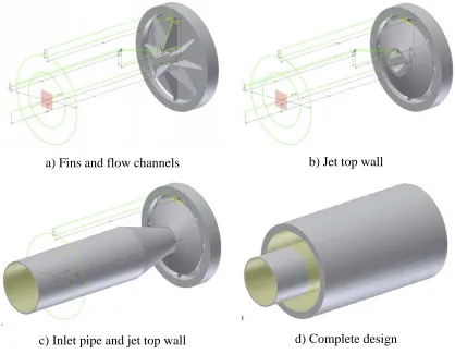
The first option investigated as a solution for thermal management of wide beam area x-ray sources has its roots in a study of smaller scale targets, [9], [10], and assumes an impinging cooling jet on the back of the target. Based on the recommendations from [9], [10], the target area of the original prototype design has been magnified by a factor of 4.04 and the rest of the dimensions adjusted accordingly, as presented in Table 3.1. Additionally, eight circumferential evenly distributed fins have been added to the back of the target which serves the following purposes:
Table 3.1 – Initial design 01 characteristics
Parameter Value Inlet diameter [mm / inch] 68.0 / 2.68
Inlet area [mm2 / inch2] 3631.68 / 5.63 Nozzle diameter [mm / inch] 28.8 / 1.13 Nozzle area [mm2 / inch2] 651.44 / 1.01 Outlet area [mm2 / inch2] 6625.65 / 10.27 Fin thickness [mm / inch] 2.0 / 0.0787 Heated target diameter [mm / inch] 132.4 / 5.213 Heated target area [mm2 / inch2] 13767.84 / 21.34 Target thickness [mm / inch] 10.8 / 0.425 Water volume [cm3 / inch3] 2457.5 / 149.97 Metal volume [cm3 / inch3] 1244.6 / 75.95
surroundings has been taken into account, the simulations provide conservative results. A summary of simulation results is presented in Table 3.2 and 3.3.
a) Fins and flow channels b) Jet top wall
c) Inlet pipe and jet top wall d) Complete design
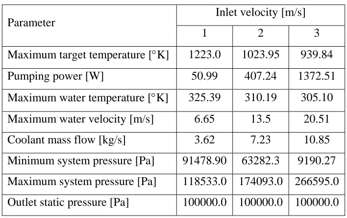
Table 3.2 – Initial design 01 simulation results (SI units)
Parameter Inlet velocity [m/s]
1 2 3 Maximum target temperature [°K] 1223.0 1023.95 939.84 Pumping power [W] 50.99 407.24 1372.51 Maximum water temperature [°K] 325.39 310.19 305.10 Maximum water velocity [m/s] 6.65 13.5 20.51 Coolant mass flow [kg/s] 3.62 7.23 10.85 Minimum system pressure [Pa] 91478.90 63282.3 9190.27 Maximum system pressure [Pa] 118533.0 174093.0 266595.0 Outlet static pressure [Pa] 100000.0 100000.0 100000.0
Table 3.3 – Initial design 01 simulation results (British units)
Parameter Inlet velocity [ft/s]
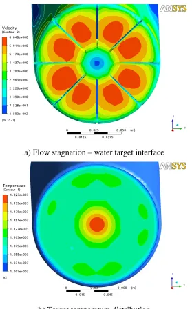
a) Flow stagnation – water target interface
b) Target temperature distribution
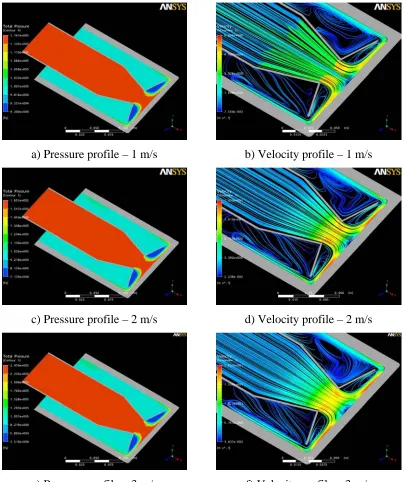
a) Pressure profile – 1 m/s b) Velocity profile – 1 m/s
c) Pressure profile – 2 m/s d) Velocity profile – 2 m/s
High mass flow rates result in increased maximum water velocity which may raise additional issues related to vibrations and possible material erosion and would require further investigation. Generally, the maximum pressure of the system becomes an important factor since it is desirable to have a high flow - low pressure cooling system.
Based on Figure 3.3, an evaluation of pressure and velocity profiles in the radial flow channels of this design is presented. Although maximum target temperatures are reduced with increasing inlet velocity, there are several shortcomings that need to be highlighted. For any inlet velocity, as the water exits the jet and hits the back of the target, a vortex region develops directly under the jet top wall, as seen in Figure 3.3 – b), d) and f). In this region, a pronounced drop in pressure is observed, as shown by Figure 3.3 – a), c) and e). As the inlet water velocity increases, the pressure drop becomes more and more significant. An increase in water temperature in this region may cause localized boiling to occur.
3.2.2 Initial Design 02
The presence of a flow stagnation point in the center of the target is one of the most significant drawbacks of initial design 01. In order to mitigate this issue, a new approach has been envisioned. The main attribute of this design is to change the flow direction from a direction that is perpendicular to the back of the target to one that is parallel to the back of the target. This idea is embodied in the initial design 02.
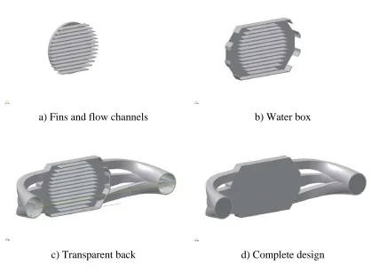
a) Fins and flow channels b) Water box
c) Transparent back d) Complete design
As illustrated in Figure 3.4, an array of flow channels is positioned horizontally on the back of the target. The water flows through these channels from right to left. The flow channels are enclosed in the water box. The water is supplied to the water box through three distribution channels which are connected to a common inlet header. The heated water is discharged from the water box through the three channels on the left which converge in a common outlet header. Because of the high velocity water jet that sweeps the back of the target, no obvious flow stagnation points are likely to develop.
Table 3.4 – Initial design 02 characteristics
Parameter Value Inlet diameter [mm / inch] 56.0 / 2.205
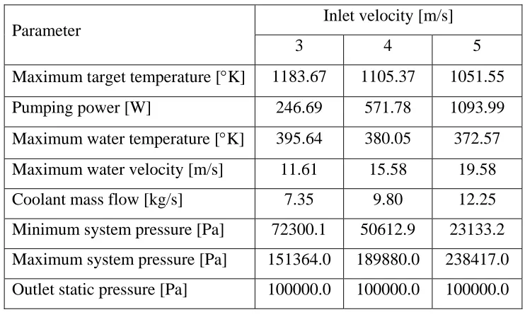
The heated area of the target is the same as for initial design 01 and the simulations were performed at the same power level of 180 kW. The inlet water temperature is 293 °K (67.73 °F) and inlet coolant velocities considered in the performance analysis of this design are 3, 4 and 5 m/s (9.84, 13.12 and 16.4 ft/s).
Table 3.5 – Initial design 02 simulation results (SI units)
Parameter Inlet velocity [m/s]
3 4 5 Maximum target temperature [°K] 1183.67 1105.37 1051.55 Pumping power [W] 246.69 571.78 1093.99 Maximum water temperature [°K] 395.64 380.05 372.57 Maximum water velocity [m/s] 11.61 15.58 19.58 Coolant mass flow [kg/s] 7.35 9.80 12.25 Minimum system pressure [Pa] 72300.1 50612.9 23133.2 Maximum system pressure [Pa] 151364.0 189880.0 238417.0 Outlet static pressure [Pa] 100000.0 100000.0 100000.0
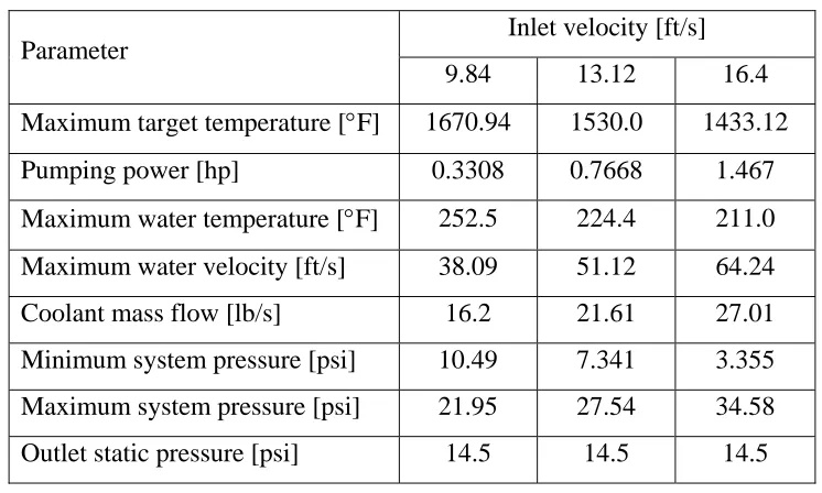
Table 3.6 – Initial design 02 simulation results (British units)
Parameter Inlet velocity [ft/s]
9.84 13.12 16.4 Maximum target temperature [°F] 1670.94 1530.0 1433.12 Pumping power [hp] 0.3308 0.7668 1.467 Maximum water temperature [°F] 252.5 224.4 211.0 Maximum water velocity [ft/s] 38.09 51.12 64.24 Coolant mass flow [lb/s] 16.2 21.61 27.01 Minimum system pressure [psi] 10.49 7.341 3.355 Maximum system pressure [psi] 21.95 27.54 34.58 Outlet static pressure [psi] 14.5 14.5 14.5
a) Velocity streamline b) Target temperature profile
c) Water temperature profile d) Pressure profile
e) Velocity vector profile f) Channels inlet-outlet pressure
A very interesting phenomenon has been identified during the post processing of simulation results. Not only do the low flow channels receive insufficient flow to ensure adequate target cooling, but the direction of the flow in these channels is opposite to the direction in the rest of the channels. Figure 3.5.e) presents the normalized velocity vector profile at the target mid-plane which provides a clear indication of flow reversal. Although this finding seemed to be surprising initially, the pressure distribution profile at the inlet (on the left) and exit (on the right) of the flow channels, Figure 3.5.f), provides additional information that supports this behavior.
While initial design 02 eliminated the flow stagnation point, unequal flow distribution raises concerns regarding adequate management of the target thermal load and maintaining forced convection as the heat transfer mechanism of choice. At the same time, high water inlet velocities require substantial pumping power while operating the cooling system at low pressure level is desirable. The idea of supplying relatively equal mass flow to each channel is explored further since designs with horizontal flow channels show good potential.
3.2.3 Initial Design 03
Circular inlet and outlets are selected to simplify coupling of this system to the pumping and heat removal systems. Also, the geometry of the inlet duct has been chosen such that the inlet area is greater than the total area of the flow channels such that coolant acceleration is achieved. Additionally, the curvature radius for the inlet and outlet ducts provides a smooth change in the flow direction which reduces the pressure losses associated with the fluid flow. The presence of fins, which also serve as flow channel walls, increases the heat transfer from the target to the coolant.
a) Target back b) Fins and flow channels
c) Water box d) Complete design
The target area subjected to a power input of 180 kW is the same as for initial design 01 and initial design 02. The material used in the simulations of target thermal response is copper and the coolant inlet temperature is 293°K (67.73°F). Simulations have been performed for inlet water velocities of 1, 2 and 3 m/s (3.28, 6.56 and 9.84 ft/s).
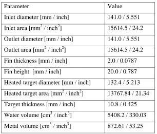
Table 3.7 – Initial design 03 characteristics
Parameter Value Inlet diameter [mm / inch] 141.0 / 5.551
Inlet area [mm2 / inch2] 15614.5 / 24.2 Outlet diameter [mm / inch] 141.0 / 5.551 Outlet area [mm2 / inch2] 15614.5 / 24.2 Fin thickness [mm / inch] 2.0 / 0.0787 Fin height [mm / inch] 20.0 / 0.787 Heated target diameter [mm / inch] 132.4 / 5.213 Heated target area [mm2 / inch2] 13767.84 / 21.34 Target thickness [mm / inch] 10.8 / 0.425 Water volume [cm3 / inch3] 5408.2 / 330.03 Metal volume [cm3 / inch3] 872.61 / 53.25
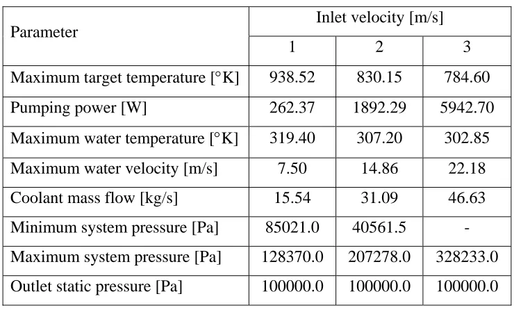
Table 3.8 – Initial design 03 simulation results (SI units)
Parameter Inlet velocity [m/s]
1 2 3 Maximum target temperature [°K] 938.52 830.15 784.60 Pumping power [W] 262.37 1892.29 5942.70 Maximum water temperature [°K] 319.40 307.20 302.85 Maximum water velocity [m/s] 7.50 14.86 22.18 Coolant mass flow [kg/s] 15.54 31.09 46.63 Minimum system pressure [Pa] 85021.0 40561.5 - Maximum system pressure [Pa] 128370.0 207278.0 328233.0 Outlet static pressure [Pa] 100000.0 100000.0 100000.0
Table 3.9 – Initial design 03 simulation results (British units)
Parameter Inlet velocity [ft/s]
The maximum water temperature is less than the boiling temperature over the entire fluid domain. One of the disadvantages of this design is the high pumping power required to maintain relatively large mass flows through the cooling channel. Additional issues, such as vibrations and erosion, may arise from high maximum water velocity on its path through the cooling channels.
The simulations revealed flow patterns which were not obvious when the initial design 03 geometry was originally conceived. As mentioned above, a high inlet area is beneficial because it allows a relatively small and equally distributed inlet velocity to be accelerated to values that ensure adequate target cooling. The outlet duct was constructed symmetrically to the vertical mid plane and, consequently, the outlet has the same area as the inlet.
Due to high velocity gained through acceleration, the curvature of the outlet duct and the high area of the outlet duct, the water velocity in the region starting from the flow channels exit to the outlet does not present a uniform distribution over the entire flow area. Also, the pressure distribution in this region is skewed such that a high pressure domain is located closer to the outward wall of the outlet flow duct and the low pressure domain establishes inwards.
solution accuracy, increases the computational effort and the uncertainty related to the flow conditions in the domain of interest.
Initial design 03 provided the opportunity to observe relevant phenomena for future design improvement. Two important remarks, which will guide the approach to the final design, need to be highlighted. First, a reduction in the outlet area would eliminate the formation of vortexes at the outlet with beneficial effects on the ANSYS CFX-Solver performance and overall solution convergence.
a) Velocity streamline b) Target temperature profile
c) Water temperature profile d) Pressure profile
e) Inlet-outlet pressure profile f) Velocity vector profile at outlet
3.3 Final Design
This chapter is dedicated to the detailed presentation of the final design adopted in this study as the most effective solution to complete thermal management of wide beam area x-ray sources. The final design incorporates the improvements drawn from the earlier designs and takes advantage of the CFD modeling experience and insight gained during these studies. The information presented in this section is structured in four parts. The first part deals with the geometry design description and material properties. The second part provides information about the mesh and meshing techniques employed. The CFD model construction details are unveiled in the third part. Finally, a roadmap that offers a clear and concise design performance evaluation is shown in the fourth part.
3.3.1 Geometry
The final design comes in three distinct versions which differ only in total target wall thickness. Figure 3.12 presents a sectional view and highlights of the three versions of the final design.
a) Final design transversal view
b) Final design ver.01
c) Final design ver.02
d) Final design ver.03
Table 3.10 – Final design features
Parameter Design version
01 02 03 Inlet diameter [mm / inch] 140.0 / 5.51 140.0 / 5.51 140.0 / 5.51
Inlet area [mm2 / inch2] 15393.8 / 23.9 15393.8 / 23.9 15393.8 / 23.9 Fin thickness [mm / inch] 2.0 / 0.0787 2.0 / 0.0787 2.0 / 0.0787 Fin height [mm / inch] 16.0 / 0.63 16.0 / 0.63 16.0 / 0.63 Fin length [mm / inch] 160.0 / 6.3 160.0 / 6.3 160.0 / 6.3 Fin spacing [mm / inch] 10.0 / 0.394 10.0 / 0.394 10.0 / 0.394 Water box wall thickness
[mm / inch] 1.0 / 0.0394 1.0 / 0.0394 1.0 / 0.0394 Cooling channel height
[mm / inch] 16.0 / 0.63 16.0 / 0.63 16.0 / 0.63 Cooling channel width
[mm / inch] 8.0 / 0.315 8.0 / 0.315 8.0 / 0.315 Heated target diameter
[mm / inch] 140.0 / 5.51 140.0 / 5.51 140.0 / 5.51 Heated target area [mm2 / inch2] 15393.8 / 23.9 15393.8 / 23.9 15393.8 / 23.9 Target wall thickness
[mm / inch] 0.2 / 0.00787 0.4 / 0.015 0.6 / 0.023 Total target thickness
The material used for the final target design is molybdenum. Since this material is not provided in the ANSYS materials database, it has to be defined by the analyst. The properties required by ANSYS are listed in Table 3.11, [11].
Table 3.11 – Molybdenum properties Thermodynamic state Solid
Property Value Molar mass [g/mol] 95.94
Density [g/cm3] 10.22
Specific heat capacity [kJ/kg·°K] 0.255 Thermal conductivity [W/m·°K] 138.0
3.3.2 Mesh
Tetra mesh employs several meshing techniques to fill the volume of interest with tetrahedral elements and generate a surface mesh on the object surface. The positions of edges and vertices in the mesh are determined based on the prescribed points and curves loaded from the geometry file. To improve mesh quality, Tetra incorporates a powerful smoothing algorithm, as well as capability to provide local adaptive mesh refinement and coarsening. The steps required to obtain a mesh are presented further. It should be emphasized that the accuracy of the CFD model and the rapid convergence of the CFD solution are strongly dependent on the successful generation of a quality mesh.
The geometry repair/clean up is the first step in generating a Tetra mesh. This ensures that the geometry is free of any flaws that would inhibit the mesh creation. To create a mesh, Tetra requires that the model is a closed volume. If there are any holes (gaps or missing surfaces) in the geometry larger than the local tetras, the meshing algorithm will be unable to close the volume and to complete the mesh creation. It is the responsibility of the analyst to fix the surface data and to eliminate these holes.
The second step requires that the geometry details be preserved while the mesh is created. In addition to a closed set of surfaces that encloses the volume of interest, Tetra requires curves and points where hard features, such as hard angles and corners, to be captured in the mesh. Thus, the mesh provides accurate representation of the initial geometry.
elements in regions of secondary importance, while in the areas of interest coarser mesh may not allow the investigated phenomena to be well represented and understood.
The Tetra mesh creation uses the Octree mesh method, [12] and [13], which is based on the spatial subdivision algorithm that ensures refinement of the mesh where necessary, but maintains larger elements where possible, allowing for faster computation. Once the “root” tetrahedron, which encloses the entire geometry, has been initialized, Tetra subdivides the root tetrahedron until all the element size requirements are met. The subdivision is performed such that elements sharing a face or an edge would not be different in size by more than a factor of 2. After the subdivision process is complete, Tetra makes the mesh conformal. This ensures that each pair of adjacent elements will share an entire face. At this point, the mesh does not respect the given geometry. Next, the mesher rounds the nodes of the mesh to the prescribed points, prescribed curves or model surfaces. Tetra cuts away all the mesh that can not reach a material point from the geometrical domain. Finally, the mesh is smoothed by moving nodes, merging nodes, swapping edged and, if required, by deleting bad elements.
Table 3.12 – Final design mesh characteristics
Part Final design
01 02 03
Inlet
Triangles 2272 2652 2622
Nodes 1137 1327 1312
Outlet
Triangles 610 678 676
Nodes 306 340 339
Heated target area
Triangles 8359 9543 10242
Nodes 4300 5261 5237
Molybdenum
Tetrahedrons 211343 210020 237427
Nodes 59076 58746 63647
Faces 99416 99066 100922
Water
Tetrahedrons 870122 863279 860338
Nodes 175237 173910 173392
Faces 113910 113392 113448
Total
Tetrahedrons 1081465 1073299 1097765
Nodes 234313 232656 237039
3.3.3 CFD Model
The development of each final design CFD model starts by defining a blank project and loading the appropriate mesh. Once ANSYS CFX-Pre finishes the mesh loading, the first step is to define the domains based on the geometry contained in the mesh. A domain usually consists of a closed geometrical volume which either can be solid, fluid or porous.
For the purpose of this research, two domains have been defined: one solid (molybdenum target) and one fluid (water). The preprocessor automatically creates an interface between the solid and the fluid domain in order to allow heat transfer to be calculated. The flow conditions at the limits of the fluid domain are specified through boundary conditions. For the water inlet, an Inlet boundary condition has been specified and for the water outlet an Outlet boundary is imposed.
To model the heat addition to the target, a Wall type boundary condition is employed for the heated target area. The heat flux on the heated target area can be specified either as a constant value or as a variable which stores spatial heat flux distribution. Details on the boundary conditions for the fluid and solid domain are available in Table 3.13.
Table 3.13 – Model boundary condition details Boundary
condition Details
Inlet Flow regime: Subsonic
Mass and momentum: Normal speed
Turbulence: Medium
Heat transfer: Temperature
Outlet Flow regime: Subsonic
Mass and momentum: Average static pressure
Pressure averaging: Average Over
Whole Outlet
-
Wall Heat transfer:
Heat flux in - - -
A solution to a CFD problem is obtained by resolving various equations using the appropriate boundary conditions and models. At any moment during the calculation, each equation will not be completely satisfied, and the “residual” of an equation provides a measure of the difference between the left-hand-side of the equation and the right-hand-side of the equation at any point in space. If the solution is exact, the residual is zero meaning that each relevant finite volume equation is satisfied precisely. This is not the case because the equations model the physics approximately.
The RMS residual is obtained by taking all the residuals throughout the domain, squaring them, taking the mean, and then taking the square root of the mean. For any simulation in this study, the maximum RMS residual is less than 1·10-5. These provisions are necessary to ensure reasonable numerical accuracy for the results presented herein.
ANSYS CFX-Solver has two classes of executables: default (single precision) and double precision. Double precision Solver executables store basic floating point numbers as 64 bit words. These executables permit more accurate numerical mathematical operations. Double precision accuracy might be needed if the computational domain involves a huge variation in grid dimensions, aspect ratio, pressure range, etc. The double precision Solver has been the standard choice for all simulations performed as part of this thesis.
3.3.4 Evaluation Roadmap
1. For each final design
2. For each inlet water velocity
Simula
tion 3.1 For a uniform heat flux
distribution, determine: a) Maximum target temperature
b) Pumping power c) Water subcooling margin
3.2 For a non-uniform heat flux distribution, determine heat flux maps that lead either to: a) Target melting temperature b) Water boiling
Post-proc
ess
ing
5.1 Create surface plots for: a) Normalized maximum target temperature b) Normalized pumping power
5.2 Create surface plot for normalized
maximum peak to average ratio
6.1 Develop equations for normalized surface plots from Step 5.1
6.2 Develop equation for normalized surface plot from Step 5.2
As previously mentioned, three versions of the final design have been investigated, each corresponding to a total target thickness of 1.2 mm (0.0472 inch), 1.4 mm (0.0551 inch) and 1.6 mm (0.063 inch). For each version, water inlet velocity has been varied from 0.6 m/s (1.97 ft/s) to 1.2 m/s (3.94 ft/s) in increments of 0.1 m/s (0.328 ft/s). As mentioned in Figure 3.13, Step 3.1 and 3.2, uniform heat flux and non-uniform heat flux distributions have been imposed as boundary conditions on the heated target area for each combination of wall thickness and water inlet velocity. For simulations performed at Step 3.1, the uniform heat flux is determined based on a maximum target power of 180 kW and a target area of 15393.8 mm2 (23.9 inch2) which yields 11.693·106 W/m2 (3.707·106 Btu/h·ft2).
Non-uniform heat flux distributions arise from the practical difficulty of generating a uniform electron beam. There are two parameters that identify a non-uniform distribution. The first one is the average heat flux of the distribution, which for the purpose of this study is maintained at the same value as the uniform distribution value. The second parameter is the peak to average ratio which is obtained by dividing the highest heat flux value by the average heat flux value for a distribution. The method for constructing a non-uniform distribution is presented further.
representations of the normal distribution is provided by the continuous probability density function (PDF), as seen in Figure 3.14.
0.0 0.2 0.4 0.6 0.8 1.0 1.2 1.4 1.6 1.8 2.0
-1.0 -0.8 -0.6 -0.4 -0.2 0.0 0.2 0.4 0.6 0.8 1.0
Figure 3.14 – Continuous probability density function for normal distribution
The continuous probability density function is given by:
(
)
( 2)2 2 x e 2 1 , , x f σ μ − − π σ = σ μ (3.1)
the most limiting position for the maximum heat flux value, the expected value of the PDF is set to zero for all distributions herein.
The non-uniform heat flux distribution required as input in ANSYS-CFX has to be provided in the format: X coordinate, Y coordinate, Z coordinate and heat flux value. Because the flux distribution is on a planar surface perpendicular on X-Axis, the X coordinate is constant. Consequently, the problem reduces to generating an n × n matrix of heat flux values – M(i,j), i=1..n, row index, j=1..n, column index, n=21 – which satisfies the following requirements:
- the average value of the elements in the matrix is constant, - the elements in any row or column follows a normal distribution,
- the matrix has quadrant symmetry, the elements positioned at equal distance left-right from the center column and up-down from the center row have the same value.
- different ratios of the maximum value to the average value have to be obtained by changing a single parameter.
( )
(
(
)
)
,k 1..10 k , 11 M 11 , 11 M 1 , kF = = (3.2)
Next, the remaining 20 rows of elements in matrix M have to be calculated. The values for elements in a row are determined by dividing the values from row 11 to the corresponding multiplication factor. For example, M(5,1..21) values are calculated using:
( )
( )
( )
,j 1..21 1 , 5 F j , 11 M j , 5M = = (3.3)
After all the above operations, the elements from matrix M still have the values calculated using the probability density function. By multiplying all the elements by the uniform, average heat flux value, a complete non-uniform heat flux distribution is obtained. From this distribution, a peak to average ratio can be easily determined. There is one parameter of the probability density function which controls the shape and peak to average ratio for any heat flux distribution. This parameter is the standard deviation. A non-uniform heat flux distribution with desired peak to average ratio is obtained through fine tuning the standard deviation value.
beneficial because the heat flux values for the discarded points are very small. Selected heat flux distribution profiles can be seen in Appendix A.
Simulations performed using a uniform heat flux distribution, Figure 3.13 - Step 3.1, provide as output the maximum target temperature, the required pumping power and the water subcooling margin for each case analyzed. The subcooling margin has been calculated as the difference between water saturation temperature corresponding to the minimum total pressure and the maximum water temperature, within the whole fluid domain, obtained from simulation.
For simulations involving non-uniform heat flux distributions, Figure 3.13 - Step 3.2, the purpose was to determine the heat flux shape, uniquely identified by its peak to average ratio, which would produce a maximum target temperature equal to the target melt temperature or would create favorable conditions for localized water boiling (subcooling margin equals to zero). For each target wall thickness and each water inlet velocity, the process is iterative and requires a large number of CFD runs.
obtained in which all variables values are between 0 and 1 and their dependence on total target thickness and water inlet velocity is preserved. Based on the normalized tables, surface plots are created to provide a visual representation of the data.
Chapter 4 Results
This chapter presents the CFD simulation results of the final design and consists of four parts. The first part will elaborate on the findings resulting from simulations considering the uniform heat flux distribution. The second part will examine the final design response for the case of a non-uniform heat. The construction of design solution space is detailed in the third part. Finally, result analysis is provided in the fourth part.
4.1 Uniform Heat Flux Distribution
As previously mentioned, a uniform heat flux distribution has been considered as part of final target design evaluation. The heat flux value imposed as boundary conditions is 11.693·106 W/m2 (3.707·106 Btu/h·ft2). The water inlet temperature for all simulations is 293°K (67.73 °F). The target material is molybdenum with a melting temperature of 2890°K (4742.33°F). The pressure drop across the target is determined as the difference between the average inlet pressure and the average outlet pressure. The pumping power associated with the coolant flow is calculated using Eq. (4.1) based on total mass flow, water density and the pressure drop. The average water density used in the Eq. (4.1) is 997 kg/m3 (62.24 lb/ft3).
p m
P Δ
ρ
Table 4.1 – Final design ver.01 simulation results (SI units)
Location / Parameter Water inlet velocity [m/s]
0.6 0.7 0.8 0.9 1.0 1.1 1.2 Inlet
Average pressure [Pa] 112206.0 116304.0 120973.0 126211.0 132018.0 138392.0 145.332.0
Average temperature [°K] 293.15 293.15 293.15 293.15 293.15 293.15 293.15
Outlet
Average velocity [m/s] 2.4 2.8 3.2 3.6 4.0 4.41 4.81
Average pressure [Pa] 102947.0 104012.0 105241.0 106634.0 108192.0 109913.0 111799.0
Average temperature [°K] 297.49 296.87 296.41 296.05 295.76 295.52 295.33
Maximum target temperature [°K] 801.41 754.94 718.31 688.61 664.01 643.27 625.54
Water domain
Minimum velocity [m/s] 0.55 0.65 0.75 0.84 0.93 1.03 1.12
Minimum pressure [Pa] 98948.1 98578.3 98155.6 97680.3 97152.3 96571.8 95938.5
Table 4.1 (continued)
Location / Parameter Water inlet velocity [m/s]
0.6 0.7 0.8 0.9 1.0 1.1 1.2 Water domain
Maximum velocity [m/s] 5.58 6.5 7.42 8.33 9.25 10.17 11.08
Maximum pressure [Pa] 114051.0 118821.0 124268.0 130389.0 137183.0 144649.0 152787.0
Maximum temperature [°K] 331.38 326.22 322.3 319.22 316.73 314.68 312.96
Mass flow rate [kg/s] 9.2 10.7355 12.2692 13.8028 15.3365 16.8701 18.4038
Pressure drop [Pa] 9259.0 12292.0 15732.0 19577.0 23826.0 28479.0 33533.0
Pumping power [W] 85.44 132.36 193.6 271.03 366.51 481.89 618.99
Table 4.2 – Final design ver.01 simulation results (British units)
Location / Parameter Water inlet velocity [ft/s]
1.97 2.3 2.62 2.95 3.28 3.61 3.94 Inlet
Average pressure [psi] 16.3 16.9 17.5 18.3 19.1 20.1 21.1
Average temperature [°F] 68 68 68 68 68 68 68
Outlet
Average velocity [ft/s] 7.87 9.19 10.5 11.8 13.1 14.5 15.8
Average pressure [psi] 14.9 15.1 15.3 15.5 15.7 15.9 16.2
Average temperature [°F] 75.8 74.7 73.9 73.2 72.7 72.3 71.9
Maximum target temperature [°F] 982.88 899.24 833.29 779.83 735.54 698.22 666.31
Water domain
Minimum velocity [ft/s] 1.8 2.13 2.46 2.76 3.05 3.38 3.67
Minimum pressure [psi] 14.4 14.3 14.2 14.2 14.1 14.0 13.9
Table 4.2 (continued)
Location / Parameter Water inlet velocity [ft/s]
1.97 2.3 2.62 2.95 3.28 3.61 3.94 Water domain
Maximum velocity [ft/s] 18.3 21.3 24.3 27.3 30.3 33.4 36.4
Maximum pressure [psi] 16.5 17.2 18 18.9 19.9 21 22.2
Maximum temperature [°F] 136.81 127.53 120.47 114.93 110.44 106.75 103.66
Mass flow rate [lb/s] 20.28 23.67 27.05 30.43 33.81 37.19 40.57
Pressure drop [psi] 1.35 1.79 2.29 2.84 3.46 4.13 4.87
Pumping power [hp] 0.1146 0.1775 0.2596 0.3635 0.4915 0.6462 0.8301
Table 4.3 – Final design ver.02 simulation results (SI units)
Location / Parameter Water inlet velocity [m/s]
0.6 0.7 0.8 0.9 1.0 1.1 1.2 Inlet
Average pressure [Pa] 112230.0 116336.0 121015.0 126264.0 132083.0 138470.0 145423.0
Average temperature [°K] 293.15 293.15 293.15 293.15 293.15 293.15 293.15
Outlet
Average velocity [m/s] 2.43 2.84 3.24 3.65 4.06 4.46 4.87
Average pressure [Pa] 103036.0 104131.0 105394.0 106824.0 108423.0 110190.0 112125.0
Average temperature [°K] 297.5 296.88 296.42 296.06 295.77 295.53 295.34
Maximum target temperature [°K] 817.313 771.1 734.676 705.15 680.687 660.111 642.506
Water domain
Minimum velocity [m/s] 0.56 0.65 0.75 0.84 0.93 1.03 1.12
Minimum pressure [Pa] 98548.2 98038.3 97455.9 96801.0 96073.7 95273.9 94401.4
Table 4.3 (continued)
Location / Parameter Water inlet velocity [m/s]
0.6 0.7 0.8 0.9 1.0 1.1 1.2 Water domain
Maximum velocity [m/s] 5.6 6.52 7.44 8.36 9.28 10.19 11.11
Maximum pressure [Pa] 114385.0 119262.0 124824.0 131082.0 138023.0 145649.0 153957.0
Maximum temperature [°K] 330.76 325.67 321.81 318.77 316.33 314.31 312.62
Mass flow rate [kg/s] 9.2021 10.7358 12.2695 13.8032 15.3369 16.8706 18.4043
Pressure drop [Pa] 9194.0 12205.0 15621.0 19440.0 23660.0 28280.0 33298.0
Pumping power [W] 84.86 131.42 192.24 269.14 363.96 478.54 614.67
Table 4.4 – Final design ver.02 simulation results (British units)
Location / Parameter Water inlet velocity [ft/s]
1.97 2.3 2.62 2.95 3.28 3.61 3.94 Inlet
Average pressure [psi] 16.3 16.9 17.6 18.3 19.2 20.1 21.1
Average temperature [°F] 68 68 68 68 68 68 68
Outlet
Average velocity [ft/s] 7.97 9.32 10.6 12.0 13.3 14.6 16.0
Average pressure [psi] 14.94 15.1 15.29 15.49 15.73 15.98 16.26
Average temperature [°F] 75.83 74.71 73.89 73.24 72.72 72.28 71.94
Maximum target temperature [°F] 1011.5 928.31 862.75 809.6 765.57 728.53 696.84
Water domain
Minimum velocity [ft/s] 1.84 2.13 2.46 2.76 3.05 3.38 3.67
Minimum pressure [psi] 14.29 14.22 14.13 14.04 13.93 13.82 13.69
Table 4.4 (continued)
Location / Parameter Water inlet velocity [ft/s]
1.97 2.3 2.62 2.95 3.28 3.61 3.94 Water domain
Maximum velocity [ft/s] 18.37 21.39 24.41 27.43 30.45 33.43 36.45
Maximum pressure [psi] 16.59 17.3 18.1 19.01 20.02 21.12 22.33
Maximum temperature [°F] 135.7 126.5 119.6 114.1 109.7 106.1 103.0
Mass flow rate [lb/s] 20.29 23.67 27.05 30.43 33.81 37.19 40.57
Pressure drop [psi] 1.34 1.77 2.27 2.82 3.44 4.11 4.83
Pumping power [hp] 0.1138 0.1762 0.2578 0.3609 0.4881 0.6417 0.8243
Table 4.5 – Final design ver.03 simulation results (SI units)
Location / Parameter Water inlet velocity [m/s]
0.6 0.7 0.8 0.9 1.0 1.1 1.2 Inlet
Average pressure [Pa] 112224.0 116329.0 121006.0 126253.0 132070.0 138455.0 145408.0
Average temperature [°K] 293.15 293.15 293.15 293.15 293.15 293.15 293.15
Outlet
Average velocity [m/s] 2.43 2.84 3.25 3.65 4.06 4.47 4.87
Average pressure [Pa] 103039.0 104135.0 105399.0 106381.0 108431.0 110200.0 112137.0
Average temperature [°K] 297.52 296.9 296.43 296.07 295.78 295.54 295.35
Maximum target temperature [°K] 829.222 784.001 748.303 719.331 695.304 675.029 657.676
Water domain
Minimum velocity [m/s] 0.56 0.65 0.74 0.84 0.93 1.02 1.12
Minimum pressure [Pa] 98714.7 98263.9 97749.5 97171.3 96529.2 95823.2 95053.4
Table 4.5 (continued)
Location / Parameter Water inlet velocity [m/s]
0.6 0.7 0.8 0.9 1.0 1.1 1.2 Water domain
Maximum velocity [m/s] 5.57 6.49 7.41 8.32 9.24 10.15 11.07
Maximum pressure [Pa] 114248.0 119132.0 124666.0 130886.0 137789.0 145376.0 153644.0
Maximum temperature [°K] 333.12 327.73 323.63 318.77 317.82 315.68 313.89
Mass flow rate [kg/s] 9.2021 10.7358 12.2695 13.8032 15.3369 16.8706 18.4043
Pressure drop [Pa] 9185.0 12194.0 15607.0 19422.0 23639.0 28255.0 33271.0
Pumping power [W] 84.78 131.31 192.07 268.89 363.64 478.11 614.17
Table 4.6 – Final design ver.03 simulation results (British units)
Location / Parameter Water inlet velocity [ft/s]
1.97 2.3 2.62 2.95 3.28 3.61 3.94 Inlet
Average pressure [psi] 16.28 16.87 17.55 18.31 19.16 20.08 21.09
Average temperature [°F] 68 68 68 68 68 68 68
Outlet
Average velocity [ft/s] 7.97 9.32 10.66 11.98 13.32 14.67 15.98
Average pressure [psi] 14.94 15.1 15.29 15.43 15.73 15.98 16.26
Average temperature [°F] 75.87 74.75 73.9 73.26 72.73 72.3 71.96
Maximum target temperature [°F] 1032.9 951.53 887.28 835.13 791.88 755.38 724.15
Water domain
Minimum velocity [ft/s] 1.84 2.13 2.43 2.76 3.05 3.35 3.67
Minimum pressure [psi] 14.32 14.25 14.18 14.09 14.0 13.9 13.79
Table 4.6 (continued)
Location / Parameter Water inlet velocity [ft/s]
1.97 2.3 2.62 2.95 3.28 3.61 3.94 Water domain
Maximum velocity [ft/s] 18.27 21.29 24.31 27.3 30.31 33.3 36.32
Maximum pressure [psi] 16.57 17.28 18.08 18.98 19.98 21.09 22.28
Maximum temperature [°F] 139.95 130.24 122.86 114.12 112.41 108.55 105.33
Mass flow rate [lb/s] 20.29 23.67 27.05 30.43 33.81 37.19 40.57
Pressure drop [psi] 1.34 1.77 2.27 2.82 3.43 4.1 4.83
Pumping power [hp] 0.1137 0.1761 0.2576 0.3606 0.4876 0.6412 0.8236
Data mining the results presented in Table 4.1 – 4.6, maximum target temperature as function of total target thickness and inlet water temperature is obtained. Similarly, pumping power is correlated with the total target thickness and inlet water temperature. Synthetic data for both dependences are shown in Table 4.7 and 4.8.
Table 4.7 – Maximum target temperature dependence, °K
Water inlet velocity [m/s]
Total target thickness [mm]
1.2 1.4 1.6
0.6 801.415 817.313 829.222
0.7 754.948 771.1 784.001
0.8 718.31 734.676 748.303
0.9 688.61 705.15 719.331
1.0 664.007 680.687 695.304
1.1 643.271 660.111 675.029
Table 4.8 – Pumping power dependence, W
Water inlet velocity [m/s]
Total target thickness [mm]
1.2 1.4 1.6
0.6 85.44 84.86 84.78
0.7 132.36 131.42 131.31
0.8 193.60 192.24 192.07
0.9 271.03 269.14 268.89
1.0 366.51 363.96 363.64
1.1 481.89 478.54 478.11
1.2 618.99 614.67 614.17