New Approach of Performance Analysis of RLS Adaptive Filter Using a Block-wise Processing

New Approach of Performance Analysis of RLS

Adaptive Filter Using a Block-wise Processing

HAMZÉ HAIDAR ALAEDDINE

HKS Laboratory, Electronics and Physics Dept. Faculty of Sciences I, Lebanese University, Lebanon

ALAA A. GHAITH

HKS Laboratory, Electronics and Physics Dept. Faculty of Sciences I, Lebanese University, Lebanon

MOSTAFA AL-SAHILI

HKS Laboratory, Electronics and Physics Dept. Faculty of Sciences I, Lebanese University, Lebanon

MOUENES FADLALLAH

HKS Laboratory, Electronics and Physics Dept. Faculty of Sciences I, Lebanese University, Lebanon

Abstract:

This paper presents an efficient implementation of adaptive filtering for echo cancelers for teleconference systems during single-talk situation. The problem of echo cancellation is recurrent for all modern communication systems. The general solution consists to estimate the room impulse response and reproduce the echo signal in order to subtract it from the received signal and then reduce its effect at the far-end user side and consequently improves the conversation quality. Several types of adaptive algorithms exist in the estimation process. The most popular echo canceler (EC) uses Least Mean Squares (LMS) or Recursive Least Squares (RLS) adaptive filter. In practice, the choice of an algorithm must be made bearing in mind some fundamental aspects:

- Reduced computational complexity algorithms.

The literature shows that the RLS algorithm is more efficient than the LMS algorithm. It allows to reach an echo reduction of 46 dB which is large enough than the required threshold. Moreover, it presents a faster convergence compared to the LMS algorithm during single-talk situation. However, the implementation of the RLS algorithm applied to acoustic echo cancellation system has shown the disadvantage of requiring a strong computational complexity. To reduce the computational cost of this algorithm, we propose a new version of the RLS algorithm based on the Fast Fourier Transform (FFT) and on the recursive operation over a block of N samples instead of one sample.

Simulation results show that the proposed algorithm has a faster adaptation convergence, during single-talk situation, and reduce considerably the hardware resources needed for the implementation and the execution time in terms of N.

Key words: Acoustic Echo Cancellation, Adaptive Filter, Adaptive algorithm, LMS Algorithm, RLS Algorithm.

1. INTRODUCTION

implemented in order to preserve the quality of the communication.

Adaptive filtering is proved to be an effective tool for this task for several years: In fact, filtering is made adaptive if its parameters are modified according to a given criterion, as soon as a new value of the signal becomes available. Adaptation of the adaptive filter coefficients has been carried out for decades using the LMS (Least Mean Squares) algorithms and has also been performed with recursive type methods such as RLS (Recursive Least Squares).

The RLS algorithm makes it possible to obtain efficient results when identifying the acoustic channel, that is to say with a faster convergence rate compared to the LMS algorithm. On the other hand, its implementation is more complex and costly.

The choice of the optimization algorithm will be made according to two criteria, which are; The speed of convergence which will be the number of iterations necessary to converge close enough to the optimal solution and the computational complexity of the adaptive algorithm.

The main objective of this paper is to propose a new version of the adaptive filtering algorithm RLS by processing it in blocks of samples. This block processing method has the following advantages:

 It processes a block of samples at each iteration, which reduces the calculation execution time.

 It involves a series of convolution products which can be realized by the implementation of the fast Fourier transform.

 It allows an implementation on a fixed-point processor.

 Its convergence rate is fairly rapid.

recalls the theory of adaptive filtering. It also recalls and compares the two different adaptation algorithms, LMS and RLS. Section 3 describes the method of processing the RLS algorithm by sample blocks and highlights the value of using this method in signal processing. It also presents an implementation using the FFT of this new algorithm. In the last section, numerical results of the realization of the RLS algorithm by blocks using the FFT are given.

2. ACOUSTIC ECHO

The acoustic echo is caused by the transmission of the signal emitted by the loudspeaker and received by the microphone: this transmission is composed of a direct path and multiple reflections captured by the microphone, and consequently return to the speaker who spoke, in a distant room, his own signal.

The impulse response of the echo path is in the form of a direct wave and a succession of waves reflected from the walls of a particular room. The long duration of the echo path is mainly due to the low speed of sound in the air. When the acoustic echo is present in an inconvenient way, it is necessary to remove it [Gilloire 1987].

2.1. Acoustic echo cancellation

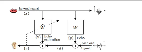
Figure 1. Principle of the acoustic echo cancellation system

The echo cancellation is performed by identifying the impulse response of the echo path by adaptive filtering represented by its coefficients, wˆ_k 



wˆ

_{   }

0 wˆ1wˆ

_

L1

_



T, where k represents the discrete time. Typically, the echo cancellation system uses two main adaptive algorithms which are: LMS (Least Mean Squares) and Recursive Least Squares (RLS).

2.2. Acoustic echo cancellation algorithms

2.2.1. Least Mean Square Algorithm (LMS)

The Least Mean Square algorithm (LMS) designed in 1959, is based on the gradient method which computes and updates recursively the weights. This gradient method consists of obtaining from a given vector wˆk, a vector wˆk1by incrementing of the vector wˆkin the opposite direction of the gradient of the

cost function



: [Kazuo 1990], [George 1999], [Paleologu 2010]:







  1 ˆ 1₂

ˆ_k w_k

w ₍₁₎

where



is the adaptation step of the gradient algorithm which controls the convergence of the adaptive filter.

The cost function



, which will minimize the mean squared error (MSE), is defined by:

 

2

k k Ee

The error ek is a quadratic form of the weights, and intuitively,

the optimal solution is obtained by stepwise correcting the weighting vector in the direction of the minimum.

k T k k k k

k

d

y

d

x

w

e





ˆ





ˆ

₍₃₎

- xk [Xk Xk1 XkL1]T _{is the input sequence.}

- yˆk is the echo estimation that can be obtained by filtering the

input sequence xk with the coefficients wˆk of the filter as

follow:

 

k

T k n k L

n k

k

w

n

x

w

y

ˆ

ˆ

X

ˆ

1 0







 _

 ₍₄₎

Adaptation of the coefficients of the adaptive filter

w

ˆ

_according

to the LMS algorithm is given by:

k k k

k w x e

wˆ _1 ˆ 



₍₅₎

The computational complexity of the LMS algorithm is known: each iteration consists (2L + 1) multiplications and (2L) additions. It can be seen that the LMS algorithm has an extremely low computational complexity. On the other hand, for non-stationary signals, it is difficult to follow the variations of the input signal by adapting the coefficients of the adaptive filter by this algorithm, which gives a slow convergence. To solve this problem, we use the RLS algorithm.

2.2.2. Recursive Least Squares Algorithm (RLS)

To compensate the problem of the non-stationarity of the signal, we use the Recursive Least Squares (RLS) algorithm. In this method, instead of minimizing a statistical criterion established







   k

n n n k

d

y

0

2

ˆ



(6)

The signal estimation

 

d using the least-squares method and

an impulse response wˆk, is obtained when the cost function



k

is minimized.

By analogy with the LMS algorithm, the estimated impulse response of the RLS filter is therefore to be modified with each new iteration. To limit the number of computations, we use a recursive equation given by:

k k k

k w G e

wˆ _1 ˆ  ₍₇₎

k T k k k k

k

d

y

d

x

w

e





ˆ





ˆ

₍₈₎

The column vector G_k,_{with size L, is called the Kalman gain,} which can be defined as follows:

k k T k k k k

x

P

x

x

P

G

1 1 1 1

1

 _

  







(9) -



is a weighting factor that always takes a positive value: 0<<



_{≤1. This factor is also called forgetting factor because it is}

used to forget data that corresponds to a distant past.

- Pk is the inverse auto-correlation matrix of size (L×L), which

can be calculated recursively as follows:

              

 1 _{k 1}



_k T_{k k 1}

k

P

G

x

P

P



(10)





1 ,

0

.

I

L

P



 _{is a positive constant}

L

I _{is an identity matrix of size (L×L)}

The details of the calculations necessary to arrive at the formulation of the RLS algorithm which is represented by equations (8), (9) and (10) is given in the Appendix.

The computational complexity of the RLS algorithm is

multiplications/divisions implemented for the RLS algorithm at

each iteration is respectively of the order

2

L

2



1

,

and3L27L.

Then the RLS algorithm requires many more operations than the LMS algorithm.

2.3. Performance comparison of LMS and RLS algorithms

Numerical simulations were made in the single talk situation to evaluate the performance of the two adaptive algorithms LMS and RLS using MatLab programming software.

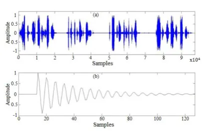
The two algorithms are evaluated by a speech signal and an echo path impulse response respectively presented in the two figures (2-a) and (2-b). In our study, we are interested in the case of a simple speech (presence of a distant signal only).

The problem that arises is that of choosing an optimization algorithm. This choice will be determined by the convergence speed of the filter and the computational complexity. The optimal algorithm is one that satisfies these two criteria.

The attenuation of the echo can be measured by the evolution of the convergence Nm of the adapted filter given by

the two algorithms LMS and RLS. The measurement is carried out in a conventional manner using the L successive samples, that is to say, at the index time

k

:















 



2 2 10

ˆ

10

w

w

w

log

N

_m

(11)

Where w _and

w

ˆ

_{denote respectively the impulse response and}

the estimated impulse response of the echo path.

the adaptation step



0.05, the forgetting factor





1

_and

.

8





Figure 2. (a) Input Signal (b) The impulse response of the echo path

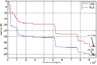
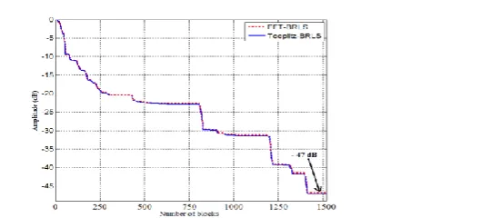
An echo cancellation system must provide echo attenuation of the order of 24 dB. The same system must be able to provide 40 dB echo attenuation for delays exceeding 25 ms. [Gilloire 1994] Figure (3) shows the evolution of the convergence of two adaptive algorithms, LMS and RLS as a function of the number of samples. This figure shows that the RLS (discontinuous line curve) algorithm has a faster convergence rate (-46 dB) than the LMS algorithm (-38.7 dB). The difference between the two convergence speeds can reach 7 dB.

The choice of the value of the coefficients is only an example to demonstrate the performance of the RLS algorithm with respect to the LMS algorithm. Any other choice of the coefficients can only show that the RLS algorithm remains the most efficient in terms of making the residual echo less audible at the output of the acoustic echo cancellation system.

systems, successively adapted by the LMS and the RLS. The echo cancellation system works well in the case of simple speech. We observed that the residual echo provided by the RLS algorithm becomes less audible compared to that provided by the LMS algorithm. On the other hand, the implementation of the RLS algorithm presented a significant global computational load compared to the LMS algorithm. Therefore, problems of execution time and complexity of computation always arise when we try to implement this algorithm in a real time processor. For these reasons, it is then necessary to reduce the costs of these operations to be processed. To remedy to this problem, a new technique to treat the RLS algorithm has been proposed in this article. This technique consists of processing the RLS algorithm by blocks of samples instead of processing it sample by sample.

Figure 3. Convergence of filter coefficients by the two algorithms

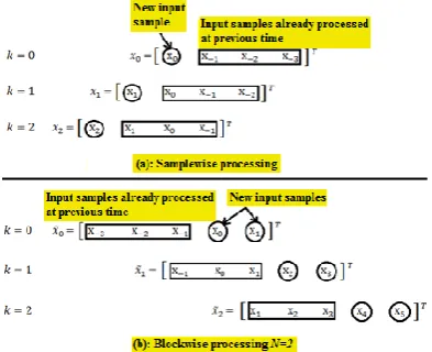
3. Recursive Least Square by Block Structure

block. This implies a reduction of the execution time and a reduction of the calculation complexity by a factor N, at least for the adaptation part.

In this section, we describe the block adaptive filtering procedure. The mathematical formulation of this procedure is obtained in vector form by processing the N samples of the

interval



kN;kNN1



at each iteration,

k

_{denoting the index}

of the block (

k

_∈ℕ).

Let wˆk the adaptive filter of length L designed to

estimate the acoustic feedback path and updated at each iteration

k

.

_{The estimated echo using a block-processed}

algorithm is given by: [Clark 1981], [Alaeddine 2012]:

      k k L k k k L N kN L kN L kN N kN kN kN N kN kN kN

k

R

w

w

w

w

y

~

.

ˆ

ˆ

ˆ

ˆ

~

1 1 0 X 2 X 1 X 2 X X 1 X 1 X 1 X X

























































            





















y

ˆ

kN

y

ˆ

kN1



y

ˆ

kNN1



T (12)

Where

R

k

~

is the Toeplitz matrix of size (N× L).

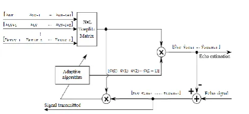
The principle of block processing is described by the figure (4). This figure shows that the mathematical formulation of the procedure for processing the RLS algorithm by blocks is

obtained by replacing the input vector

T L k k k k

x [X X _1 X _{ 1}] by the Toeplitz matrix in the adaptive equations of the filter. This algorithm will be called Toeplitz-BRLS.

The error vector (residual echo) of length N is given by:





T

N kN kN

kN

k  e e 1e  1



₍₁₃₎

where dk



dkN dkN 1 dkN N 1



T

~

  

Figure 4. Adaptive filtering by block structure

From the equations (12 and 13), it can be seen that block processing allows us to calculate N elements at each iteration

,

k _{unlike sample processing.}

The implementation of the Toeplitz-BRLS algorithm which is based on matrix computation is very complicated from a computational point of view. To remedy this problem, we propose to perform this calculation by the circular discrete convolution which can be made less expensive and does not modify the treatment to be carried out. The elements of the estimated echo signal, ~yk, will be calculated so that the

property of the circular convolution can be used as follows: [Khong 2005]

  _k

 

_k m

L

i kN m i i

k m

kN

w

w m

y

ˆ

1

ˆ

x

ˆ

x

0











  



(14)

where  represents the circular convolution and 0mN1. Similarly, the matrix product,

R

~

_kT



_k, _{in both equations (7) and}

(9) of the adaptive filter coefficient update can be calculated by the discrete convolution as follows:

k N

kN kN j j j k

T

k

e

x

R





 





  1

.

~

(15)

,

~

k T k k

R







_{corresponds to a cross-correlation whose coefficients}

ik

1

0

,

x

.

1 0









    

N

e

i

L

m kN m kN m i k



(16) If we put nkNm, the



ikcan be written in the form of a

convolution in the following way:

i n N

kN kN n n n i

ik

e

x

e

x

    





* 1

.



(17) From the equations (14) and (17), it can be seen that the

adaptive filtering by the proposed algorithm "Block-RLS (BRLS)" consists in calculating the circular convolution between the vectors wˆkand ~xk,of respective length N and

N+L-1, and the vectors



k and ~xk, where ~xk being the sequence of

the input signal defined by:

T N kN L kN L N k k

x [X ₁ X ₂ X ₁]

~      

  ₍₁₈₎ We can conclude that with our proposition, replacing the matrix

calculation, by the convolution product, the computational

complexity will be proportional to L instead of L2.

The adaptation of the coefficients of the adaptive filter by the proposed BRLS algorithm can be represented according to the equation:



k k



k k T k k k k

x

x

p

x

p

w

w







*

~

.

~

~

1

ˆ

ˆ

1 1 1 1 1      







(19) Following our proposal, the estimated echo is given by:

k k

k w x

y ˆ *~

~ _

(20)

Figure (5) shows the advantage of using the block processing method to reduce the execution time and in a particular case where the length of the block is equal to N = 2.

This figure demonstrates the interest of our proposal at the execution time: Indeed, if the length of the block is equal to

5.a), which processes only 3 new samples for the same number of iterations. So we can see that our proposal to process the RLS algorithm by blocks of samples allows us to reduce the execution time as a function of the length N of the block.

Figure 5. Representation of the input sequence by the two adaptation methods

A circular convolution in the time domain is equivalent to a term-to-term multiplication in the domain of the Fast Fourier Transform (FFT), which makes it possible to reduce the computational complexity and the execution time in the algorithms using the FFT.

3.1. Block-RLS by the Fast Fourier Transform

(FFT-BRLS)

The circular convolution presented in the BRLS algorithm can be calculated in the FFT domain with reduced computational complexity.

convolution between vectors wˆkand ~xk, and vectors



k and .

~ k

x_

Note that

Y

k

~

is the product of the circular convolution between

k

x

~

andwˆk:

 













M N L 





T

T k L M T k

k w x

Y~  ˆ 0_{1 }  ~ 0_{1   1}

(21)

 













 









T

L N M T k L M T

k FFT x

w FFT

FFT1 ˆ 0_{1 }  ~ 0_{1   1}



Where FFT and _FFT1 _{denote respectively the direct and}

inverse Fourier transforms. 0ij _{is a null matrix of size}

 

i j. For the calculation of the FFT, it is necessary to choose M power of 2. In general, we choose

M



N



L



1

_{(in our case}

L

N



_{) if this value is a power of 2, if not it is necessary to}

complete the vectors by a necessary samples of zero coefficients in order to give them a size equal to a power of 2, as shown in equation (21).

At each iteration k, the adaptation of the adaptive filter is then performed by calculating the circular convolution in the domain of the FFT _{following this expression:}







 









 







T L N M T k N M T k k

k w x

w

1 1

1

1 ˆ . 0 ~ 0

ˆ       

  



 ₍₂₂₎

 













 























_







_{  }T _{M NL} T

k L

M T

k

k

FFT

FFT

FFT

x

w

ˆ



.

1



0

₁

~

0

_{1 1}

Where

_~

_~

,

1

1 ₁

1 1 k k T k k

x

p

x

p

   











and . ]

[X ₁ X ₂ X ₁

~ T L kN N kN N N k k



_{is a matrix of size}



LM



_{which makes it possible to} eliminate the first



ML



vector components introduced during the inverse transformation. It is defined by:

 



L ML IL





 0

(23)

L

I _{is the identity matrix of size}



LL



.

By computing, at each iteration k, the inverse autocorrelation matrix according given the equation:





   

 

 



 1 _{k 1} _k ~_kT. _{k 1}

k P G x P

P



(24)

M

I

P₀1.

Where IM is the identity matrix of size



MM



.

By using of the FFT, the calculation of the error and the update of the coefficients of the block filter has become cheaper than in the case of temporal BRLS.

4. RESULTS OF SIMULATIONS OF THE FFT

IMPLEMENTATION OF THE PROPOSED BRLS

ALGORITHM

The BRLS algorithm that we proposed was developed to allow its implementation using the Fast Fourier Transform (FFT). Indeed, an implementation of this algorithm, based on the cyclic convolution property, will then lead to the use of the FFT of length

M



256

_{for an impulse response of}

L



128

coefficients and for a sample block of length

N



64

.

The values of the various parameters used in the simulation are given by:





1

_et





8

.

N



64

_{is the block size}

of the input sequence.

The simulations are performed using the same input signal and the same echo path impulse response used later (Figure 2).

4.1. Convergence of adaptive filter coefficients

One of the performance criteria used in this simulation is the convergence, Nm, of adaptive filter coefficients:















 



2 2 10

ˆ

10

w

w

w

log

N

_m

(25)

Where w _and

w

ˆ

_{denote respectively the impulse response and}

the estimated impulse response of the echo path.

Figure 6. Convergence of the adaptive filter coefficients using the sample block processing method

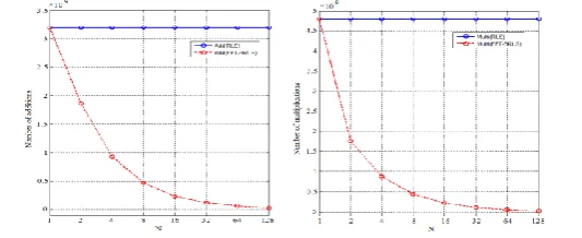
4.2. Calculation Complexity

This section is devoted to the study of the computational complexity of three adaptive algorithms: RLS, Toeplitz-BRLS and FFT-BRLS. We will present the number of operations (additions, multiplications, subtractions and divisions) necessary to implement the three algorithms in question.

As mentioned in paragraph 2.2.2, the number of additions/subtractions and multiplications/divisions implemented for the RLS algorithm at each iteration k, _is respectively of the order

2

L

2



1

,

and 3L27L. _{Consequently,}

for processing the echo signal of our study, which is composed of

97408samples, this algorithm needs 97408iterations.

The FFT-BRLS algorithm requires two convolution products as shown in the two equations (21) and (22). The computation of each convolution product requires the computation of three transforms, two direct (FFT) and one

inverse



FFT

1



.

The number of additions and multiplications implemented for a FFT or for one _FFT1 _{is of the order of}

M

Mlog_{2 and}

₂

log

2

M

,

M

The figure (7) provides a comparison in terms of the number of additions and multiplications necessary for the implementation of the two adaptation methods, RLS and FFT-BRLS as a function of

N

.

_{This comparison is carried out from a sequence}

of length

M



256

.

Figure 7. Computation complexity of two RLS and FFT-BRLS algorithms as a function of N and for L = 128

The curves show that, as N increases, the number of calculations decreases for the FFT-BRLS algorithm, and the more the benefit of FFT implementation will be marked. If N = 1, this corresponds to the RLS algorithm. In this particular case where N = 1, the FFT-BRLS algorithm has the same number of operations as that of the RLS algorithm.

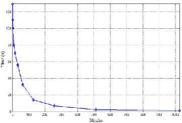
4.3. Execution Time

The performance of the block-processed RLS algorithm is intended to compare this time the execution time of both the RLS and the FFT-BRLS algorithms to highlight the advantage of using the block processing method using the Fast Fourier transform (FFT). In this comparison, the length of the blocks varies between N=1 (this is the particular case that corresponds to the RLS algorithm) and N=1024. The figure (8) shows an example of this comparison.

the reduction of the execution time is observed when N increases. On the other hand, the execution time represented by the RLS algorithm is generally the same, is equal to t = 129.15 seconds in order to process 97408 samples (number of samples of the echo signal).

Figure 8. Execution time of the FFT-BRLS algorithm as a function of N

5. CONCLUSION

computational complexity by implementing the Fast Fourier Transform (FFT).

The results of the simulations reveal no noted difference in terms of convergence between the two adaptation methods (sample processing represented by the RLS algorithm and block processing). The only difference between the two methods resides in the computational complexity and the execution time, which was reduced by the new FFT-BRLS algorithm.

REFERENCES

1. [Gilloire 1987] Gilloire A., and Julien J.P. (1987). L’acoustique des salles dans les télécommunications. L’écho des recherches, n° 127, p. 43-54.

2. [Kazuo 1990] Kazuo M, Shigeyuki U, and Fumio A (1990). Echo Cancellation and Applications. IEEE Communications Magazine, p.49-55.

3. [Farhang 1998] Farhang-Boroujeny B (1998). Adaptive Filters. Theory and Apllications. Wiley & Sons, ISBN 978-0-471-98337-8.

4. [George 1999] George-Othon G, Kostas B, and Sergios T (1999). Efficient Least Squares Adaptive Algorithms for FIR Transversal Filtering. IEEE Signal Processing Magazine, p. 13-41.

5. [Paleologu 2010] Paleologu C, Benesty J, and Ciochina S (2010). Sparse Adaptive Filters for Echo Cancellation. Morgan & Claypool Publishers,

6. [Ljung 1983] Ljung L and Söderström T (1983). Theory and Practice of Recursive Identification. M.I.T.Press.

8. [Gilloire 1994] Gilloire A, and Vetterli M (1994). Performance evaluation of acoustic echo controls: required values and measurement procedures. Annales des Télécommunications. vol 49, n°7, p. 368-372.

9. [Clark 1981] Clark G.A, Mitra S.K, and Parker S.R (1981). Block implementation of adaptive digital filters. IEEE Trans. on Circuits and Systems. vol. CAS-28, p. 585-592. 10.[Alaeddine 2012] Alaeddine H, Bazzi O, Alaeddine A,

Mohanna Y and Burel G (2012). Fast convolution using generalized sliding Fermat number transform with application to digital filtering. Journal of The Institute of Electronics, Information and Communication Engineers (IEICE), E95-A (6), p.1007-1017.

11.[Khong 2005] Khong A, Benesty J, and Naylor P.A (2005). An improved proportionate multi-delay block adaptive filter for packet-switched network echo cancellation, in Proc. EUSIPCO Actes du colloque Sémio 2005, Antalya, Turkey.

APPENDIX: RECURSIVE LEAST SQUARES (RLS) ALGORITHM

We will develop a recursive algorithm which, using the coefficients of

the filter at the instant k1, will estimate these coefficients at the instant using the new available data.

Problem Statement

Our objective is to estimate the parameters wˆk using the following

least squares criterion:











 

k

n n

T k n n k

k

d

w

x

0

2

ˆ





(A.1)

With



is a weighting factor that always takes a positive value: 0

. 1



forget data that corresponds to a distant past. The particular case

1





_{corresponds to an infinite memory.}

The normal equations

The problem is to determine the vector of the coefficients wˆkwhich

minimizes



k.The solution is obtained by calculating the derivatives

of the cost function



k and by equating them to zero:











 



k

n n n L

T k n n k

x

x

w

d

0 1

0

ˆ



(A.2) Let:

 







    k n k T n n k n n k n n n k

w

x

x

x

d

0 0

ˆ





(A.3) It then comes:

k k

k w

Q  ˆ _(A.4)

k k

k

Q

w

ˆ





1 _(A.5) With:







  k n T n n n k

k

x

x

0



(A.6) n n k n n k

k d x

Q





 

0



(A.7) The above equations can be computed recursively

T k k k

k







x

x





_{1 (A.8)}

We have also:

k k k

k Q d x

Q  1 (A.9)

RLS algorithm

It is recalled that the correlation matrix is:

T k k k

k







x

x





_{1 (A.10)}

The inversion lemma can be used to compute the inverse of k, let: ,

k

A

B

1







_k1,Cx_{kand D}₁

Thus we obtain the following recursive equation for the inverse of the correlation matrix: k k T k k T k k k k k

x

x

x

x

1 1 1 1 1 1 1 2 1 1 1 1

1

 _

        























(A.11) Let: 1 



 _k k

P _and k k

T k k k k

x

P

x

x

P

G 1 1 1 1

1

 _

 









(A.12)

Then the recursive equation for Pk can again be written:

1 1 1 1     _

 T _k

k k k

k P

G

x

P

P





_(A.13)

The vector Gk is called Kalman gain, which can be rearranged: k

k

k P x

G  _(A.14)

Now, we need to compute the filter coefficients recursively. We have:

k k k k k k k k k

k Q P Q P Q P x d

wˆ 1   _1 _(A.15)

By replacing Pk in the first term of the preceding expression by

equation (A.13), we obtain:



1



1 1 1 1 1 ˆ ˆ ˆ             k T k k k k k k k k k T k k k k k w x d G w d x P Q P G Q P w x (A.16) Finally, we have:

k k k

k w G e

wˆ  ˆ _1 _(A.17)

Where

1

ˆ _





T _k

k k k

d

x

w

e

_(A.18) is the a priori error that is different from the posterior error:

k T k k k

d

x

w

e





ˆ _(A.19)