A New Algorithm for Protein-Protein Interaction Prediction

Scholarship@Western

Scholarship@Western

Electronic Thesis and Dissertation Repository

12-18-2013 12:00 AM

A New Algorithm for Protein-Protein Interaction Prediction

A New Algorithm for Protein-Protein Interaction Prediction

Yiwei Li

The University of Western Ontario Supervisor

Dr. Lucian Ilie

The University of Western Ontario

Graduate Program in Computer Science

A thesis submitted in partial fulfillment of the requirements for the degree in Master of Science © Yiwei Li 2013

Follow this and additional works at: https://ir.lib.uwo.ca/etd Part of the Other Computer Sciences Commons

Recommended Citation Recommended Citation

Li, Yiwei, "A New Algorithm for Protein-Protein Interaction Prediction" (2013). Electronic Thesis and Dissertation Repository. 1841.

https://ir.lib.uwo.ca/etd/1841

This Dissertation/Thesis is brought to you for free and open access by Scholarship@Western. It has been accepted for inclusion in Electronic Thesis and Dissertation Repository by an authorized administrator of

A NEW ALGORITHM FOR PROTEIN-PROTEIN INTERACTION

PREDICTION

(Thesis format: Monograph)

by

Yiwei Li

Graduate Program in Computer Science

A thesis submitted in partial fulfillment

of the requirements for the degree of

Masters of Science

The School of Graduate and Postdoctoral Studies

The University of Western Ontario

London, Ontario, Canada

c

Protein-protein interactions (PPI) are vital processes in molecular biology. However, the current understanding of PPIs is far from satisfactory. Improved methods of pre-dicting PPIs are very much needed. Since experimental methods are labour and time consuming and lack accuracy, the improvement is expected to come from the area of computational methods.

We designed and implemented a new algorithm based on protein primary structure to predict PPIs using C++ and OpenMP for parallel computing. We compared our method with four leading methods. Our results are better than the competition for most of the important values. Furthermore, it succeeds in surpassing the consensus of the other methods.

Acknowlegements

First of all, I would like to show my sincere appreciation to my supervisor, Dr. Lucian Ilie. The most important thing I learned from him is never stop thinking. Without his insightful guidance and late-night video chatting, I could not finish this thesis.

Second, I would like to show my gratitude to my parents. Thank you for your 24-year support and love.

Finally, my heartfelt appreciation goes to all my lab-mates, especially Ehsan Haghshenas, a good colleague, friend, and roommate who helps me a lot.

Certificate of Examination ii

Abstract ii

List of Figures vi

List of Tables viii

1 Introduction 1

2 Background 4

2.1 Molecular biology primer . . . 4

2.2 Proteins, domains, and interactions . . . 6

2.3 Experimental approaches . . . 8

2.3.1 Yeast two-hybrid (Y2H) . . . 8

2.3.2 Tandem affinity purification (TAP) . . . 9

2.4 Computational approaches . . . 10

2.5 Leading programs . . . 15

2.5.1 Method 1 . . . 15

2.5.2 Method 2 . . . 15

2.5.3 Method 3 . . . 16

2.5.4 Method 4 . . . 19

3 A new algorithm 21 3.1 Domains are responsible for interactions . . . 21

3.3 Detecting domains as similarities . . . 24

3.4 Scoring domain pairs . . . 29

3.5 Predicting PPIs . . . 31

3.6 Improving the results . . . 31

4 Evaluation 35 4.1 Datasets . . . 35

4.2 Competing programs . . . 36

4.3 Comparison . . . 37

5 Conclusion 42

Bibliography 43

Curriculum Vitae 47

2.1 Transcription and Translation. From: tokresource.org . . . 5

2.2 Protein sequence. From: wikimedia.org . . . 5

2.3 A protein in FASTA format. . . 6

2.4 The protein-protein interaction network of human. From: www.mdc-berlin.de . . . 7

2.5 Domain-Domain Interaction. From: [31] . . . 8

2.6 The Y2H approach. From: [42] . . . 9

2.7 Tandem affinity purification. From: [15] . . . 10

2.8 Genomic approach. From: [15] . . . 11

2.9 Phylogenetic profiles approach. From: [15] . . . 12

2.10 Protein structure approach. From: [15] . . . 13

2.11 Domain based approach. From: [15] . . . 13

2.12 Network analysis approach. From: [15] . . . 14

2.13 Algorithm of PIPE. From: [30] . . . 17

2.14 Constructing the vector space (V, F) of a protein sequence. From: [38] . 18 2.15 Classification of amino acids. From: [38] . . . 18

2.16 Representation of each amino acid . . . 19

2.17 Values of the seven physicochemical properties for each amino acid. From supplementary material of [10] . . . 20

3.2 Consecutive seed (left) and spaced seed (right). The red 1’s are new matches required for a hit at the next position; it is much easier for the consecutive seed to have consecutive hits, hence its hits are more clustered

than those of the spaced seed. . . 23

3.3 The BLOSUM80 matrix . . . 24

3.4 Extractings-mers. . . 26

3.5 Domain merging. The red and blue occurrences overlap and become a single occurrence of the same domain . . . 30

3.6 Splitting domain. . . 32

4.1 Cross validation. . . 36

4.2 Binary classification. From [7] . . . 37

4.3 Discrete classifiers in ROC curve. From [7] . . . 38

4.4 Generating ROC points. From [7] . . . 38

4.5 Fawcett’s fast algorithm for generating ROC curves. From [7] . . . 39

4.6 ROC curve comparision with other four methods . . . 40

4.7 ROC curve comparision with consensus method . . . 41

3.1 Amino acid encoding . . . 25

Chapter 1

Introduction

Proteins are essential molecules in organisms. It is quite often that proteins perform their functions by interacting with other proteins, binding into a stable or temporary complex. It is reported that humans have a similar number of genes with a worm [44], which implies that the differences between organisms are not solely given by the protein numbers, but also by the relations between proteins. A more complicated protein-protein interaction network makes an organism like human more sophisticated.

Currently, the understanding of protein-protein interaction (PPI) networks is far from satisfactory. Even for very small organisms, the ratio between known and potential PPIs is about 1:500 [15, 40]. Obtaining a more complete PPI network for different organisms would help to identify proteins that have the same functions. Additionally, we can have a broader view of which proteins interact more often or with what kinds of other proteins. Therefore, a significant amount of research has been done in the area of protein-protein interaction prediction. Both experimental and computational methods have been developed.

Yeast two-hybrid (Y2H) [8] and tandem affinity purification (TAP) [32] are two widely used experimental methods. Y2H attaches DNA-binding domains (DBD) and activation domains (AD) to proteins, and tell whether a pair of proteins interact or not by detecting a reporter generated by DBD and AD. The TAP method detects protein interaction complexes by adding a “tag” to that complex. After tandem affinity purification, all proteins involved are assumed to interact.

Though experimental methods can make valuable predictions, they are labour and time consuming. In addition, their false positive and false negative rates are high.

Due to the limitations of experimental methods, many types of computational meth-ods have been proposed. Genomic methmeth-ods [27] detect PPIs by detecting gene neighbour-hood conservations, evolutionary relationship methods [27, 44] use phylogenetic profiles, protein structure methods [23, 18, 39] use 3D structures of proteins to find docking areas, domain methods [6] employ conserved domain occurrences, network analysis methods [4] make prediction possible using graph theory and machine learning, and primary protein structure methods [4, 24, 44, 24, 30, 38, 10] use protein sequences, usually along with machine learning techniques.

Although computational methods have advantages over experimental methods, most of them are still inefficient and can not run the whole proteome of advanced organisms like human within an affordable time.

Among those computational methods, four leading methods have being widely used. The algorithm of Martin et al. [24] uses support vector machines (SVM) on signature products, PIPE [30] computes a prediction matrix based on similarities between proteins, Shen et al. [38] use SVM and kernel functions, and Guo et al. [10] employs covariance as the input of SVM.

Park [26] evaluated the above mentioned four methods and implemented a consensus method which integrated all four. The result of the consensus method outperforms all other four methods consistently, which implies a high possibility for designing a more reliable program.

We designed and implemented a new sequence-based PPI prediction algorithm. We compare our program with the four programs in Park’s paper. Our method is better than the others for most of the important values. Moreover, for a good part, it succeeds in surpassing the consensus of the other methods.

Background

This chapter introduces some prerequisite knowledge in molecular biology. Then basic concepts of protein interactions are provided. Protein-protein interaction prediction can be done by both experimental and computational approaches. Both types are introduced, and four leading computational programs are described.

2.1

Molecular biology primer

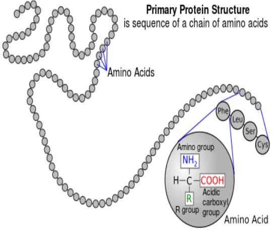
DNA is the code of life. All living organisms are coded by four nucleotides: adenine (A), thymine (T), guanine (G), and cytosine (C). DNA has a double helix structure which is composed of sugar molecules, phosphate group, and bases (A, G, C, T). In DNA strands, A is always matched with T and G is always matched with C ([16]).

DNA can copy itself via replication. It can also transcript into RNA. During tran-scription, the information in DNA pairs is passed to corresponding RNA, which will use uracil (U) instead of thymine (T) to match adenine. After transcription, RNA will be translated into protein. In the process of transcription, every three nucleotides (codon) will determine one kind of amino acid. A string of amino acids forms one kind of protein. Figure 2.1 shows the transcription and translation process in a cell. Figure 2.2 shows a protein sequence.

Proteins are made of twenty kinds of amino acids. The function of proteins varies. The main functions of proteins can be working as antibodies, contractile proteins,

2.1. Molecular biology primer 5

Figure 2.1: Transcription and Translation. From: tokresource.org

Figure 2.2: Protein sequence. From: wikimedia.org

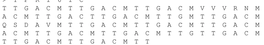
> Y P R 1 6 1 C

T T G A C M T T G A C M T T G A C M V V V R N M A C M T T G A C T T G A C M T T G M T T G A C M Q S D A V M T T G A C M T T G A C M T T G A C M A C M T T G A C M T T G A C M T T G T T G A C M T T G A C M T T G A C M T T

Figure 2.3: A protein in FASTA format.

A FASTA file consists of protein or DNA names, description and sequences. Identifiers are preceded by a greater-than symbol “>” and the rest of the line is a description (optional). The next lines up to the next greater-than symbol contain the actual DNA or protein sequence. Figure 2.3 shows an example of a FASTA format. The protein name “YPR161C” follows the “>” sign. The protein sequence is given in the next five lines.

2.2

Proteins, domains, and interactions

The proteins are some of the most important molecules in cells ([34]). They carry out most of the cellular processes. Quite often, they keep the cells functioning by interacting with other proteins in stable or transient protein complexes ([5]). This process is called protein-protein interaction (PPI). This is a vital process because of the accepted idea that PPIs are responsible for cell’s behaviour and different stimuli ([2, 25, 35]). From this point of view, scientists believe the reason that advanced organisms like humans are more complicated than lower organisms like the worms is not only because of large number of genes, but also because of sophisticated PPI networks [29]. Figure 2.4 shows the map of human PPI network. Understanding the potential of unknown proteins is becoming possible by looking into their PPI infomation [37]. As well, knowing PPI information helps improve the system-level understanding of molecular processes [19]. Therefore, understanding and mapping PPIs is an important current area of research.

2.2. Proteins, domains, and interactions 7

Figure 2.4: The protein-protein interaction network of human. From: www.mdc-berlin.de

where a part of one protein complements a part of another protein.

One commonly accepted assumption is that the same domain in different proteins functions the same, and protein-protein interactions are conducted via domain-domain interactions (DDIs) [43]. Thus, finding the conserved similar domains in each protein would help understand PPIs. Also, based on DDIs, we can design computational methods to predict PPIs.

Figure 2.5: Domain-Domain Interaction. From: [31]

2.3

Experimental approaches

Some widely known experimental approaches are designed and employed by biologists. Two of them will be briefly introduced in this section, yeast two-hybrid (Y2H) and tandem affinity purification (TAP).

2.3.1

Yeast two-hybrid (Y2H)

The yeast two-hybrid (Y2H) approach was proposed by Suter et al. [8]. It detects a protein interaction by telling the signal generated by the DNA-binding domain (DBD) and the activation domain (AD) [42].

2.3. Experimental approaches 9

Figure 2.6: The Y2H approach. From: [42]

Although Y2H is able to detect many protein-protein interactions, the drawbacks of this approach are obvious. First, it can only detect PPIs within the nucleus. Second, it can only detect one interaction at a time, which is quite inefficient. Also, the false positive and false negative rates are high [41, 36].

2.3.2

Tandem affinity purification (TAP)

Another widely used experimental approach is tandem affinity purification, which was invented by Rigaut et al. [32]. It can detect protein complex interaction by adding a “tag” to target proteins.

Figure 2.7 shows the general process of TAP. If we want to test whether interaction exists between protein A and proteinB, a tag is added to protein A. After tagging, the complex is washed twice to remove the tag and unstable bindings. Isolated interacting proteins can be found if there are some. After washing, the mass spectrometry or other methods will be used to detect remaining proteins. The remaining ones are marked as interacting proteins [32].

Figure 2.7: Tandem affinity purification. From: [15]

a way that changes the interacting process. Also, some real interactions can be washed away during two times of washing, thus increasing the false negative rate [15].

2.4

Computational approaches

The experimental approaches are time and labour consuming. Also, they have the limi-tation of being unable to detect some protein complexes. In addition, the false positive rate and false negative rate of those approaches are high ([30]).

Due to the limitations of experimental approaches, we have imperative demanding for efficient, affordable, and more precise computational approaches.

Currently, there are mainly six kinds of computational PPI prediction approaches: ge-nomic approach, evolutionary relationship approach, protein structure approach, domain approach, network analysis approach, and primary protein structure approach [15].

2.4. Computational approaches 11

genomes are predicted to interact (gene neighbourhood conservation) [27, 44]. In Figure 2.8, there are four different genomes, A, B, C, and D. Proteins 1, 2, and 3 appear in those genomes, and we can predict that protein 1 will interact with protein 2 because in genomes A, B and D, their genes occur in close physical proximity [15].

Figure 2.8: Genomic approach. From: [15]

Phylogenetic profiles approach suggests that during the process of evolution, inter-acting pairs of proteins will be preserved in order to function together ([27, 44]). Figure 2.9 shows four proteins along with their phylogenetic profiles in four genomes. The inter-action between protein 1 and protein 4 can be predicted because both appear in genome A and genome D ([15]).

Figure 2.9: Phylogenetic profiles approach. From: [15]

Protein structure approach uses techniques such as X-ray crystallography or NMR spectroscopy to obtain 3D structure of proteins. If two proteins are homologous and share similar sequence, they should interact in a similar way ([23, 18, 39]).

Figure 2.10 shows a simple model of predicting PPIs using protein structure approach. Protein 1 and protein 4 are predicted to be interacting since the docking parts of those proteins fit the best [15].

Domain based approach detects occurrences of sub-sequences (domain) in a protein sequence. It is accepted that protein-protein interactions happen via domain-domain interactions. If conserved domains are found, we can use those domains to predict new interactions [6].

In Figure 2.11, protein A and protein B are a known interacting pair. Domain 1 and domain 2 are estimated as conserved domains. We predict that proteinC and protein D

interact because protein C contains a region that is similar to domain 1 and protein D

contains a region is similar to domain 2 ([15]).

2.4. Computational approaches 13

Figure 2.10: Protein structure approach. From: [15]

sub-graph can form a clique ([15]).

Figure 2.12: Network analysis approach. From: [15]

Figure 2.12 shows an simple instance of network analysis approach. Each node denotes a protein and each solid line denotes a known interaction between two proteins. Proteins

A, B, C and D can form a clique by adding the edge A-C. So we predict that proteins

A and C interact.

An advantage of network analysis approach is that we can visually see the interaction network. We can tell the connections of a certain protein. We can tell as well how often a protein interacts with others. The detailed algorithm is more complicated than simply adding edges, otherwise the false positive rate would be too high [15].

The primary protein structure approach is proposed under the hypothesis that PPIs are conducted via polypeptide sequences. They usually use machine learning techniques such as support vector machines (SVM) or Random Forest (RF) to find binding regions of PPIs ([4, 24, 44]).

2.5. Leading programs 15

2.5

Leading programs

Despite the fact that many computational approaches have their own advantages com-paring with experimental ones, most of them are too expensive regarding computation time. They cannot run on the entire human proteome because it takes unreasonably long time [15]. Park [26] published an assessment of the current leading PPI prediction methods. He compared in details four leading computational methods.

The characteristics of these four methods is that they are all sequence based (no evolutionary information required). Those four methods are described below. Our own method will be compared with those later.

2.5.1

Method 1

Martin et al. [24] proposed a predicting method using signature products. In this method, an amino acid sequence is represented as a signature, which is a combination of three letters. For example, the amino acid sequence LVMTTM, trimers are: LVM, VMT, MTT and TTM. They are made of a root (middle letter) and two neighbours (side letters). Then the signatures of those trimers are V (LM), V (MT), T (MT), T (MT), respectively. By adding those vectors together, the signature of the sequence is V (LM) + V (MT) + 2T (MT) [24]. Note that 2T(MT) comes from T(MT) + T(TM).

The signature will be classified by support vector machines (SVM). Then, using ma-chine learning methods, predictions will be made.

2.5.2

Method 2

The Protein-protein Interaction Prediction Engine (PIPE) series was initiated by Pitre et al. [30]. It is one of the most widely known methods. PIPE can successfully predict new interactions based on re-occurring short sub-sequences in an existing interaction database. The major four steps of PIPE are shown in Figure 2.13. Given an interaction database, an interaction graph (G) is built. Given a query protein pair (A, B), a window

w is first slid across A and, for each position, the peptide ai in the window is searched

similar withai are stored in a listR of neighbours. In Figure 2.13, proteinsV and W are

hit and their neighbours,X, Y, Z, are added toR. A similar window is then slid across

B and any time a neighbour from R is hit, that is, it is found to contain a sequence similar to the current window content bj, a counter for (ai, bj) is incremented, where ai

is the initial segment of A that was used to find the neighbour in R. This way a matrix is obtained, whose (i, j) value is the counter for (ai, bj) mentioned above. The highest

score of that matrix (if higher than a threshold) is where interaction most likely happens between proteinsA and B ([30]). In Figure 2.13, this procedure finds a sub-sequences in

A that is similar with, V, for example. Meanwhile, a sub-sequences of B is similar with a sub-sequences of X, SinceX and V interact, we predict, based on highest score in the matrix, that the same conserved interaction will happen as well between A and B.

The second version of PIPE was published in 2008 [28]. The improvement of this version is the increase of sensitivity and reduction of running time. Also, prediction of whole yeast proteins are made possible in this version.

PIPE3 changes the architecture to parallel and reduces the memory usage so that it can predict human protein-protein interactions, though it still takes a very long time. On 50 nodes, and a total of 12,800 multiple threads, prediction on human proteome will take more than three months using PIPE3.

2.5.3

Method 3

Shen et al. [38] proposed a sequenced-based PPI prediction method. This method uses also machine learning techniques to make predictions. Their program uses protein sequences and PPIs as training data. Then it classifies new pairs of proteins with support vector machines (SVM) and a kernel function.

SVMs are used for classifying PPIs into two different sets, interacting or non-interacting. The kernel function is used for mapping training data into a higher dimension, in order to classify it linearly. A detailed introduction about SVM and kernel function can be found for instance in [11].

2.5. Leading programs 17

Figure 2.13: Algorithm of PIPE. From: [30]

three amino acids are grouped as a vector space (V, F), where V is the encoded value, from 1 to 343, and F is the frequency with which those three amino acids appear. For example, the first three amino acids are encoded as (342, 1), because this combination has only appeared once. The 20 amino acids are classified into 7 classes based on the dipoles and volumes of side chain. A detailed classification is shown in Figure 2.15.

Figure 2.14: Constructing the vector space (V, F) of a protein sequence. From: [38]

2.5. Leading programs 19

2.5.4

Method 4

Guo et al. [10] proposed another PPI prediction approach. This method uses SVMs and auto covariance (AC) to make predictions.

Similarly with the methods mentioned in 2.5.1 and 2.5.3, SVMs are used for classifying new pairs of proteins into interacting or non-interacting sets. Each amino acid in a protein sequence is represented as neighbouring effects and physicochemical properties (shown in Figure 2.16). According to their optimization experiment, for each amino acid, they take into account 30 neighbour amino acids of it. This neighbouring effect is then translated into a numerical value. The physicochemical properties of each amino acids are shown in Figure 2.17 where H1 = hydrophobicity, H2 = hydrophilicity, V = volume of side chains, P1 = polarity, P2 = polarizability, SASA = solvent accessible surface area, NCI = net charge index of side chains. Variables of neighbouring effect and physicochemical properties be will used to calculate AC variables. SVM will take these AC variables as input to make predictions.

Chapter 3

A new algorithm

Our new algorithm to predict PPIs, based on protein sequence only, is described in this chapter. It is implemented in C++ and uses OpenMP for parallelization.

3.1

Domains are responsible for interactions

As discussed in Chapter 2, domain-domain interactions (DDIs) imply protein-protein interactions (PPIs). And because one domain can appear in different proteins, the same DDI can happen between different interacting protein pairs.

Since protein interactions are essential to protein functions, they have to be well preserved during evolution. It is therefore expected that the domains responsible for these interactions are preserved as well. Indeed, it is the 3D structure that requires conservation, but that implies that the amino acid structure should be well conserved as well. That means that different occurrences of the same domain should have a high degree of sequence similarity. Therefore, our starting point will be sequence similarity identification.

The main steps of the algorithm are shown below:

• Detect similarities

• Identify domains

• Attach scores to domain pairs

• Attach scores to protein pairs

• Predict PPIs

3.2

Spaced seeds

Our first problem is finding the similar sub-sequences within protein sequences of an or-ganism. The classic similarity search tool is BLAST (Basic Local Alignment Search Tool) [1]. The basic idea of BLAST is called “hit and extend”. When identifying similarity, BLAST requires several consecutive matches between two strings; the default number for DNA is 11 consecutive matches. Denoting the matches by 1’s we obtain what is called a consecutive seed: 11111111111. A pair of identical consecutive matches is called a hit.

Figure 3.1 shows the basic idea of BLAST. When a hit is detected by the consecutive seed, marked with red color, BLAST extends this hit towards both sides. If the score increases, it continues extending. If the score drops below a threshold, it stops. The blue part is where BLAST extends.

| ← h i t → |

T T G A C A T G T C T C T A G T G A G T C T C T A T | | | | | | | | | | | | | | | | | | | |

T T A C T A T G T C T C T A G T G A G T C T C A T G 1 1 1 1 1 1 1 1 1 1 1 1

| ← ext. ext. → |

Figure 3.1: Hit and extend in BLAST.

3.2. Spaced seeds 23 C G T C A A G A C T T ? G A G ? C ? ? T ?G ? ? A C? T T C ?

| | | | | | | | | | | ? | | | ? | ? ? | ?| ? ? | |? | | | ?

C G T C A A G A C T T ? G A G ? C ? ? T ?G ? ? A C? T T C ? 1 1 1 1 1 1 1 1 1 1 1 _{1 1 1 * 1 * * 1 * 1 * * 1 1 * 1 1 1}

1 1 1 1 1 1 1 1 1 1 1 1 11 _* 1_{* *} 1_* 1 _{* * 1} 1 _{* 1 1} 1

Figure 3.2: Consecutive seed (left) and spaced seed (right). The red 1’s are new matches required for a hit at the next position; it is much easier for the consecutive seed to have consecutive hits, hence its hits are more clustered than those of the spaced seed.

While consecutive seeds suffer form hit clustering (Figure 3.2 left), spaced seeds have their hits much better distributed (Figure 3.2 right). The number of 1’s in a seed defines the weight of the seed, whereas 1’s and *’s together are its length. The probability of a hit depends only on the weight of the seed. Therefore, two seeds, one consecutive and one spaced, of the same weight have the same number of expected hits. Because the hits of a spaced seed are less clustered together, more regions will be hit, thus increasing the probability of finding similarities. This probability is called the sensitivity of the seed.

Using several spaced seeds [20] dramatically improves sensitivity. The only problem is that computing optimal seeds is a hard problem. Even the heuristic algorithms are exponential, except for SpEED [13, 14]. We have thus used SpEED to compute the mul-tiple spaced seeds to be used in our PPI prediction program. They are given below: seed1 = 11*111

seed2 = 111**1*1

seed3 = 11***1*11

seed4 = 1*1***111

seed5 = 1*1*1**11

seed6 = 11*****1*11

seed7 = 11*1**1***1

3.3

Detecting domains as similarities

After having computed the seeds, we need to find a way to detect domains fast. In agreement with other methods, we are going to use BLOSUM80 [12] as our similarity matrix (see Figure 3.3).

A R N D C Q E G H I L K M F P S T W Y V A 5 -2 -2 -2 -1 -1 -1 0 -2 -2 -2 -1 -1 -3 -1 1 0 -3 -2 0 R -2 6 -1 -2 -4 1 -1 -3 0 -3 -3 2 -2 -4 -2 -1 -1 -4 -3 -3 N -2 -1 6 1 -3 0 -1 -1 0 -4 -4 0 -3 -4 -3 0 0 -4 -3 -4 D -2 -2 1 6 -4 -1 1 -2 -2 -4 -5 -1 -4 -4 -2 -1 -1 -6 -4 -4 C -1 -4 -3 -4 9 -4 -5 -4 -4 -2 -2 -4 -2 -3 -4 -2 -1 -3 -3 -1 Q -1 1 0 -1 -4 6 2 -2 1 -3 -3 1 0 -4 -2 0 -1 -3 -2 -3 E -1 -1 -1 1 -5 2 6 -3 0 -4 -4 1 -2 -4 -2 0 -1 -4 -3 -3 G 0 -3 -1 -2 -4 -2 -3 6 -3 -5 -4 -2 -4 -4 -3 -1 -2 -4 -4 -4 H -2 0 0 -2 -4 1 0 -3 8 -4 -3 -1 -2 -2 -3 -1 -2 -3 2 -4 I -2 -3 -4 -4 -2 -3 -4 -5 -4 5 1 -3 1 -1 -4 -3 -1 -3 -2 3 L -2 -3 -4 -5 -2 -3 -4 -4 -3 1 4 -3 2 0 -3 -3 -2 -2 -2 1 K -1 2 0 -1 -4 1 1 -2 -1 -3 -3 5 -2 -4 -1 -1 -1 -4 -3 -3 M -1 -2 -3 -4 -2 0 -2 -4 -2 1 2 -2 6 0 -3 -2 -1 -2 -2 1

F -3 -4 -4 -4 -3 -4 -4 -4 -2 -1 0 -4 0 6 -4 -3 -2 0 3 -1 P -1 -2 -3 -2 -4 -2 -2 -3 -3 -4 -3 -1 -3 -4 8 -1 -2 -5 -4 -3 S 1 -1 0 -1 -2 0 0 -1 -1 -3 -3 -1 -2 -3 -1 5 1 -4 -2 -2 T 0 -1 0 -1 -1 -1 -1 -2 -2 -1 -2 -1 -1 -2 -2 1 5 -4 -2 0 W -3 -4 -4 -6 -3 -3 -4 -4 -3 -3 -2 -4 -2 0 -5 -4 -4 11 2 -3

Y -2 -3 -3 -4 -3 -2 -3 -4 2 -2 -2 -3 -2 3 -4 -2 -2 2 7 -2 V 0 -3 -4 -4 -1 -3 -3 -4 -4 3 1 -3 1 -1 -3 -2 0 -3 -2 4

Figure 3.3: The BLOSUM80 matrix

We encode each amino acid with 5 bits. Blocks of 5 bits can have 25 _{= 32 different}

3.3. Detecting domains as similarities 25

Amino acid name Notation in FASTA format 5-bit encoding Alanine A 00000 Arginine R 00001 Asparagine N 00010 Aspartic acid D 00011 Cysteine C 00100 Glutamine Q 00101 Glutamic acid E 00110 Glycine G 00111 Histidine H 01000 Isoleucine I 01001 Leucine L 01010 Lysine K 01011 Methionine M 01100 Phenylalanine F 01101 Proline P 01110 Serine S 01111 Threonine T 10000 Tryptophan W 10001 Tyrosine Y 10010 Valine V 10011

Table 3.1: Amino acid encoding

The eight seeds will be encoded as eight unsigned 64-bit integers. In a spaced seed, “1” is encoded as “11111” in 5 bits, while “0” is encoded as “00000”. For instance, the seed “11010011” is encoded as “11111 11111 00000 11111 00000 00000 11111 11111” in an unsigned 64-bit integer. The longest seed has length 11, which will fit into 55 bits.

For a seed s, an s-mer is a sequence of amino acids interspersed with spaces, of the same length as the seed, such that the amino acids correspond to the 1 positions in s. For instance, if the seed is s= 11010011, than ans-mer could be MF E NF. Spaces are implemented as 0’s, so this s-mer is in fact MF0E00NF. Similar to the consecutive case, a hit consists of a pair of sub-sequences that match to the positions corresponding to the 1’s in the seed (see again Figure 3.2 right); that is, matching s-mers. Therefore, we need a fast way of extracting the s-mers from protein sequences.

example how seed 11010011 is extractings-mers from a protein sequence. The 0 position will always extract 0 because 0 means don’t care. Amino acids in other positions (1’s in seed) will be extracted as in the original sequence. So, for the sequence “MFSELIN-FQNEG”, the seed “11010011” will extract the first s-mer “MF0E00NF”. After shifting one position, the second s-mer “FS0L00FQ” will be extracted.

M F S E L I N F Q N E G 1 1 0 1 0 0 1 1

M F 0 E 0 0 N F

→ 1 1 0 1 0 0 1 1

→ F S 0 L 0 0 F Q

→ 1 1 0 1 0 0 1 1

→ S E 0 I 0 0 Q N

. . .

Figure 3.4: Extracting s-mers.

The way we extract s-mer is doing “bitwise and” for encoded seed and encoded proteins. In this way, one “and operation” will extract a wholes-mer from the sequence. It is much faster than using characters or strings.

As mentioned earlier, finding similar sub-sequences start with finding hits, that is, matching s-mers. In order to do this fast, we use a hash table. All extracted s-mer will be stored in the hash table. For each seed, we have one hash table. The hash function is:

entry index=s mer value % hash size (3.1)

where the hash size is determined when encoding proteins. For each seed, the maxi-mum number of s-mers is:

number of smers=

num of pro

X

i=1

(protein length−seed length+ 1).

3.3. Detecting domains as similarities 27

protein ids and starting positions of thats-mer. The pseudocode for computing the eight hash tables is given in Algorithm 1. Algorithm 2 shows the insertion into hash table in detail. We use OpenMP to parallel this part so that eight hash tables can be built simultaneously.

Algorithm 1: Algorithm for computing hash tables

input : encoded proteinsEP, 8 encoded seeds S output: 8 hash tables HT

1 for each seed s∈S do

2 - initialize ht ∈HT

3 - for each protein p∈EP do

4 - temp protein sequence =p

5 - for position∈[0,(pro length−seed length+ 1)] do 6 - s-mer = s &temp protein sequence

7 - temp protein sequence shift one position

8 - insert into hash table (s-mer, position, ht)

9 end

10 end

11 end

Algorithm 2: Algorithm for inserting s-mer into hash table

input :s-mer, s-mer position, hash table output:

1 position p =s-mer %hash size 2 if hash table[p] == ∅then

3 insert (s-mer, s-mer position) into hash table[p] 4 end

5 else if s-mer ==hash table[p].s-mer then

6 add (s-mer position) into hash table[p] as a linked list 7 end

8 else if s-mer 6=hash table[p].s-mer then

9 insert s-mer into hashtable(s-mer, p + 1, hash table) 10 end

After having the eight hash tables, we start investigating hits as indicated by Algo-rithm 3. For every s-mer x in the hash table, we compute all s-mers y that are similar enough to x. Here similar enough means that the score between x and y is greater than

Thit (hit threshold). The score between two strings of the same length is computed as

our case, BLOSUM80. That is, if x=x1x2...xn, y=y1y2...yn, then

score(x, y) =

n

X

i=1

scoreB80(xi, yi) (3.2)

Algorithm 3: Algorithm for investigating hits

input : eight seeds and corresponding hash tables

output: a record of domains in each protein

1 for each seed s∈S do

2 for each s-mer x do

3 compute H(x) = {y | y > x, score(x,y)> T_hit } (Algorithm 4) 4 for all y ∈H(x) do

5 - investigate all hits between occurrences of x and occ. ofy with

min-score Tdom

6 - ignore pairs appearing within already discovered similarity 7 - extend until score drops Text or more

8 - merge and mark domains as detecting

9 end

10 end

11 end

We notice here that a hit is now a pair of s-mers (x,y) appearing in different places in our protein sequences (maybe the same protein) such that x and y are no longer identical but sufficiently similar. The two s-mers are assumed identical when searching for similarities in DNA sequences, because matches have a high probability with the 4-letter DNA alphabet. We search however for similarities in protein sequences, over a 20-letter alphabet, and matches appear with much lower probability, thus the need for similar s-mers to be investigated as hits.

Fast computation of the H(x) sets is very important for the speed of Algorithm 3. In order to speed up this computation, we start by sorting the rows of the BLOSUM80 matrix. We build an array SB80[20][20] such that SB80[i] is the same row as the ith row

of BLOSUM80 but sorted in deceasing order of the scores. For instance, we will always have SB80[i][0] = B80[i][i] since the score of any amino acid with itself is the highest.

3.4. Scoring domain pairs 29

AA[i][0] = i. The computation of the H(x) sets can now be done in optimal time, since we try only those y’s that are good. Starting with y = x, we attempt to change each position of y, in the order given by SB80, such that the score between x and y is still

above Thit. In the code of Algorithm 4, we sacrificed some elegance for speed.

We then search every y in a hash table. If that y exists, it means that we have a sub-sequence which is similar to xin the protein sequence. Using the information in the hash table, the protein id and the positions of x and y can be retrieved.

A hit (x, y) is investigated further to produce two domain occurrences if the score of the sub-sequences of length 11 extend on x and y, respectively, have a score of at least

Tdom (domain threshold). In this case, we extend the similarity both ways, until the score

drops more than Text (extension threshold). The two similar regions we found is what

we call domain occurrences.

It is possible that two detected domain occurrences are within the same protein and overlap with each other. In this case, we merge those two occurrences if the length of the overlap is longer than half of the shorter one. The reason we do this is that if the overlap of two domain occurrences is long enough, it means that these two domain occurrences are similar enough so they should belong to the same domain. Figure 3.5 gives an example of merging domains. Domain 1 (red, from G to Q) has already been detected. Then domain 2 (blue, from N to N) is detected. The overlap length of domain 1 and domain 2 is 11, which is longer than half of the shorter one’s length (12/2 = 6). So all amino acids will be merged into the new domain 1 (shows in green). Also, we need to mark all occurrences of domain 2 as domain 1 occurrences everywhere else. The long overlap of two occurrences of different domains is used to indicate that the two domains involved are in fact parts of the same domain.

3.4

Scoring domain pairs

After detecting similarities, we have computed the domainsD1, D2, ..., Dk. Each domain

Figure 3.5: Domain merging. The red and blue occurrences overlap and become a single occurrence of the same domain

occurrence in p.

For each pair of domains (Di, Dj), we keep a counter dij, initially equal to 0. For each

pair of interacting proteins (p, q) in I such that Di intersects p and Dj intersects q, we

incrementdij by 1.

For each domain Di, we denote its number of occurrences bydi. The score associated

with the pair (Di, Dj) is the log-odds:

S(Di, Dj) =log2( dij

didj

) (3.3)

If dij = 0, then the score is set as a negative number, smaller than all the other ones.

3.5. Predicting PPIs 31

3.5

Predicting PPIs

The prediction of PPIs is based on the score of domain pairs. The score associated with a pair of proteins (p, q) is:

S(p, q) = max{S(Di, Dj)| Di intersectsp, Dj intersects q}). (3.4)

A record of which protein contains which domains is kept. For each protein pair, we look for a domain pair, one from protein 1 and one from protein 2, which realizes the maximum score as in (3.4). That maximum score is the score of the protein pair. We then sort all protein pairs in descending order ofS(p, q). A thresholdTppi (protein-protein interaction

threshold) will be set so that the protein pairs (p, q) withS(p, q)_> Tppi are predicted as

interacting pairs. The pseudocode is given in Algorithm 6.

3.6

Improving the results

During implementation, we notice that, after the merging process, there will be a very large domain that is too large to be useful. To alleviate this problem, we designed a splitting procedure, based on given interactions, as follows.

Assume the set of proteins is P and the set of interactions in the training dataset is

I. As interactions are not oriented, that is, (p, q)∈I and (q, p)∈ I mean the same, we shall denote them as sets: {p, q}. For a domain D, neigh(D) is the set of its neighbours: neigh(D) = {p ∈ P | {p, q} ∈ I for some q such that D has occurrences in q} (3.5) Each domainD we detected can be partitioned asD=D1 ∩D2 such that neigh(D1) ∩ neigh(D2) 6= ∅. We then remove D and create new domains D1 and D2. Figure 3.6

into new domains. In Figure 3.6, occ. 1, 2 and 3 are grouped into a new domain and occ. 4, 5 and 6 into another domain.

Figure 3.6: Splitting domain.

During implementation, for each D, a graph with the occurrences of D as vertices is built. We add an edge between occurrences d1 and d2 whenever neigh(d1) ∩ neigh(d2)

6

= ∅. Then we split every D according to the connected components of the associated graph.

3.6. Improving the results 33

Algorithm 4: Algorithm for computing H(x)

input :x=x1x2x3x4x5, Thit

output:H(x)

1 ∆S₁ =T_hit−score(x, x) +B80[x₁][x₁] 2 for i₁ ∈[0,19] do

3 if SB80[x1][i1]≥∆S1 then

4 y₁ =AA[x₁][i₁];H =H∪y

5 ∆S₂ = ∆S₁−S_B80[x₁][i₁] +B80[x₂][x₂] 6 for i2 ∈[0,19] do

7 if S_B80[x₂][i₂]≥∆S₂ then 8 y₂ =AA[x₂][i₂]; H =H∪y

9 ∆S3 = ∆S2−SB80[x2][i2] +B80[x3][x3]

10 for i₃ ∈[0,19] do

11 if S_B80[x₃][i₃]≥∆S₃ then 12 y3 =AA[x3][i3]; H =H∪y

13 ∆S₄ = ∆S₃−S_B80[x₃][i₃] +B80[x₄][x₄] 14 for i₄ ∈[0,19] do

15 if SB80[x4][i4]≥∆S4 then

16 y₄ =AA[x₄][i₄]; H =H∪y

17 ∆S₅ = ∆S₄−S_B80[x₄][i₄] +B80[x₅][x₅] 18 for i5 ∈[0,19] do

19 if S_B80[x₄][i₄]≥∆S₅ then 20 y₃ =AA[x₄][i₄]; H =H∪y

Algorithm 5: Algorithm for scoring domain pairs

input : protein-protein interaction setI, protein information set P,

domain occurrences, domain number k output: score for domain pairs S

1 for each p∈P do

2 for each domain occurrences of D_j in pdo

3 dj =dj+ 1 4 end

5 end

6 for each (p, q)∈I do

7 for each (i, j) with D_i intersecting p and D_j intersecting q do

8 dij =dij + 1 9 end

10 end

11 for i∈[1, k] do 12 for j ∈[1, k] do 13 if d_ij == 0 then 14 S(D_i, D_j) = −∞ 15 end

16 else

17 S(D_i, D_j) = log₂(_didjdij ) 18 end

19 end

20 end

Algorithm 6: Algorithm for scoring and predicting PPIs

input : protein information setP, domain pair matrix D, threshold Tppi

output: a list of predicted P P Is

1 for each protein p_i ∈P do

2 for each protein p_j ∈P do

3 S(p, q) = max{S(Di, Dj) | Di intersects p, Dj intersects q}) 4 end

5 end

6 sort P ×P decreasingly byS(p, q)

7 for each protein pair (p, q) do

8 if S(p, q)>Tppi then 9 output (p, q) 10 end

Chapter 4

Evaluation

We evaluate the prediction accuracy of our program by comparing it with the four meth-ods we have described earlier. ROC curves are drawn to show how well each method performs. Our method is better than the others for most of the important values. More-over, for a good part, it succeeds in surpassing the consensus of the other methods.

4.1

Datasets

In order to compare with existing leading programs, we refer to Park’s evaluation paper [26]. In that paper, Park compared the four leading PPI prediction programs M1-M4 that we described in Chapter 2. We use the same datasets from [26].

Some of the methods require both positive and negative training sets.

The positive protein interaction data of yeast is from Database of Interacting Proteins (DIP) [33]. It has been refined by CD-HIT [21] first for removing redundant sequences. Then, proteins with 50 amino acids or less are removed. In total, we have 3867 positive interactions.

The negative protein interaction data is generated by the method of Ben-Hur and Noble [3]. It is reported as one of the best ways to construct negative PPI data. Protein pairs are randomly generated from an organism and those known to be positive are discarded. The generation process continues until the ratio between negative and positive interactions is 100:1. We have around 400,000 negative pairs in total.

Both positive and negative datasets can be downloaded from Park’s website http://www.marcottelab.org/users/yungki/.

In order to avoid over fitting, 4-way cross-validation [17] has been used for testing. Both positive and negative sets are divided into four equal parts and three are used for training and the fourth for testing. The process is repeated four times and the result combined. See also Figure 4.1.

Figure 4.1: Cross validation.

4.2

Competing programs

4.3. Comparison 37

We also compare our method with the consensus approach proposed by Park [26]. The consensus approach integrates all four methods and clearly outperforms all four, which implies that better approaches can be proposed.

4.3

Comparison

The comparison is done using ROC (Receiver Operating Characteristics) curves gener-ated from each method. The ROC curve shows a coordinate system with false positive rate (1 - specificity) as x-axis and true positive rate (sensitivity) as y-axis. The basic concept of a binary classifier’s performance is explained in Figure 4.2.

false positive rate = F P_N = 1 - specificity

true positive rate = T P_P = sensitivity

Figure 4.2: Binary classification. From [7]

Figure 4.3 shows basic concepts about discrete classifiers. A point closer to the north-west corner is better then a point closer to south-east, because it has higher true positive rate and lower false positive rate. For example, D is perfect, both A and B are better than C, and E is the worst.

Figure 4.3: Discrete classifiers in ROC curve. From [7]

4.3. Comparison 39

create a point of the ROC curve by going up by 1/10 distance. If they belong to the negative set, we create a point going right by 1/10 distance. In this graph, the first result has score 0.9 and belongs to positive set, so the first point in this curve is (0, 0.1). The same thing happens to the second point. The third point with score 0.7, belongs to negative set, so the third point is (0.1, 0.2). The optimal case is shown as the red line, which means all the positive result have higher score than negative ones. The worst approach is shown as the blue line. A green line shows a theoretical result of randomly guessing approach. If a ROC curve is below the random curve, it is of little usage.

Fawcett’s fast algorithm [7] for generating ROC points is shown in Figure 4.5 . We have implemented this algorithm in R.

We compare the ROC curve of our program to the ones of the other four methods as well as the consensus method. Since accurate prediction of PPIs requires very high specificity, we focus on the initial part of the ROC curve. The comparison with the other four methods is shown in Figure 4.6. For specificity 0.886, we reach the sensitivity of 0.674, which is higher than any other program. At the beginning of our curve, method 2 (PIPE2) is slightly better but later on (after specificity 0.976), our ROC curve is the best.

0.00 0.02 0.04 0.06 0.08 0.10

0.0

0.2

0.4

0.6

0.8

1.0

1−Specificity

Sensitivity

M1 M2 M3 M4 our alg.

Figure 4.6: ROC curve comparision with other four methods

4.3. Comparison 41

consensus method is ahead but after specificity 0.95, our method outperforms even the consensus method.

0.00 0.02 0.04 0.06 0.08 0.10

0.0

0.2

0.4

0.6

0.8

1.0

1−Specificity

Sensitivity

M1−M4 consensus our alg.

Conclusion

In this thesis, we have studied the topic of protein-protein interaction prediction. Af-ter a molecular biology primer, we have given an overview of existing approaches for protein-protein interaction prediction, including two experimental methods and six kinds of computational methods.

We proposed a new algorithm and implemented it using C++ and OpenMP. An overview description and some detailed implementation have been illustrated.

We have tested our program on the yeast proteome. We have compared our result with four leading programs and a consensus program that integrates all those four methods, using the same yeast dataset. ROC curves have been used to compare our algorithm with other methods. It has been shown that the new algorithm exceeds other four methods in regard of accuracy. We have even outperformed the consensus method after 0.05 in false positive rate.

A lot of research remains to be done. Our results are good but we hope to improve them. First, at the very beginning of the ROC curve, PIPI2 is better and we hope to improve that part. Better identification of domains will be necessary. Second, we may want to improve the entire ROC curve, not only the high specificity region. Finally, our method is expected to run much faster than PIPE3. We will improve the parallelization such that a very convenient PPI prediction tool is obtained.

Bibliography

[1] Stephen F Altschul, Warren Gish, Webb Miller, Eugene W Myers, and David J Lipman. Basic local alignment search tool. Journal of molecular biology, 215(3):403– 410, 1990.

[2] Gary D Bader, Adrian Heilbut, Brenda Andrews, Mike Tyers, Timothy Hughes, and Charles Boone. Functional genomics and proteomics: charting a multidimensional map of the yeast cell. Trends in cell biology, 13(7):344–356, 2003.

[3] Asa Ben-Hur and William S Noble. Choosing negative examples for the prediction of protein-protein interactions. BMC bioinformatics, 7(Suppl 1):S2, 2006.

[4] Joel R Bock and David A Gough. Predicting protein–protein interactions from primary structure. Bioinformatics, 17(5):455–460, 2001.

[5] David Eisenberg, Edward M Marcotte, Ioannis Xenarios, and Todd O Yeates. Pro-tein function in the post-genomic era. Nature, 405(6788):823–826, 2000.

[6] Jordi Espadaler, Oriol Romero-Isart, Richard M Jackson, and Baldo Oliva. Predic-tion of protein–protein interacPredic-tions using distant conservaPredic-tion of sequence patterns and structure relationships. Bioinformatics, 21(16):3360–3368, 2005.

[7] Tom Fawcett. An introduction to roc analysis.Pattern recognition letters, 27(8):861– 874, 2006.

[8] Stanley Fields and Ok-kyu Song. A novel genetic system to detect protein protein interactions. 1989.

[9] Hunter B Fraser, Aaron E Hirsh, Lars M Steinmetz, Curt Scharfe, and Mar-cus W Feldman. Evolutionary rate in the protein interaction network. Science, 296(5568):750–752, 2002.

[10] Yanzhi Guo, Lezheng Yu, Zhining Wen, and Menglong Li. Using support vector machine combined with auto covariance to predict protein–protein interactions from protein sequences. Nucleic acids research, 36(9):3025–3030, 2008.

[11] Trevor. Hastie, Robert. Tibshirani, and J Jerome H Friedman. The elements of

statistical learning, volume 1. Springer New York, 2001.

[12] Steven Henikoff and Jorja G Henikoff. Amino acid substitution matrices from protein blocks. Proceedings of the National Academy of Sciences, 89(22):10915–10919, 1992. [13] Lucian Ilie and Silvana Ilie. Multiple spaced seeds for homology search.

Bioinfor-matics, 23(22):2969–2977, 2007.

[14] Lucian Ilie, Silvana Ilie, and Anahita Mansouri Bigvand. Speed: fast computation of sensitive spaced seeds. Bioinformatics, 27(17):2433–2434, 2011.

[15] Matthew Jessulat, Sylvain Pitre, Yuan Gui, Mohsen Hooshyar, Katayoun Omidi, Bahram Samanfar, Le Hoa Tan, Md Alamgir, James Green, Frank Dehne, et al. Recent advances in protein-protein interaction prediction: experimental and com-putational methods. Expert Opinion on Drug Discovery, 6(9):921–935, 2011. [16] Neil C Jones and Pavel Pevzner. An introduction to bioinformatics algorithms. MIT

press, 2004.

[17] Ron Kohavi et al. A study of cross-validation and bootstrap for accuracy estimation and model selection. InIJCAI, volume 14, pages 1137–1145, 1995.

BIBLIOGRAPHY 45

[19] Emmanuel D Levy and Jose B Pereira-Leal. Evolution and dynamics of protein interactions and networks. Current opinion in structural biology, 18(3):349–357, 2008.

[20] Ming Li, Bin Ma, Derek Kisman, and John Tromp. Patternhunter ii: Highly sensitive and fast homology search. Journal of Bioinformatics and Computational Biology, 2(03):417–439, 2004.

[21] Weizhong Li and Adam Godzik. Cd-hit: a fast program for clustering and comparing large sets of protein or nucleotide sequences.Bioinformatics, 22(13):1658–1659, 2006. [22] Bin Ma, John Tromp, and Ming Li. Patternhunter: faster and more sensitive

ho-mology search. Bioinformatics, 18(3):440–445, 2002.

[23] Buyong Ma, Tal Elkayam, Haim Wolfson, and Ruth Nussinov. Protein–protein interactions: structurally conserved residues distinguish between binding sites and exposed protein surfaces. Proceedings of the National Academy of Sciences, 100(10):5772–5777, 2003.

[24] Shawn Martin, Diana Roe, and Jean-Loup Faulon. Predicting protein–protein in-teractions using signature products. Bioinformatics, 21(2):218–226, 2005.

[25] Akhilesh Pandey and Matthias Mann. Proteomics to study genes and genomes.

Nature, 405(6788):837–846, 2000.

[26] Yungki Park. Critical assessment of sequence-based protein-protein interaction pre-diction methods that do not require homologous protein sequences. BMC

bioinfor-matics, 10(1):419, 2009.

[27] Marco A Pierotti, Tiziana Negri, Elena Tamborini, Federica Perrone, Sabrina Pricl, and Silvana Pilotti. Targeted therapies: the rare cancer paradigm. Molecular oncol-ogy, 4(1):19–37, 2010.

in yeast saccharomyces cerevisiae using re-occurring short polypeptide sequences.

Nucleic acids research, 36(13):4286–4294, 2008.

[29] Sylvain Pitre, Md Alamgir, James R Green, Michel Dumontier, Frank Dehne, and Ashkan Golshani. Computational methods for predicting protein–protein interac-tions. In Protein–Protein Interaction, pages 247–267. Springer, 2008.

[30] Sylvain Pitre, Frank Dehne, Albert Chan, Jim Cheetham, Alex Duong, Andrew Emili, Marinella Gebbia, Jack Greenblatt, Mathew Jessulat, Nevan Krogan, et al. Pipe: a protein-protein interaction prediction engine based on the re-occurring short polypeptide sequences between known interacting protein pairs. BMC bioinformat-ics, 7(1):365, 2006.

[31] Michael Proudfoot, Stephen A Sanders, Alex Singer, Rongguang Zhang, Greg Brown, Andrew Binkowski, Linda Xu, Jonathan A Lukin, Alexey G Murzin, Andrzej Joachimiak, et al. Biochemical and structural characterization of a novel family of cystathionineβ-synthase domain proteins fused to a zn ribbon-like domain. Journal

of molecular biology, 375(1):301–315, 2008.

[32] Guillaume Rigaut, Anna Shevchenko, Berthold Rutz, Matthias Wilm, Matthias Mann, and Bertrand S´eraphin. A generic protein purification method for pro-tein complex characterization and proteome exploration. Nature biotechnology, 17(10):1030–1032, 1999.

[33] Lukasz Salwinski, Christopher S Miller, Adam J Smith, Frank K Pettit, James U Bowie, and David Eisenberg. The database of interacting proteins: 2004 update.

Nucleic acids research, 32(suppl 1):D449–D451, 2004.

[34] Robert Schleif et al. Genetics and molecular biology. Number Ed. 2. Johns Hopkins University Press, 1993.

BIBLIOGRAPHY 47

[36] Jennifer I Semple, Christopher M Sanderson, and R Duncan Campbell. The jury is out on guilt by associationtrials. Briefings in functional genomics & proteomics, 1(1):40–52, 2002.

[37] Roded Sharan, Igor Ulitsky, and Ron Shamir. Network-based prediction of protein function. Molecular systems biology, 3(1), 2007.

[38] Juwen Shen, Jian Zhang, Xiaomin Luo, Weiliang Zhu, Kunqian Yu, Kaixian Chen, Yixue Li, and Hualiang Jiang. Predicting protein–protein interactions based only on sequences information. Proceedings of the National Academy of Sciences, 104(11):4337–4341, 2007.

[39] Rohita Sinha, Petras J Kundrotas, and Ilya A Vakser. Docking by structural similar-ity at protein-protein interfaces. Proteins: Structure, Function, and Bioinformatics, 78(15):3235–3241, 2010.

[40] Einat Sprinzak, Shmuel Sattath, and Hanah Margalit. How reliable are experimental protein–protein interaction data? Journal of molecular biology, 327(5):919–923, 2003.

[41] David J Stephens and George Banting. The use of yeast two-hybrid screens in studies of protein: Protein interactions involved in trafficking. Traffic, 1(10):763–768, 2000. [42] Bernhard Suter, Saranya Kittanakom, and Igor Stagljar. Two-hybrid technologies

in proteomics research. Current opinion in biotechnology, 19(4):316–323, 2008. [43] Hung Xuan Ta and Liisa Holm. Evaluation of different domain-based methods in

protein interaction prediction. Biochemical and biophysical research

communica-tions, 390(3):357–362, 2009.

[44] Alfonso Valencia and Florencio Pazos. Computational methods for the prediction of protein interactions. Current opinion in structural biology, 12(3):368–373, 2002. [45] Abraham White, Philip Handler, Emil Smith, DeWitt Stetten Jr, et al. Principles

Name: Yiwei Li

Post-Secondary University of Western Ontario

Education and London, Ontario, Canada

Degrees: 2012 - present M.Sc. candidate Anhui University

Hefei, Anhui, China 2008 - 2012 B.Eng.

Honours and Scholarship for Distinguished Undergraduates in Academic and Science

Awards: Anhui University, China, 2011-2012

First Prize in “Challenge Cup” National Undergraduate Curricular Academic Science and Technology Contest

Dalian, China, 2011

Related Work Teaching Assistant

Experience: The University of Western Ontario 2012 - present

Research Assistant

The University of Western Ontario 2012 - present

Lab Member

National University Student Innovation Program Anhui University, China, 2010 - 2012

Software Developer Intern NeuSoft Corporation China, 2011