Effective Assessment of Software Reliability by Using Neuron-Fuzzy System

(1)

International Journal of Research (IJR)

e-ISSN: 2348-6848, p- ISSN: 2348-795X Volume 2, Issue 08, August 2015

Available at http://internationaljournalofresearch.org

Effective Assessment of Software Reliability by Using

Neuron-Fuzzy System

Bonthu Kotaiah

1

& R.A. Khan

2

1 _{Assistant Professor, Maulana Azad National Urdu University, Hyderabad, India} 2 _{Professor, Babasaheb Bhimrao Ambedkar University, Lucknow, India}

1_{[email protected],}2_{[email protected]}

ABSTRACT

Software reliability is defined as the probability of software to deliver correct service over a period of time under a specified environment. This is becoming more and more important in various software organizations to discover the faults that occur commonly during development process. As the demand of the software application programs increases the quality becomes higher and higher and the reliability of these software becomes more essential. Hence Software reliability is mentioned to be as the one of the important factor during development. Many analytical models were being proposed over the years for assessing the reliability of a software system and for modeling the growth trends of software reliability with different capabilities of prediction at different testing phases. A Neuro Fuzzy based software reliability (SR) model is presented to estimate and assess the quality. Multiple datasets containing software failures are applied to the proposed model. These datasets are obtained from several software projects. Then it is observed that the results obtained indicate a significant improvement in performance by using neural fuzzy model over conventional statistical models (Fuzzy Model) based on non homogeneous Poisson process.

1.1 Introduction

Dependency on computer aided systems is rapidly increasing day by day and the software systems operating on it .However this quality of service by the system is degraded by some software failures or faults to meet the required level of performance and this make many of the people to strike off these softwares. When the software functions are critical and the consequences of the problems are significant enough, the engineers has come forward to give the solutions.

Finally we can conclude that a quality software model which depends on the focused software is needed to be successfully applied for different systems. This model attempt to match product properties with the software quality attributes. There are three basic elements in this model such as product properties, quality

attributes and linking product properties with quality attributes. Product properties are correctness, internal, contextual and descriptive. Functionality and reliability are the attributes which would contribute to the correctness product property. The attributes of the internal product property are maintainability, efficiency and reliability. Maintainability, re-usability, portability and reliability are the attributes of contextual product property. The attributes which would contribute to descriptive product property are maintainability, re-usability, portability and usability. Hence if a company is to develop high quality software, it is important to employ some efforts on software reliability and usability. This thesis focuses only on software reliability based models.

(2)

International Journal of Research (IJR)

1.2 Software Reliability

Software reliability Engineering (SRE) is the discipline that helps the organizations to improve the quality of their products and processes. The American Institute of Aeronautics and Astronautics (AIAA) defines SRE as "the application of statistical techniques to data collected during system development and operation to specify, predict, estimate, and assess the reliability of software-based systems"[8].

Here in our work, a Neuro Fuzzy based SRGM is proposed. In order to test the accuracy of proposed model, real failure data of a software project is required. However, it is a very time consuming process to carryout software testing for a real project and could even take years. This is not feasible within the available time and thus secondary data which have already been collected and published.

1.3 Neuro Fuzzy Models

The idea of a Neuro Fuzzy system is to find the parameters of a fuzzy system by means

of learning methods obtained from neural networks. In this chapter the basic properties of Neuro Fuzzy systems are discussed. The learning techniques that can be used to create fuzzy systems for data; a common way to apply a learning algorithm to a fuzzy system is to represent it in a special neural-network-like architecture. Then a learning algorithm – such as back propagation – is used to train the system. There are some problems, however. Neural network learning algorithms are usually based on gradient descent methods. They cannot be applied directly to a fuzzy system, because the functions used in the inference process are usually not differentiable. There are two solutions to this problem:

a) Replace the functions used in the fuzzy system (like min and max) by differentiable functions, or

b) Do not use a gradient-based neural learning algorithm but a better-suited procedure.

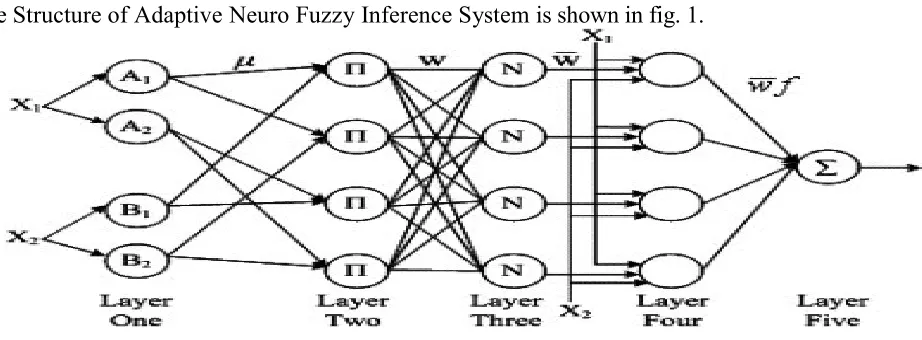
The Structure of Adaptive Neuro Fuzzy Inference System is shown in fig. 1.

Figure 1: Structure of Adaptive Neuro Fuzzy Inference System.

The Neuro Fuzzy models are gradually becoming established not only in the academia but also in the software applications. The tools for building Neuro Fuzzy models are based on combinations of algorithms from the fields of neural networks, pattern recognition and regression analysis.

1.4 Objectives

(3)

International Journal of Research (IJR)

 To collect the set of dataset program from running software with the appropriate runtime errors that is useful for the assessment.

 To formulate a theoretical analysis for the evaluation of the metrics those are used for assessment and develop model.

 To identify how availability and MTBF relates with the software reliability

 Calculate the metrics with the given dataset both analytically and programmatically.

 To train the neural network with some collected software reliability parameters (at design phase of SDLC) mapped to numerical data and are loaded into neural network at input layer.

 Assess and evaluate the performance of the trained network for software reliability at the design level with some numerically approximated values by using fuzzy membership function (sigmoid).

 The approximated Software Reliability is compared against the expected reliability approximation.

 The Neuro Fuzzy model was to adjust at the input layer has to minimize the difference between actual and expected values of reliability.

 Our proposed model performance compared against conventional FIS (Fuzzy Inference system) models based on evaluation and validation metrics to prove that our proposed model is the promising one than the others.

2. Proposed Approach for Reliability Assessment

2.1 Introduction

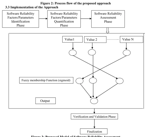
Figure below shows the proposed model of the research analysis, where the parameters concerned with the reliability assessment were given as the inputs for network. Weights are been added at the consequent layer ad using the predefined rules a decision is obtained at the validation. Based upon the outcome of validation the assessment will be finalized. A generalized block diagram is shown in the below figure, the parameters used were discussed in the next chapter. In this research work a Neuro Fuzzy interference model is designed for the assessment of reliability of a software growth model, the algorithm mainly focuses on MTBF and Availability which is analyzed and calculated theoretically and practically.

Fuzzy rules employed for the proposed model

 If MTBF (Mean time Between Failure) >0.8 & availability >0.8 then reliability is very

high

 If 0.7<MTBF <0.8 & 0.7< availability <0.8 then reliability is high  If 0.6<MTBF <0.7 & 0.6<availability <0.7 then reliability is moderate  If 0.5<MTBF <0.6 & 0.5< availability <0.6 then reliability is low  If 0.4<MTBF <0.3 & 0.4<availability <0.3 then reliability is very low

2.1.1 Identification Phase At this stage the objectives are 1. To identify the reliability factors.

(4)

International Journal of Research (IJR)

2.1.2 Quantification Phase At this stage the objectives are

1. To identify the reliability factors with availability and MTBF and to quantify them. 2. To evaluate a mathematical analysis for the relationship.

2.1.3 Measurement

At this stage the objectives are

1. To assess the metrics for the estimation of reliability 2. To validate the metrics

2.1.4 Verification and Validation Phase At this stage the objectives are

1. To estimate reliability 2. To validate the reliability

2.1.5 Finalization Phase At this stage the objectives are

1. To incorporate the changes and suggestions 2. To finalize the metrics for evaluation

2.1.6 Review & Revisions

(5)

International Journal of Research (IJR)

Figure 2: Process flow of the proposed approach 3.3 Implementation of the Approach

……..

………..

Figure 3: Proposed Model of Software Reliability Assessment

Mathematical approximation of proposal model metrics

For approximating the values of the proposed model metrics, a quantitative approach is adopted for calculating the appropriate results. The formula that has been used to calculate approximated values is defined as:

Formula: Ca ( xi ) = C (a) - h X f(a), based on Euler‟s theorem Where, C (a) = Set of Measured values.

Software Reliability Factors/Parameters

Identification Phase

Software Reliability Factors/Parameters

Quantification Phase

Software Reliability Assessment

Phase

Value1 Value 2 Value N

Fuzzy membership Function (sigmoid)

Output

Verification and Validation Phase

(6)

International Journal of Research (IJR)

„h‟ can be derived by, x1 + x0 n h

Where, n= no. of values in the dataset. x0 = 0 and x1 = 1 (since the probability ranges from 0 to 1). Here „x‟ is MTBF. f(a) can be function, denoted as

f(a)=MTBF/(1+MTBF)

Ca (xi ) is the set of values to be approximated.

Procedure for ‘h’ Calculation:

Let us take, x0 = 0 and x1 = 1 then, 1= 0 + 17 * h h= 1/17 = 0.058

Iterations: Perform at least 5 to 10 iterations to arrive at good approximated software reliability value. At every iteration, to calculate % of Reliability, use the following formula

% of Reliability = (Average of Approximated values)/ (Average of Measured values) * 100 At final iteration, if we got 99.99% or 99.8% or 99.7%, then we can say that it is good approximation.

4.2 Empirical Validation

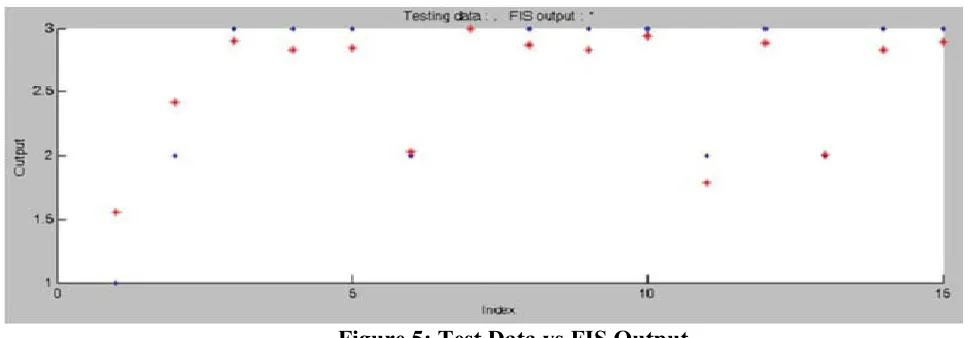
Below figure the practical implementation of the FIS model in MATLAB software [151] tool using FIS. The NF system is trained using a hybrid learning algorithm using both least squares method and back propagation algorithm. In the forward pass the consequent parameters are identified using least squares and in the backward pass the premise parameters are identified using back propagation [12]. The trained NF system is then tested for the fifteen inputs

(7)

International Journal of Research (IJR)

Figure 5: Test Data vs FIS Output

And it shows 0.1571, 0.2140 as NRMSE, RMSE (equations can be found in parameters to be evaluated section) values respectively. The plot of the expected and the output of the NF system for the different inputs are shown.

4.3 Dataset

To validate our model, we had taken 17 programs of Glace EMR Medical Billing Software (on which I had worked previously as a Software Engineer at L Cube Innovative Solutions Pvt. Ltd.,) and find out the MTTF (Mean Time to Failure), MTTR (Mean Time to Repair) and MTBR (Mean Time Between Repair) and Software Reliability Approximated value based on the program execution observations. We input these 3 values as input to input layer of Neural Network and apply sigmoid fuzzy membership function at the hidden layer of neural network and try to find out the software reliability approximated value. The previous values assessed using conventional traditional software reliability growth models and our Neuro Fuzzy systems based model are compared and we found to be our model is the promising one.

Software reliability is measured in terms of mean time between failures(MTBF).MTBF consists of mean time to failure (MTTF) and mean time to repair(MTTR). MTTF is the difference of time between two consecutive

failures and MTTR is the time required to fix the failure.

Let us take Software Reliability for good software is a number between 0 and 1. Reliability increases when errors or bugs from the program are removed or minimized. For example, if MTBF = 1000 hours for average software, then the software should work for 1000 hours for continuous operations. The dataset contains failure observations of 17 programs in Glace EMR Billing Software, in time series (i, Xi) and is used to predict the performance of the proposed model. Where, i = Program serial number.

(8)

International Journal of Research (IJR)

Table 1: Software Reliability data project information Software

Code

Type of Application Size(LOC) No. of Failures

GE01 Patient Registration 22,300 235

GE06 Service Entry 4,870 5

GE10 Reports 10,890 117

GE11 Reports 28,740 333

GE12 Reports 36,350 375

GE13 Online Patient Insurance Verification

61,800 821

GE14 Online Patient Insurance

Verification 34,700 354

39,800 383

43,200 412

GE17 Online Patient Insurance

(9)

International Journal of Research (IJR)

4.4 Parameters used for Validation

Reliability can be defined as the probability of failure free operation under stated conditions for specific period of time [70].Assessment of reliability performance for a component are usually defined for the expected input profile in actual operational use.

The commonly used metric for assessment are, Mean time to time failure (MTTF), mean time between failures (MTBF) and robustness [71].In [72] storey has given the definition as a function of time R(t) at a constant failure rate of λ

𝑅 𝑡 = 𝑒−𝜆𝑡

Where λ is the probability that there is no failure before time t Then the MTTF can be given as

𝑀𝑇𝑇𝐹 =1

𝜆

And

𝑀𝑇𝐵𝐹 = 𝑀𝑇𝑇𝐹 + 𝑀𝑇𝑇𝑅

Where MTTR is the mean time of recovery defined as the average time a component takes to recover from a failure. The measures MTBF, MTTF and MTTR are usually considered to apply in the case of a system operating continuously; however for a system operating on demand as is the case here, equivalent definitions apply where time is treated in discrete units [7].

Reliability can be defined as the probability of failure free operation under stated conditions for specific period of time [70].Assessment of reliability performance for a component are usually defined for the expected input profile in actual operational use.

Software reliability is measured in terms of mean time between failures(MTBF).MTBF consists of mean time to failure (MTTF) and mean time to repair(MTTR). MTTF is the difference of time between two consecutive failures and MTTR is the time required to fix the failure.

Let us take Software Reliability for good software is a number between 0 and 1. Reliability increases when errors or bugs from the program are removed or minimized.

For example, if MTBF = 1000 hours for average software, then the software should work for 1000 hours for continuous operations.

The dataset contains failure observations of 17 programs in GlaceEMR Billing Software, in time series (i, Xi) and is used to predict the performance of the proposed model.

Where, i = Program serial number.

Xi = No. of Failures of Program after ith modification has been done.

MTTF = Average time between 2 observed failures. i.e., average time it takes for a system to fail

For stable software system, MTTF = 1/ROCOF.

Where, ROCOF = Rate of fault occurrence corresponds to failure intensity.

Example, if ROCOF = 0.04 means 4 failures for each 100 operational time units of operation. MTBF = Average time between consecutive software system failures =MTTF+MTTR MTTR = Average time taken to repair the system after the occurrence of failure. Software Reliability

1. It is one of the metric used to measure the quality factor of the software system. 2. The software system facing rare failures is more reliable than the system facing more often failures. A System without faults is considered to be High Reliable. An Incorrect System is also reliable if the rate of failure is at acceptable level.

(10)

International Journal of Research (IJR)

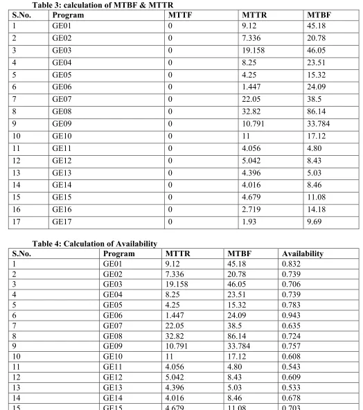
Availability = MTBF/(MTBF+MTTR)

4.6 Experimental Results

Table 2: Production Time Analysis for the Program Dataset S.N o. Program # Total Produc tion time(H rs.) Uptime at x1(Hrs.) Uptime at x2(Hrs.) Downtim e at x1(Hrs.) Downtime at x2(Hrs.) No. of breakdowns at x1(Hrs.) No. of breakdow ns at x2(Hrs.)

1 GE01 256 216 202 40 54 3 11

2 GE02 324 260 203 64 121 9 16

3 GE03 236 168 154 68 82 2 19

4 GE04 600 450 435 150 165 16 23

5 GE05 371 300 265 71 106 13 35

6 GE06 447 430 410 17 37 15 21

7 GE07 865 560 525 305 340 10 25

8 GE08 843 615 575 228 268 4 31

9 GE09 943 720 706 223 237 17 28

10 GE10 135 85 78 50 57 4 6

11 GE11 242 130 132 112 110 36 22

12 GE12 369 240 206 129 163 24 30

13 GE13 122 68 64 54 58 23 9

14 GE14 107 72 74 35 33 6 15

15 GE15 371 265 253 106 118 18 34

16 GE16 453 370 398 83 55 21 37

17 GE17 325 285 256 40 69 27 29

Calculations

Total Production time= Uptime+ down time MTBF= Total uptime (total time- total downtime) Number of Breakdowns

(Or) MTTF+ MTTR Where,

MTTF= Mean Time to Failure (in hours/minutes/seconds). MTTR= Mean Time to Repair (in hours/minutes/seconds).

MTBF= Mean Time between Failures (in hours/minutes/seconds). MTTR= Total downtime

Number of breakdowns

MTTF= (Failure at obs.1+ Failure at obs.2+…+ Failure at obs.N) Number of software programs under test

(11)

International Journal of Research (IJR)

(MTBF+ MTTR) Table 3: calculation of MTBF & MTTR

S.No. Program MTTF MTTR MTBF

1 GE01 0 9.12 45.18

2 GE02 0 7.336 20.78

3 GE03 0 19.158 46.05

4 GE04 0 8.25 23.51

5 GE05 0 4.25 15.32

6 GE06 0 1.447 24.09

7 GE07 0 22.05 38.5

8 GE08 0 32.82 86.14

9 GE09 0 10.791 33.784

10 GE10 0 11 17.12

11 GE11 0 4.056 4.80

12 GE12 0 5.042 8.43

13 GE13 0 4.396 5.03

14 GE14 0 4.016 8.46

15 GE15 0 4.679 11.08

16 GE16 0 2.719 14.18

17 GE17 0 1.93 9.69

Table 4: Calculation of Availability

S.No. Program MTTR MTBF Availability

1 GE01 9.12 45.18 0.832

2 GE02 7.336 20.78 0.739

3 GE03 19.158 46.05 0.706

4 GE04 8.25 23.51 0.739

5 GE05 4.25 15.32 0.783

6 GE06 1.447 24.09 0.943

7 GE07 22.05 38.5 0.635

8 GE08 32.82 86.14 0.724

9 GE09 10.791 33.784 0.757

10 GE10 11 17.12 0.608

11 GE11 4.056 4.80 0.543

12 GE12 5.042 8.43 0.609

13 GE13 4.396 5.03 0.533

14 GE14 4.016 8.46 0.678

(12)

International Journal of Research (IJR)

16 GE16 2.719 14.18 0.839

17 GE17 1.93 9.69 0.833

Figure 6: Analysis of Availability Ration w.r.t. Number of Programs

(13)

International Journal of Research (IJR)

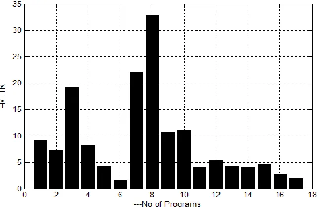
Figure 8: Analysis of MTBF ration w.r.t. number of Programs

Theoretical Validation

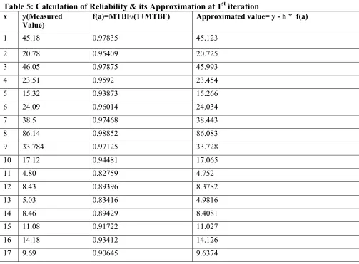
From the above section 3.11 a theoretical valuation can be done with the formula mentioned in the context. For example at the 1st Iteration

Table 5: Calculation of Reliability & its Approximation at 1st iteration x y(Measured

Value)

f(a)=MTBF/(1+MTBF) Approximated value= y - h * f(a)

1 45.18 0.97835 45.123

2 20.78 0.95409 20.725

3 46.05 0.97875 45.993

4 23.51 0.9592 23.454

5 15.32 0.93873 15.266

6 24.09 0.96014 24.034

7 38.5 0.97468 38.443

8 86.14 0.98852 86.083

9 33.784 0.97125 33.728

10 17.12 0.94481 17.065

11 4.80 0.82759 4.752

12 8.43 0.89396 8.3782

13 5.03 0.83416 4.9816

14 8.46 0.89429 8.4081

15 11.08 0.91722 11.027

16 14.18 0.93412 14.126

(14)

International Journal of Research (IJR)

At 2nd iteration

Table 6: Calculation of Reliability & its Approximation at 2nd iteration

x y(Measured Value) f(a)=MTBF/(1+MTBF) Approximated value= y - h * f(a)

1 45.123 0.97835 45.066

2 20.725 0.95409 20.67

3 45.993 0.97875 45.936

4 23.454 0.9592 23.398

5 15.266 0.93873 15.212

6 24.034 0.96014 23.978

7 38.443 0.97468 38.386

8 86.083 0.98852 86.026

9 33.728 0.97125 33.672

10 17.065 0.94481 17.01

11 4.752 0.82759 4.704

12 8.3782 0.89396 8.3264

13 4.9816 0.83416 4.9332

14 8.4081 0.89429 8.3562

15 11.027 0.91722 10.974

16 14.126 0.93412 14.072

17 9.6374 0.90645 9.5848

At 3rd Iteration

Table 7: Calculation of Reliability & its Approximation at 3rd iteration

x y(Measured Value)

f(a)=MTBF/(1+MTBF) Approximated value= y - h * f(a)

1 45.066 0.97835 45.009

2 20.67 0.95409 20.615

3 45.936 0.97875 45.879

4 23.398 0.9592 23.342

5 15.212 0.93873 15.158

6 23.978 0.96014 23.922

7 38.386 0.97468 38.329

8 86.026 0.98852 85.969

9 33.672 0.97125 33.616

10 17.01 0.94481 16.955

11 4.704 0.82759 4.656

12 8.3264 0.89396 8.2746

13 4.9332 0.83416 4.8848

14 8.3562 0.89429 8.3043

15 10.974 0.91722 10.921

16 14.072 0.93412 14.018

(15)

International Journal of Research (IJR)

At 4th Iteration

Table 8: Calculation of Reliability & its Approximation at 4th Iteration

1 45.009 0.97835 44.952

2 20.615 0.95409 20.56

3 45.879 0.97875 45.822

4 23.342 0.9592 23.286

5 15.158 0.93873 15.104

6 23.922 0.96014 23.866

7 38.329 0.97468 38.272

8 85.969 0.98852 85.912

9 33.616 0.97125 33.56

10 16.955 0.94481 16.9

11 4.656 0.82759 4.608

12 8.2746 0.89396 8.2228

13 4.8848 0.83416 4.8364

14 8.3043 0.89429 8.2524

15 10.921 0.91722 10.868

16 14.018 0.93412 13.964

17 9.5322 0.90645 9.4796

At 5th Iteration

Table 9: Calculation of Reliability & its Approximation at 5th iteration

1 44.952 0.97835 44.895

2 20.56 0.95409 20.505

3 45.822 0.97875 45.765

4 23.286 0.9592 23.23

5 15.104 0.93873 15.05

6 23.866 0.96014 23.81

7 38.272 0.97468 38.215

8 85.912 0.98852 85.855

9 33.56 0.97125 33.504

10 16.9 0.94481 16.845

11 4.608 0.82759 4.56

12 8.2228 0.89396 8.171

13 4.8364 0.83416 4.788

14 8.2524 0.89429 8.2005

15 10.868 0.91722 10.815

16 13.964 0.93412 13.91

(16)

International Journal of Research (IJR)

% Reliability= (Average of Approximated vales/ Average of observed Values) x 100

In 5th iteration, we got 99.70%, so we will stop iteration process because we got good approximated % of reliability.

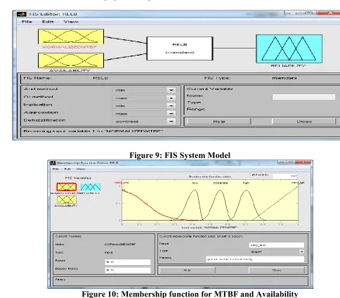
Practical Validation

The experiment was conducted with 17 programs of Glace EMR Medical Billing the analysis was done using FIS (fuzzy interference system) and the proposed Neuro Fuzzy model. The model structure and error tolerance graphs are depicted below.

Figure 9: FIS System Model

Figure 10: Membership function for MTBF and Availability

(17)

International Journal of Research (IJR)

Figure 11: Neuro Fuzzy Inference Model

(18)

International Journal of Research (IJR)

Figure 13: Error Tolerance

Figure 14: Performance Analysis

Comparison of proposed approach with Conventional Fuzzy system

(19)

International Journal of Research (IJR)

environment (See Appendix-A). From the above the performance assessment for which an improvement of 11% is achieved with the current proposal.

MSE= ((Theoretical validation- practical Validation)/total no of readings)2

=

Average error = ((Theoretical validation- practical Validation)/total no of readings)=0.247;

Figure 15: Practical Validation of the Reliability percentage obtained using MATLAB

Table 10: Performance comparison between FIS & ANFIS of SR estimation

Method MSE AE

FIS 0.799 0.894

ANFIS 0.061 0.247

5.6 Future Work and Suggestions

Software reliability can be predicted using hybrid intelligent system. In addition to neural

network model genetic programming can be applied further. Novel recurrent architectures for Genetic Programming (GP) and Group Method

(20)

International Journal of Research (IJR)

of Data Handling (GMDH) to predict software reliability can be proposed. Software reliability can be predicted using hybrid intelligent system. In addition to neural network model genetic programming can be applied further. Novel recurrent architectures for Genetic Programming (GP) and Group Method of Data Handling (GMDH) to predict software reliability can be proposed. We can explore other soft computing techniques and other different data set.

5.7 Limitations

Every research suffers from some limitations. No Researcher can perform a full fledged work. Here in our research, Availability and MTBF are taken as factors for identifying the Software Reliability and we perform our research study. High Availability increases the reliability of the software. The study suffers from the following limitations:

 The model can be used to maximize and measure the availability, MTBF and maximize and assess software reliability based on Neuro Fuzzy systems approach.

 The model was validated with only a small dataset(17 programs of GlaceEMR software).

 The research concentrated on reliability factors like availability, MTBF and uptime, downtime, number of breakdowns only.

5.8 Conclusion

From the research we found that Neuro Fuzzy model performs better in terms of less error in prediction as compared to existing analytical models and hence it is a better alternative to do software reliability test. As the weights are randomly initialized, thus the model gives different results for the same datasets and thus the performance of the model varies. The usefulness of a Neuro Fuzzy model is dependent on the nature of dataset up to a greater extent.

The preliminary computational results in the MATLAB environment seem quite promising and give insight into the generalization capability of these models. The results of the fuzzy logic and neural networks models were very promising. The error difference between the actual and estimated response was small. This finding gives a good indication of prediction capabilities of the developed fuzzy model and neural networks for assessing the software reliability. After evaluation of our proposed model, we can say that we proposed improved Neuro Fuzzy systems based approach for software reliability assessment as compared to the existing conventional fuzzy logic based software reliability growth assessment and evaluation models based on the experimental results.

References

[1] Hoyer, R. W. and Hoyer, B. B. Y., "What is quality?" Quality Progress, no. 7, pp. 52-62, 2001.

[2] Crosby P.B,” Quality is Free the Art of Making Quality Certain NY, McGraw –Hill-1979

[3] Deming & Edwards W,”Out of Crisis”, MIT Press-1986

[4] Feigenbaum A. V, "Total Quality Control”, McGraw – Hill-1983

[5] IEEE Std 610.12 (1990). IEEE Standard Glossary of Software Engineering Terminology, NY.

(21)

International Journal of Research (IJR)

[7] McCall J.A, Richards P.K & Walters G.F,” Factors in Software Quality”, Nat'1 Tech Information Services, - Vol 1-2, 1977

[8] AIAA/ANSI “Recommended Practice for Software Reliability, the American Institute of Aeronautics and Astronautics”, Washington DC, Aerospace Center, R-013, 1992,-ISBN 1-56347-024-1.

[9] Michael R. Lyu,” Handbook of software Reliability Engineering “, IEEE

[10] Wasserman, Gary . Reliability verification, Testing and analysis in engineering design. Marcel Dekker incorporated, Newyork, USA, pp2-10, 2002

[11] Schneidewind, N. F., 2001, „Modeling the fault correction processes, Proceedings of the 12th International Symposium on Software Reliability Engineering, pp. 185-190.

[12] Myrtveit, I., Stensrud, E. and Shepperd, M., 2005, „Reliability and validity in comparative studies of software prediction models‟, IEEE Transactions on Software Engineering, vol. 31, no. 5, pp. 380-391.

[13] Falcone, G. Hierachy-aware Software Metrics in Component Composition Hierarchies. PhD thesis, University of Mannheim.-2010

[14] Bass, L., Clements, P., and Kazman, R. “Software Architecture in Practice” , Second Edition. Addison-Wesley, Reading, MA, USA-2003

[15] Jain, R. The Art of Computer Systems Performance Analysis: Techniques for Experimental Design, Measurement, Simulation, and Modeling. Wiley.-1991

[16] Smith, C. U. and Williams, L. G. (2000). Software performance anti patterns. In Workshop on Software and Performance, pages 127-136.

[17] Immonen, A. and Niemel•a, E.,” Survey of reliability and availability prediction methods from the viewpoint of software architecture. Software and System Modeling-7(1):49{65)-2008

[18] AIAA/ANSI “Recommended Practice for Software Reliability, The American Institute of Aeronautics and Astronautics”, Washington DC, Aerospace Center, R-013, 1992,-ISBN 1-56347-024-1.

[19] Rosenberg Linda, Hammer Ted & Shaw Jack, “Software Matrices and Reliability”, ISSRE, 1998.

[20] N. E. Fenton and M. Neil. A critique of software defect prediction models. IEEE Transactions on Software Engineering, 25(5):675–689, 1999.

[21] N. E. Fenton and N. Ohlsson. Quantitative analysis of faults and failures in a complex software system. IEEE Transactions on Software Engineering, 26(8):797–814, 2000

[22] Wood Alan. Software Reliability Growth Models, Tandem Technical Report- Vol 19.1-part number 130056, 1996.

[23] Lyu M.R, Handbook of Software Reliability Engineering, IEEE Computer Society Press, 1996.

(22)

International Journal of Research (IJR)

[25] L. Tian and A. Noore, “Software Reliability Prediction Using Recurrent Neural Network with Bayesian Regularization,” International Journal of Neural Systems, vol. 14, no. 3, pp. 165–174, June 2004

[26] P.Werbos, “Generalization of Back propagation with Application to Recurrent Gas Market Model,” Neural Network, vol. 1, pp. 339–356, 1988.

[27] R. Shadmehr and D. Z. DSArgenio, “A Comparison of a Neural Network Based Estimator and Two Statistical Estimators in a Sparse and Noisy Data Environment,” in IJCNN, vol. 1, Washington D.C, pp. 289–292, June 1990. [28] N. Karunanithi, Y. Malaiya, and D. Whitley, “Prediction of Software Reliability Using Neural

Networks,” in Proceedings IEEE International Symposium on Software Reliability Engineering. Austin, TX: IEEE, pp. 124–130, May 1991.

[29] T. M. Khoshgoftaar, A. S. Pandya and H. More, “A Neural Network Approach For Predicting Software Development Faults.” Research Triangle Park, NC: Proceedings of Third International Symposium on Software Reliability Engineering, pp. 83–89, October 1992.

[30] Y. Singh and P. Kumar, “Prediction of Software Reliability Using Feed Forward Neural Networks,” in Computational Intelligence and Software Engineering (CiSE), I. Conference, Ed.

IEEE, pp. 1–5, 2010.

Appendix- A

MATLAB Program for Practical Validation clear

% MTBF input

aa= VECTOR OF MTBF VALUES; af=aa./mean(aa);

% Availability Input

b= VECTOR OF AVAILABILITY VALUES; % Read the FIS structure named as RELB F=readfis('RELB.fis');

% Evalate the input with the given fuzzy structre ff=evalfis([aa./max(aa)+.7,b+.7]',F)

% this section is regarding ANFIS

% train the data for it give MTBF and Availability as inputs trnData = [af , b];

numMFs = 7; mfType = 'dsigmf'; epoch_n = 100;

% generate a new anfis with this training data in_fis = genfis1(trnData,numMFs,mfType); out_fis = anfis(trnData,in_fis,60);

ff' mean(ff)

(23)

International Journal of Research (IJR)

mean(oo)

Mr. Bonthu Kotaiah obtained his Bachelor's degree in Computer Applications from Nagarjuna University in 2001 and M.C.A from Nagarjuna University in 2008. During the period from September, 2001 to 2011, he has been involved in various aspects of Information Technology - an engineer(L-Cube Innovative Solutions), a Corporate Trainer (SyncSoft & Datapro(Vijayawada), COSS(Hyd.)), a Computer Programmer(Acharya Nagarjuna University). Currently he wishes to conduct research in the area of Software Engineering and Data Mining and Artifiicial Neural Networks, Fuzzy Logic & Genetic Alogorithms. His research interests include software Engineering, Neural networks. Presently, he is working as a Full-Time Research Scholar in Babasaheb Bhimrao Ambedkar University (A Central University) Lucknow, UP in the Department of Information Technology.