Wake Dynamics and Passive Flow Control of a Blunt Trailing Edge Profiled Body

(1)

Scholarship@Western

Electronic Thesis and Dissertation Repository

12-15-2010 12:00 AM

Wake Dynamics and Passive Flow Control of a Blunt Trailing Edge

Profiled Body

Lakshmana Sampat Doddipatla The University of Western Ontario

Supervisor Dr.Horia Hangan

The University of Western Ontario

Graduate Program in Civil and Environmental Engineering

A thesis submitted in partial fulfillment of the requirements for the degree in Doctor of Philosophy

Follow this and additional works at: https://ir.lib.uwo.ca/etd

Part of the Civil and Environmental Engineering Commons

Recommended Citation Recommended Citation

Doddipatla, Lakshmana Sampat, "Wake Dynamics and Passive Flow Control of a Blunt Trailing Edge Profiled Body" (2010). Electronic Thesis and Dissertation Repository. 71.

https://ir.lib.uwo.ca/etd/71

This Dissertation/Thesis is brought to you for free and open access by Scholarship@Western. It has been accepted for inclusion in Electronic Thesis and Dissertation Repository by an authorized administrator of

(2)

WAKE DYNAMICS AND PASSIVE FLOW CONTROL OF A BLUNT TRAILING

EDGE PROFILED BODY

(Thesis Format: Monograph)

by:

Lakshmana Sampat Doddipatla

Department of Civil and Environmental Engineering Faculty of Engineering Science

A thesis submitted in partial fulfillment of the requirements for the degree of

Doctor of Philosophy

The School of Graduate and Postdoctoral Studies The University of Western Ontario

London, Ontario, Canada

(3)

ii

THE UNIVERSITY OF WESTERN ONTARIO

THE SCHOOL OF GRADUATE AND POSTDOCTORAL STUDIES

CERTIFICATE OF EXAMINATION

Supervisor

______________________________ Dr. Horia Hangan

Examiners

______________________________ Dr. Craig Miller

______________________________ Dr. Diana Inculet

______________________________ Dr. Kamran Siddiqui

______________________________ Dr. SerhiyYarusevych

The thesis by

Lakshmana Sampat Doddipatla

Entitled

WAKE DYNAMICS AND PASSIVE FLOW CONTROL OF A BLUNT TRAILING

EDGE PROFILED BODY

is accepted in partial fulfillment of the requirements for the degree of

Doctor of Philosophy

(4)

iii

ABSTRACT

Wake flows behind two-dimensional bodies are dominated mainly by two types of

coherent structures, namely, the Karman Benard vortices and the streamwise vortices,

also referred to as rolls and ribs respectively. The three-dimensional wake instabilities

lead to distinct instability modes (mode-A, mode-B and mode-C or mode S) depending

on the flow Reynolds number and geometric shape. The present investigation explores

the mechanism by which the flow transitions take place to three-dimensionality in the

near wake of a profiled leading edge and blunt trailing edge body. Experiments

consisting of a combination of Planar Laser Induced Fluorescence visualizations and

Particle Image Velocimetry measurements are conducted for Reynolds numbers ranging

from 250 to 46000. The results indicate that three instability modes, denoted by

mode-A, mode-B and mode-C, appear in the wake transition to three-dimensionality, but their

order of appearance does not occur through the traditional route as observed in circular

cylinder flows. It is found that mode-C instability with a spanwise spacing varying

between 1.2 to 2.8D (D being the trailing edge thickness) dominates the near wake

development. This result is explored further with the aim to devise a simple passive

control method to mitigate vortex shedding for blunt trailing edge bodies.

The effect of a trailing edge spanwise sinusoidal perturbation (SSP) is investigated

for a range of Reynolds numbers (ReD) spanning the transition range from ReD = 550 up

to 46000. PIV measurements at different vertical and horizontal locations are performed

to study changes in the streamwise and spanwise vortices. The base drag and strength

of vortex shedding decrease with wavy trailing edge compared to the straight trailing

edge. Proper Orthogonal Decomposition (POD) of the obtained PIV data indicates that

the spanwise sinusoidal perturbation redistributes the relative energy, enhancing the

(5)

iv

KEYWORDS: Blunt Trailing-Edge-Profiled Body, Vortex Shedding, Wake Instabilities, Passive Flow Control, Drag Reduction, Particle Image Velocimetry (PIV), Planar Laser

(6)

v

CO-AUTHORSHIP

The dissertation uses monograph format specified by the school of graduate and

postdoctoral studies, The University of Western Ontario, London, Ontario, Canada.

Chapters 3 and 4 will be submitted for publication to Journal of Fluid Mechanics and

Experiments in Fluids, respectively. These papers are authored by Lakshmana Sampat

Doddipatla along with his supervisor, Horia Hangan, and co-authors Arash

Naghib-Lahouti, Vibhav Durgesh and Jonathan Naughton. Lakshmana Sampat Doddipatla is the

principal author, who conducted all the experiments and the data analysis, except for

PLIF and PIV water tunnel measurements for which the experimental data are shared

with Arash Naghib-Lahouti. The analysis however is carried independently. Vibhav

Durgesh helped with the experimental setup at the University of Wyoming Aeronautics

Laboratory under the supervision of Prof. Jonathan Naughton.

Chapter 3

Doddipatla, L.S., Lahouthi, A.N. & Hangan, H. Near wake topology of a profiled blunt

trailing edge body. To be submitted to J. Fluid Mech.

Chapter 4

Doddipatla, L.S., Hangan, H., Durgesh, V. & Naughton, J.W. Wake dynamics resulting

(7)

vi

(8)

vii

ACKNOWLEDGEMENT

It is with immense pleasure that I begin to write this section and I would like to

thank all those who have helped me to get to this stage. I sincerely thank my supervisor

Dr. Horia Hangan for his patience, guidance and direction throughout this work. I would

also like to thank Dr. Vibhav Durgesh and Dr. Jonathan Naughton at the University of

Wyoming for assisting me with wind tunnel experiments and providing helpful

discussions on the implementation of Proper Orthogonal Decomposition. I would also

like to thank Arash Naghib-Lahouti for assisting me with water tunnel measurements.

Thanks are due to Dr. Kamran Siddiqui for providing the PIV system for the water tunnel

experiments at The University of Western Ontario. Finally, I am grateful to Mr. Chris

Vandelaar for his assistance in the machine shop.

I want to express thanks to all of my colleagues at The Boundary Layer Wind Tunnel

Laboratory for their kindness and support. I am grateful to my friends Diwakar Natrajan,

Padmavathi Sagi and Bilal Bakht for making my stay in Canada a cherishable experience.

I express my deep gratitude to my parents, Dr. Vivekananda Prasad Doddipatla and

Giri Kumari Doddipatla, and my brother, Dr. Rama Sanand Doddipatla, for their

unwavering faith and continuous support during the long period of my education. I

would like to especially thank my wife, Kranthi, for her unlimited support,

(9)

viii

LIST OF FIGURES

Figure 1-1 Leonardo da Vinci: seated man and water studies

(http://www.royalcollection.org.uk) ... 2

Figure 1-2 Schematic of dominant near wake instabilities ... 3

Figure 1-3 Description of Mode-A, Mode-B and Mode-C structures in XY and XZ planes

(arrows indicate the vorticity direction) ... 5

Figure 2-1 Water tunnel experimental setup ... 16

Figure 2-2 Mean streamwise velocity at the centre line of the water tunnel at different

downstream locations (Sarathi 2009) ... 17

Figure 2-3 Variation of (a)mean streamwise velocity and (b) turbulence intensity at

different spanwise locations at X/h = 0.33 (Sarathi 2009) ... 18

Figure 2-4 Wind tunnel experimental setup ... 19

Figure 2-5 Variation of (a) mean streamwise velocity and (b) turbulence intensity profile

in the boundary layer at X/D = 0.4 before separation ... 20

Figure 2-6 A schematic showing the flat plate model used in the water tunnel, along

with the field of view for imaging planes and the coordinate axis ... 22

Figure 2-7 A schematic showing the flat plate model used in the wind tunnel, and the

major dimensions along with the field of view for PIV images and the

coordinate axis ... 24

Figure 2-8 Location of the pressure transducers ... 24

Figure 2-9 Details of the different trailing edges used in the wind tunnel measurements

... 25

Figure 2-10 Typical PIV system with (a) Integrated Cooling and Electronics (ICE) unit, (b)

laser head with sheet optics attached and (c) dual frame CCD camera and the

(13)

xii

Figure 2-11 The calibration sheet used for the PIV measurements in (a) water tunnel and

(b) wind tunnel ... 29

Figure 2-12 The velocity flow field data obtained after processing the PIV images ... 30

Figure 2-13 Flush mounted high speed transducers used in this investigation ... 31

Figure 2-14 Typical high speed pressure data acquisition setup ... 32

Figure 2-15 Calibration for (a) DP-15 transducer and (b) High speed pressure transducer ... 34

Figure 2-16 Acquisition timing for PIV and pressure records in wind tunnel measurements ... 35

Figure 2-17 Cumulative convergence of energy using snapshot POD in vertical plane for straight trailing edge at ReD = 24000. ... 38

Figure 2-18 Convergence of energy captured by (a) mode 1 and (b) mode 2 in XY plane, (c) mode 1 and (d) mode 2 in XZ plane (Y/D = -0.5), and (e) mode 1 and (f) mode 2 in XZ plane (Y/D = -0.5) at ReD = 24000. Energy is calculated using 10, 50, 100, 200, 300, 400, 500, 600, 700, 800, 900 and 1000 PIV images. ... 40

Figure 2-19. Comparison of streamwise turbulence intensity along the centre line calculated using standard deviation of the PIV data and reconstructed using different number of POD modes at (a) ReD = 550, (b) ReD = 1050,(c) ReD = 1550, (d) ReD = 2300, (e) ReD = 24000 and (f) ReD = 46000 ... 41

Figure 2-20. % error in predicting centre line streamwise turbulence intensity by combining different number of POD modes for ReD = 550, 1050, 1500, 2300, 24000 and 46000 ... 42

Figure 2-21 Correlation of phase angles determined from the POD coefficients and pressure signal in XY plane ... 44

(14)

xiii

Figure 2-23 Phase averaged streakline plots obtained by calculating the phase from the

(a) pressure signal, (b) POD coefficients and (c) conditional averaging

approach. ... 46

Figure 3-1. Comparison of Strouhal number as a function of Reynolds number with

Petrusma and Gai (1996) ... 48

Figure 3-2. Comparison of Roshko number as a function of Reynolds number with Bull et

al. (1995) ... 50

Figure 3-3. Comparison of Roshko number as a function of Reynolds number with Ryan

et al. (2005) ... 51

Figure 3-4. Instantaneous (a) streamwise velocity, (b) transverse velocity and (c) z

vorticity for Reynolds numbers of (I) ReD = 550, (II) ReD = 1050, (III) ReD = 1550

and (IV) ReD = 2300 ... 53

Figure 3-5. (a) Streamwise and (b) transverse velocity components for the first nine POD

modes in XY plane at ReD= 550 ... 54

Figure 3-6. Relative energy captured by first ten POD modes in XY plan at ReD = 550 .... 56

Figure 3-7. Phase averaged time varying coefficient in XY plane at ReD = 550 ... 56

Figure 3-8. Phase portraits of time varying coefficient in XY plane at ReD = 550. The solid

line indicates the phase averaged relation between these POD modes. ... 57

Figure 3-9. (a) PLIF Visualization (b) streakline plot along with vorticity contours of the

first two POD modes in XY plane at ReD = 550 ... 59

Figure 3-10. Streamwise and transverse velocity components for the first five POD

modes in XY plane at (a) ReD = 1050, (b) ReD = 1550 and ReD = 2300... 60

Figure 3-11. (a) Relative energy captured by first ten POD modes in XY plan at ReD =

1050, 1550 and 2300. Phase averaged time varying coefficient in XY plane at

(b) ReD = 1050, (c) ReD = 1550 and (a) ReD = 2300 ... 61

Figure 3-12. PLIF visualization and the streakline plots along with vorticity contours by

combining first two POD modes of in XY plane for (a) ReD = 1050, (b) ReD =

(15)

xiv

Figure 3-13. Streamwise spacing of spanwise vortices as a function of Reynolds number

... 63

Figure 3-14. PLIF visualization at ReD = 250 in XZ plane (Y/D = -0.5) (a) parallel vortex shedding (b) vortex dislocation, (c) visualization of the vortex dislocation (Williamson 1992), and (d) schematic representation of vortex dislocation (Williamson 1992). ... 64

Figure 3-15. PLIF visualization at ReD = 300 in XZ plane (Y/D = -0.5) (a) parallel vortex shedding (b) vortex dislocation and (c) three-dimensional features ... 65

Figure 3-16. PLIF visualization at ReD = 350 in XZ plane (Y/D = -0.5) (a) parallel vortex shedding (b) vortex dislocation and (c) mushroom structures ... 66

Figure 3-17. PLIF Visualization in XZ plane (Y/D = -0.5) at ReD = 400 ... 67

Figure 3-18. PLIF Visualization in YZ plane (X/D = 3) at ReD = 400 ... 68

Figure 3-19. PLIF Visualization in XZ plane (Y/D = -0.5) at ReD = 550 ... 69

Figure 3-20. PLIF Visualization in YZ plane (X/D = 3) showing the dislocations caused due to streamwise vortices in spanwise vortices at ReD = 550 ... 70

Figure 3-21. Schematics of the primary and secondary vortices of (a) mode-A (b) mode-B topologies. Vorticity sign is marked by arrows. ... 71

Figure 3-22. PLIF Visualization in XZ plane (Y/D = -0.5) at ReD = 550 for (a) straight trailing edge and (b) sinusoidal trailing edge ... 73

Figure 3-23. Mean streamwise velocity contours in XZ plane (Y/D = -0.5) at ReD = 550 for (a) straight trailing edge and (b) sinusoidal trailing edge ... 74

Figure 3-24. Comparison of mean centre line velocity for straight trailing edge and sinusoidal trailing edge ... 74

Figure 3-25. Instantaneous (a) streamwise velocity, (b) spanwise velocity and (c) y vorticity for Reynolds numbers of (I) ReD = 550, (II) ReD = 1050, (III) ReD = 1550 and (IV) ReD = 2300 ... 76

(16)

xv

Figure 3-27. y vorticity contours in XZ plane (Y/D = -0.5) at ReD = 400 by combing POD

modes (a) 1 to 4, (b) 5 to 8, and (c) 9 and 10. ... 79

Figure 3-28. Schematic of the primary and secondary structures ... 80

Figure 3-29. Streamwise velocity contour in XZ plane (Y/D = -0.5) at ReD = 400 by combining POD modes 1 to 32 ... 80

Figure 3-30. Schematic of mode-A in (a) XY plane and (b) XZ plane ... 80

Figure 3-31. y vorticity contours in XZ plane (Y/D = -0.5) at ReD = 550 by combing POD modes (a) 1 to 4, (b) 5 and 6, (c) 7 and 8, and (d) 9 to 12 ... 82

Figure 3-32 Relative energy captured by first 15 POD modes in XZ planes (Y/D = -0.5 and Y/D = 0) at ReD = 550 ... 83

Figure 3-33 y vorticity contours in XZ plane (Y/D = 0) at ReD = 550 by combining POD modes 1 to 10 ... 83

Figure 3-34. y vorticity contour in XZ plane (Y/D = -0.5) at ReD = 550 by combing POD modes (a) 1 and 2, (b) 3 and 4, (c) 5 and 6, (d) 7 and 9, (e) 9 to 12. (f) Streamwise velocity contour by combining POD modes 1 to 32 ... 85

Figure 3-35. (a) y vorticity contour in XZ plane (Y/D = 0) at ReD = 550 by combing POD modes 1 to 10 and (b) streamwise velocity contour by combining POD modes 1 to 32 ... 86

Figure 3-36. PLIF visualization in XZ plane (Y/D = -0.5) at ReD = 1050 ... 87

Figure 3-39 Relative energy captured by first 15 POD modes in XZ planes (Y/D = -0.5) at ReD = 1050, 1550 and 2300 ... 89

(17)

xvi

Figure 3-41. (a) y vorticity contour in XZ plane (Y/D = -0.5) at ReD = 1550 by combing

POD modes (a) 1 and 2, (b) 3 and 4, (c) 5 and 6, (d) 7 and 8. (e) Streamwise

velocity contour by combining POD modes 1 to 32 ... 91

Figure 3-42. (a) y vorticity contour in XZ plane (Y/D = -0.5) at ReD = 2300 by combing

POD modes (a) 1 and 2, (b) 3 and 4, (c) 5 and 6, (d) 7 and 8. (f) Streamwise

velocity contour by combining POD modes 1 to 32 ... 92

modes in XY plane for the base case at ReD = 24000 ... 94

modes in XY plane for the base case at ReD = 46000 ... 94

Figure 3-45. (a) Relative energy captured by first ten POD modes in XY plane at ReD =

24000 and 46000. Phase averaged time varying coefficient in XY plane at (b)

ReD = 24000 and (c) ReD = 46000... 95

Figure 3-46. Streakline plots along with vorticity contours by combining first two POD

modes of in XY plane for (a) ReD = 24000 and (b) ReD = 46000 ... 96

Figure 3-47. Relative energy captured by first 15 POD modes in XZ at (a) Y/D = -0.5 and

(b) Y/D = 0 plane for ReD = 24000 and ReD = 46000 ... 97

Figure 3-48. Streamwise and transverse velocity components for the first ten POD

modes in XZ plane for the base case at ReD = 24000 ... 98

Figure 3-49. Streamwise and transverse velocity components for the first ten POD

modes in XZ plane for the base case at ReD = 46000 ... 99

Figure 3-50 Sreamwise velocity contours in XZ plane (Y/D = -0.5) at ReD = 24000 by

combining POD modes 1 to 32 at different instances in flow ... 100

Figure 3-51 Streamwise velocity contours in XZ plane (Y/D = -0.5) at ReD = 46000 by

combining POD modes 1 to 32 at different instances in flow ... 101

Figure 4-1. Wavy square cylinder flow regime (Darekar and Sherwin 2001) ... 105

Figure 4-2. Comparison of base pressure coefficient for (a) straight and SSP(z/D = 2.4

(18)

xvii

Figure 4-3. Comparison of the mean streamwise velocity profiles at various downstream

locations for ReD = 550 ... 110

Figure 4-4. Comparison of base drag coefficient for straight and SSP (z/D = 2.4) trailing

edges at ReD = 550, 1550 and 2300. ... 111

Figure 4-5. Streamwise mean velocity contour at Y/D = -0.5 for SSP (z/D = 2.4) trailing

edge at ReD = 24000 ... 112

Figure 4-6. Comparison of mean streamwise centre line velocity for straight and SSP

(z/D = 2.4) trailing edges at (a) ReD = 550, (b) ReD =1550, (c) ReD = 2300, (d)

ReD =24000 and (e) ReD = 46000 ... 113

Figure 4-7. Comparing streamwise turbulence intensity profiles at mid-plane for base

case and SSP (z/D = 2.4) control case at (a) ReD = 550, (b) ReD =1550, (c) ReD =

2300, (d) ReD =24000 and (e) ReD = 46000. (f) Comparing formation lengths for

base case and SSP (z/D = 2.4) control case at different Reynolds numbers 115

Figure 4-8. Schematic of the PIV measurement window in the horizontal (XZ) plane .. 116

Figure 4-9. Streakline plots at different phases of vortex shedding in XY for base case

and SSP (z/D = 2.4) control case at ReD = 24000 ... 117

Figure 4-10. Comparison of peak vorticity variation for straight and SSP (z/D = 2.4)

trailing edges at different Reynolds numbers ... 118

Figure 4-11. Comparison of power spectral density for straight and SSP (z/D = 2.4)

trailing edges for (a) base case (b) MAX (c) MED (d) MIN at (I) ReD = 550, (II)

ReD = 1550, (III) ReD = 2300, (IV) ReD = 24000 and (V) ReD = 46000 ... 119

modes in XY plane for SSP (z/D = 2.4) control case at (a) MAX and (b) MIN

locations for ReD = 24000 ... 122

Figure 4-13. Phase averaged time varying coefficient in XY plane for (a) SSP 2.4: MAX

(19)

xviii

Figure 4-14. Streamwise and transverse velocity components for the first nine POD

modes in XY plane for SSP (z/D = 2.4) control case at MAX location for ReD =

550 ... 123

Figure 4-15. Streamwise and transverse velocity components for the first nine POD

modes in XY plane for SSP (z/D = 2.4) control case at MIN location for ReD =

550 ... 124

Figure 4-16. Phase averaged spanwise velocity component in XZ plane (Y/D = 0) for (a)

Base case: Reconstructed using first 10 modes and (b) SSP (z/D = 2.4) :

Reconstructed using first two modes ... 126

Figure 4-17. Comparison of relative energy for straight and SSP (z/D = 2.4) trailing

edges captured by first ten POD modes in XY plane at (a) ReD = 550, (b) ReD

=1550, (c) ReD = 2300, (d) ReD =24000 and (e) ReD = 46000. ... 128

Figure 4-18. Comparison of relative energy for straight and SSP (z/D = 2.4) trailing

edges captured by first ten POD modes in XZ mid-plane (Y/D =0) at (a) ReD =

(20)

xix

LIST OF TABLES

Table 1.1 Summary of the application of wavy leading and/or trailing edges used for

wake control ... 10

Table 1.2 Summary of the near wake studies on different wake generators ... 11

Table 1.3 Summary of the near wake instabilities for blunt trailing-edge-profiled body

(Ryan et al. 2005)... 13

Table 2.1 Comparison of different dimensions of the tunnels and the models used in the

study ... 25

Table 3.1 Summary of the streamwise and spanwise wavelengths observed from PLIF

and PIV measurements ... 102

Table 4.1 Measurements performed for this study... 107

Table 4.2 Comparison of base pressure coefficients with different experimental studies

... 107

Table 4.3 Comparison of Strouhal number for straight and SSP (z/D = 2.4) trailing edges

at ReD = 550, 1550, 2300, 24000 and 46000. ... 120

Table A-1 PIV measurement error for low Reynolds numbers (550 < ReD < 2300) in both

vertical (XY) and horizontal (XZ) planes...………139

Table A-2 PIV measurement error for high Reynolds numbers (24000 < ReD < 46000) in

(21)

xx

LIST OF SYMBOLS

a time varying coefficient, amplitude

b frequency

c phase

dt time difference

d1 scaling factor (D + 21)

d2 scaling factor (D + 22)

f variable

fs Shedding frequency

h height of the water tunnel

i , j, k index

m index

n nth mode, number of velocity vectors, index

nc number of velocity vectors

p pressure

po free stream pressure

t time

u, v, w streamwise, transverse, spanwise velocities

u random fluctuating component

urms root mean square velcoity

xr time signal

xh Hilbert transform

xa analytic signal

A reference area (Lz x D)

( , )

(22)

xxi

Cpb base pressure coefficient

D thickness of the wake generator

Iu streamwise turbulence intensity

Lf wake formation length

LX fore-body length

LZ spanwise length

M error

N number of snapshots

ij

R cross-correlation coefficient

ReC critical Reynolds number

ReD Reynolds number based on thickness of the wake generator

Ro Roshko number

St Strouhal number

T vortex shedding period

U mean velocity

U quasi periodic component

Uo free stream velocity

W wave steepness

X, Y, Z Cartesian coordinates

 inclination

 Kronecker delta, Boundary layer thickness

1 displacement thickness

2 momentum thickness

 density

 mode or eigenvector, phase

1 2

a a

 _ phase angle determined from POD modes

pressure

(23)

xxii

 eigenvalue

X streamwise spacing of the spanwise vortices

Z spanwise spacing of streamwise vortices

 micro

 vorticity

 domain

Abbreviations

AR aspect ratio

CCD charge-coupled device

ICE integrated cooling unit

LSE liner stochastic estimation

Nd: YAG Neodymium-doped Yttrium Aluminium Garnet

PCI peripheral component interconnect

PID proportional integral differential

PIV particle image velocimetry

PLIF planar laser induced fluorescence

PLL phase locked loop

POD proper orthogonal decomposition

PSD power spectral density

PTU programmable timing unit

SSP spanwise sinusoidal perturbation

VFD variable frequency driven

(24)

1 INTRODUCTION

The statistical view of turbulence as a stochastic phenomenon having only mean

and turbulent components has changed during recent decades. The importance of

large-scale organized (coherent) motions in turbulent flows has been recognized.

Experimentally, the turbulent component has been divided into random and coherent

parts (Cantwell and Coles 1983). Robinson (1991) defines coherent structure as a

“coherent motion of a defined three-dimensional region of flow over which at least one

fundamental flow variable (velocity component, density, temperature, etc.) exhibits

significant correlation with itself or with other variables over a range of space and/or

time that is significantly larger than the smallest local scale of the flow”. Knowledge of

coherent structures in many different turbulent flows is important for developing an

understanding of turbulent fluid flow dynamics. The realization that organized or

coherent motion plays an important role in all turbulent flows leads naturally to the

concept of turbulence control by manipulating these recurring events to achieve various

enhancements such as drag reduction and lift enhancement (Gad-el-Hak et al. 1998).

One of the most widespread tools to tackle any fluid mechanics problem, especially

turbulence, is flow visualization, a method pioneered by Leonardo da Vinci close to 500

years ago. Figure 1-1 shows one of his renderings, which depicts the wakes formed

behind obstacles. The rendering depicts that the structure of the wakes is dominated by

a pair of counter rotating vortices (coherent structures) along with the random or

chaotic structure of the wake. Flow visualizations are simple, providing an indication of

both global and local behaviour. However, the results of visualization have to be

interpreted with caution because the dye diffuses and may sometimes conceal the

details of the coherent structure (Gad-el-Hak 1988). Even though flow visualization

provides a good idea of the qualitative behaviour of the flow, further quantitative

(25)

With the advancements in computational power in recent decades, mathematical

techniques such as Wavelet Transform, Proper Orthogonal Decomposition (POD), and

Linear Stochastic Estimation (LSE) in conjunction with POD have gained importance in

providing quantitative information of coherent structures in turbulent flows (Bonnet et

al. 1996). In the current study, Planar Laser Induced Fluorescence (PLIF) visualizations

and application of POD on the Particle Image Velocimetry (PIV) measurements are used

to qualitatively and quantitatively identify the dominant coherent structures in the near

wake of the blunt trailing-edge-profiled body. Further, this information of the dominant

coherent structures is used to design a passive flow control.

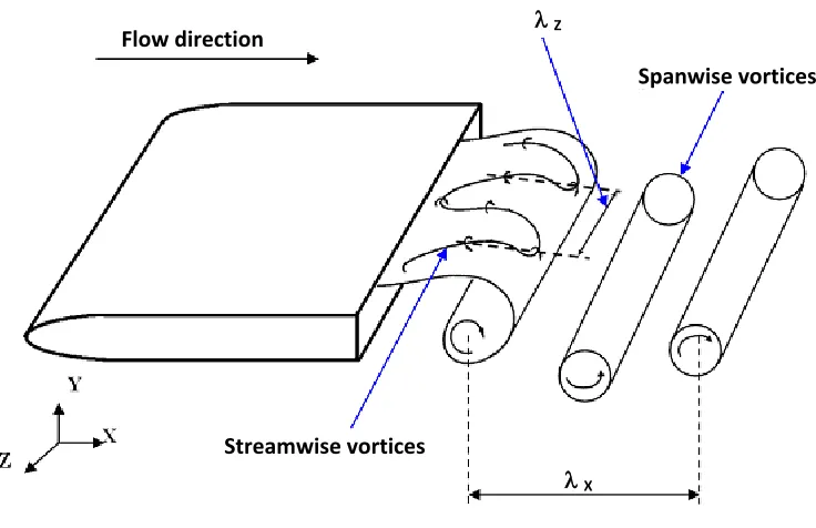
Wake flows behind nominally two-dimensional bodies are dominated mainly by two

types of coherent structures, namely the Karman Benard spanwise vortices and the

streamwise vortices (Figure 1-2), also referred to as rolls and ribs respectively. It has

been established that ribs wrap around rolls, and are interconnected (Hussain and

(26)

Hayakawma 1987). Development of two- and three-dimensional instabilities in the near

wake of a two-dimensional body is sensitive to external actuation, which can be used in

the design of control strategies to mitigate vortex shedding and minimize lift fluctuations

and drag (Tombazis and Bearman 1997; Darekar and Sherwin 2001; Julien et al. 2003;

Dobre et al. 2006; Lam and Lin 2009). Identifying the most unstable secondary wake

instability and triggering it would be the most efficient way to develop a wake control

mechanism. The present work is a step towards the longer term goal of developing a

robust wake control methodology based on the manipulation of streamwise vortices as a

function of Reynolds (Re) and Strouhal (St) numbers for blunt trailing-edge-profiled

bodies. In essence, the normalization proposed by Dobre et al. (2006) for different wake

generators is extended as

 

z_x  Dz.St

(

1.1) Flow direction

Streamwise vortices

Spanwise vortices

X

Z

(27)

where xandzare the streamwise spacing between the consecutive rolls and the

spanwise spacing between the consecutive ribs, respectively (Figure 1-2), and D is the

thickness of the wake generator.

The following sections review the literature on three-dimensional near wakes and

passive flow control using Spanwise Sinusoidal Perturbation (SSP), and identify

background work motivating the present study and specific objectives of the

experimental work.

1.1 Previous Studies on Three-Dimensional Near Wakes

It is only in the last two decades that research has been conducted on the

three-dimensional near wake flow topology for various wake generators, such as circular

cylinders (Karniadakis and Triantafullou 1992; Bays-Muchmore and Ahmed 1993; Mansy

et al. 1994; Zhang et al. 1995; Brede et al. 1996; Williamson 1996; Barkley and

Henderson 1996), square cylinders (Robichaux et al. 1999; Luo et al. 2003; Dobre and

Hangan 2004; Luo et al. 2007; Sheard et al. 2009), thin flat plates (Meiburg and Lashares

1988; Julien et al. 2003), blunt trailing-edge-profiled body (Ryan et al. 2005), bluff rings

(Sheard et al. 2005), and blunt trailing edge airfoil (El-Gammal and Hangan 2008).

The near wake of a two-dimensional body is critical because of dominant primary

instability, which leads to the vortex street formation (Unal and Rockwell 1988). For

circular cylinders, this bifurcation occurs at the critical Reynolds number of Rec45. Further transition in the near wake is responsible for the formation of three-dimensional

secondary instabilities, leading to the turbulent state, experimentally investigated by

Williamson (1996) and numerically by Barkely and Henderson (1996). According to these

studies, the transition from two- to three-dimensional instabilities occurs for a wide

range of Reynolds numbers from Rec 140 to 190. The possible reason for this variability is that the background disturbances are influencing the critical Reynolds

number (Rec) (Unal and Rockwell 1988). Other factors such as aspect ratio (height to

(28)

influence Rec (Prasad and Williamson 1997). Williamson (1996) demonstrated that for

circular cylinder flows, two distinct three-dimensional streamwise instability modes

occur, specifically mode-A and mode-B, depending on the flow Reynolds numbers.

Mode-A occurs at ReD > 180, ReD being the Reynolds number based on the thickness of

the wake generator, and is gradually replaced by mode-B at ReD > 230. The spanwise

spacing between streamwise vortices of Mode-A is scattered between 4D and 5D

(Williamson 1996), but for Mode-B it is consistently found to be around 1D (Williamson

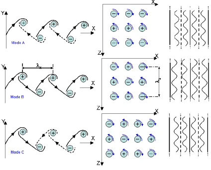
1996) for various Reynolds numbers. The spatio-temporal symmetries of mode-A and

mode-B are shown in Figure 1-3. For mode-A, the region of positive and negative

streamwise vorticity alternates in the spanwise direction and with time. The sign of

(29)

streamwise vorticity, and thereby direction of the secondary vortices, alternates twice

every Karman cycle. For mode-B, the streamwise vorticity pattern shows spanwise

periodicity. Yet in contrast to mode-A, the sense of rotation does not change with time

for a given spanwise location. Furthermore, the secondary vortices of mode-B seem to

be persistent in time and remain connected over many Karman cycles. The entire

patterns of secondary vortices oscillate up and down sinusoidally during each cycle of

Karman vortex formation. Zhang et al. (1995) showed that a third mode, mode-C,

appears when the flow is forced externally using an interference wire very close to the

cylinder. Mode-C appears with a spanwise wavelength of 2.0D. For this mode, the

vorticity direction of streamwise vortices connecting the spanwise vortices alternates

every Karman vortex cycle at a particular spanwise location with time (Figure 1-3).

However, the full Floquet stability analysis of an unforced cylinder wake by Barkley and

Henderson (1996) captures only mode-A and mode-B instabilities. Hence, it can be

inferred that other three-dimensional instabilities can be triggered with suitable forcing.

For a square cylinder, Robichaux et al. (1999) conducted low ReD numerical

simulation based on Floquet analysis. They found the same natural modes with larger

spanwise spacing of 5.22D for Mode-A and 1.2D for Mode-B. Luo et al. (2003, 2007)

made a similar type of observation from the PLIF and PIV measurements. Robichaux et

al. (1999) also predicted a third instability mode, mode-S, with a spanwise spacing of

2.8D. This mode has similar features to mode-C observed by Zhang et al. (1995). As

opposed to mode-C, however, mode-S naturally evolves in the flow without any external

forcing. While Robichaux et al. (1999) inferred that mode S is subharmonic, with periodic

double of the base flow, Blackburn and Lopez (2003) demonstrated that it is not true

subharmonic but repeats every second cycle. Dobre and Hangan (2004) proposed a

structure similar to Mode-A with a spanwise spacing of 2.4D at high Reynolds numbers

(ReD = 22000) in the intermediate wake of the square cylinder.

Mieburg and Lashares (1988) and Julien et al. (2003) experimentally studied the

dynamics of three-dimensional secondary instabilities developing in the wake of a thin

(30)

with a spanwise wavelength z/x = 1, whereas in the far wake both modes (mode-A and

mode-B)coexist and grow equally.

It appears that the wake of two-dimensional bluff bodies undergoes transition to

three-dimensional flow and eventually turbulence, through the same sequence of

transition as observed for circular cylinder (Williamson 1996), and that mode-B

dominates the flow after a certain transition Reynolds number. Previous studies on

square cylinder (Robichaux et al. 1996; Luo et al. 2003; Luo et al. 2007) and thin flat

plate (Mieburg and Lashares 1988; Julien et al. 2003) support this assumption, but with a

slight variation in the spanwise spacing of these instabilities. However, for blunt

trailing-edge-profiled bodies, Ryan et al. (2005) showed that when aspect ratio (AR) < 7.5, the

flow transition to three-dimensionality is through mode-A and mode-B respectively, and

that mode-A instability dominates the near wake development. For intermediate and

long bodies (AR > 7.5), the flow transition to three-dimensionality is through mode-B

first and then through mode-A at higher Reynolds number, while mode-B instability

plays a dominant role in the near wake dynamics. They reported a spanwise spacing

(z/D) of 3.5 for Mode-A and of 2.2 for Mode-B. They also observed a third instability

mode, mode S, with a similar spatio-temporal structure to mode-C, but with a spanwise

spacing of the order of one diameter (spacing similar to mode-B instability in circular

cylinder flows). Adding further support to this argument, Sheard et al. (2005) confirmed

that the near wake flow of a bluff ring is dominated by sub-harmonic three-dimensional

instability mode-C. Sheard et al. (2009) also demonstrated that the transition to

three-dimensional flow in the near wake of a square cylinder with variation in incidence

angles, mode-A instability or mode-C instability dominated the flow structure. When

studying the flow around two cylinders in a staggered arrangement, Carmo et al. (2008)

showed that mode-C is also present along with mode-A and mode-B, depending on the

relative position of the cylinders.

In summary, the transition to three-dimensional flow and the corresponding

instabilities, which are mode-A, mode-B, mode-C or mode S, may vary in terms of the

(31)

preferred spanwise wavelength associated with streamwise vortices is not clear. While

some researchers indicate that spanwise wavelength is broadband (Mieburg and

Lashares 1988; Julien et al. 2003; Ryan et al. 2005), being imposed by the upstream

conditions, others have shown evidence of a preferred natural spanwise wavelength

(Zhang et al. 1995; Williamson 1996; Robichaux et al. 1999). The preferred spanwise

wavelength is rather scattered, and is explained by the presence of ribs or by the

spanwise roll distortions or both. However, it appears that the preferred spanwise

wavelength is a function of flow configuration, meaning geometry (Ryan et al. 2005;

Sheard et al. 2005; Sheard et al. 2009; Carmo et al. 2008), and aspect ratio (Ryan et al.

2005) of the wake generator, inflow conditions such as the Reynolds number, and

turbulence characteristics (Williamson 1996; Wu et al. 1996).

1.2 Previous Studies on Flow Control Using Spanwise Sinusoidal

Perturbation (SSP)

The control of vortex shedding in the wake of the bluff bodies by both active and

passive means has been extensively investigated. Gad-el-Hak et al. (1998) provided a first

comprehensive review. Passive control is reliable because of simplicity and cost

effectiveness, and hence, is often preferred over active control methods. Successful

passive control of vortex shedding in bluff bodies has been obtained with splitter plates

(Bearman 1965), base bleed (Bearman 1967), three-dimensional disturbances (Tanner

1972), surface protrusions (Zdravkovich 1981), segmented trailing edges (Petrusma and

Gai 1996), wavy trailing edges (Tombazis and Bearman; 1997, El-Gammal 2007), wavy

leading edges (Bearman and Owen 1998; Darekar and Sherwin 2001; Dobre et al. 2006),

and vortex generators (Park et al. 2006; El-Gammal 2007).

The control of vortex shedding by application of Spanwise Sinusoidal Perturbation

(SSP) has recently gained interest because of its simplicity in design and its applicability

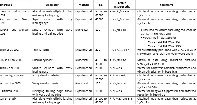
to different wake generators (see Table 1.1). SSP control has been successfully applied to

(32)

Lin2009), square cylinders (Bearman and Owen 1998; Darekar and Sherwin 2001; Dobre

et al. 2006), elliptic leading and blunt trailing edge body (Tombazis and Bearman 1997),

and divergent trailing edge airfoil (El-Gammal 2007). Table 1.1 summarizes most of these

investigations. The literature indicates that there is no preferred spanwise wavelength

that is common across various geometries. Several researchers (Darekar and Sherwin

2001; Kim and Choi 2005; Dobre et al. 2006) have indicated that maximum reduction in

the dynamic loads and suppression of vortex shedding were obtained when the

perturbation length was close to the spanwise spacing of the secondary wake

instabilities. Three-dimensional wake instabilities lead to distinct instability modes

(mode-A, mode-B and mode-C/mode-S) depending on the flow Reynolds number,

Strouhal number and shape of the wake generator (Zhang 1995; Williamson 1996;

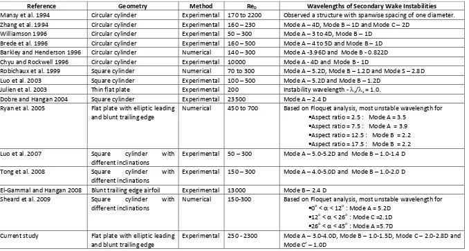
Robichaux et al. 1999). Drawing on previous studies, Table 1.2 summarizes the spanwise

spacing of the secondary wake instabilities for various wake generators. The spanwise

spacing of the secondary wake instabilities varies with geometric shape, aspect ratio and

Reynolds number. Based on the information from Table 1.1 and Table 1.2, it appears

that, for a circular cylinder, the maximum base drag reduction using SSP control (Kim and

Choi 2005; Lee and Nguyen 2007; Lam and Lin 2009) is obtained at wavelengths of 2.0 to

2.5D and of 5D to 6D. These wavelengths are very close to the wavelengths of the

instabilities of the near wake observed for a circular cylinder. While mode-C with a

spanwise wavelength of 2.0D does not occur naturally, Zhang et al. (1995) showed that

this mode appears in the presence of an interference wire placed close to and parallel to

the cylinder axis. The 5.0D wavelength corresponds to the naturally occurring mode-A

instability. For a square cylinder, the maximum base drag reduction (Bearman and Owen

1998; Darekar and Sherwin 2001; Dobre et al. 2006) is obtained at wavelengths of 5.6D

and 2.4D, which are close to naturally occurring instability wavelengths of mode-A (5.2D)

and mode-C (2.8D). El-Gammal (2007) showed that vortex shedding can be suppressed,

and achieved maximum base drag reduction for a diverging trailing edge airfoil by

perturbing the near wake with the spanwise wavelength of the secondary wake

(33)

Reference Geometry Method ReD _wavelengthsTested Comments

Tombazis and Bearman 1997

Flat plate with elliptic leading and wavy trailing edge

Experimental 20000 to 60000

3.5 < z/D < 5.6 Obtained maximum base drag reduction at

_z/D = 3.5 Bearman and Owen

1998

Square cylinder with wavy leading edge

Experimental 40000 3.5 < z/D < 5.6 Obtained maximum base drag reduction at

z/D = 5.6

Darekar and Sherwin 2001

Square cylinder with wavy leading and trailing edge

Numerical 100 0 < z/D < 10 Obtained maximum base drag reduction at

z/D = 5.6 and W/z=0.03

Fluctuating lift was zero for

z/D = 2.8 and W/z=0.2

z/D = 4.0 and W/z=0.06

Julien et al. 2003 Thin flat plate Experimental 200 0.5 < z/x < 1.1 When instability perturbed with z/x = 0.76, it

grew much faster than any other wavelength

Kim and Choi 2005 Circular cylinder Numerical 40 to 3900

2 < z/D < 10 Maximum base drag reduction obtained

withz/D = 4.0 to 5.0

Dobre et al. 2006 Square cylinder with wavy leading edge

Experimental 23500 z/D = 2.4 Vortex shedding was completely mitigated and

observed reduction in base drag Lee and Nguyen 2007 Wavy circular cylinder Experimental 5000 to

20000

z/D = 1 and 2 Obtained maximum base drag reduction at

z/D = 2.0

Lam and Lin 2009 Wavy circular cylinder Numerical 100 1 <z/D < 10 Obtained maximum base drag reduction at

z/D = 2.5 and 6.0

El-Gammal 2007 Diverging trailing edge airfoil with wavy trailing edge

Experimental 13000 z/D = 2.4 Vortex shedding was suppressed and observed

reduction in base drag Current study Flat plate with elliptic leading

and wavy trailing edge

Experimental 24000 to 46000

z/D = 2.4 and 5.6 Obtained maximum base drag reduction at

z/D = 2.4

(34)

Reference Geometry Method ReD Wavelengths of Secondary Wake Instabilities Mansy et al. 1994 Circular cylinder Experimental 170 to 2200 Observed a structure with spanwise spacing of one diameter. Zhang et al. 1994 Circular cylinder Experimental 160 – 230 Mode A – 4D, Mode B – 1D and Mode C – 2D

Williamson 1996 Circular cylinder Experimental 50 – 300 Mode A – 3 to 4D, Mode B – 1D Brede et al. 1996 Circular cylinder Experimental 160 – 500 Mode A – 4 to 5D and Mode B – 1D Barkley and Henderson 1996 Circular cylinder Numerical 140 – 300 Mode A -3.96D and Mode B - 0.822D Chyu and Rockwell 1996 Circular cylinder Experimental 10000 Mode A - 4D and Mode B - 1D

Robichaux et al. 1999 Square cylinder Numerical 70 to 300 Mode A – 5.2D, Mode B – 1.2D and Mode S – 2.8D Luo et al. 2003 Square cylinder Experimental 100 – 500 Mode A – 5.2D and Mode B – 1.2D

Julien et al. 2003 Thin flat plate Experimental 200 Instability wavelength - z/x = 1.0.

Dobre and Hangan 2004 Square cylinder Experimental 23500 Mode A – 2.4 D Ryan et al. 2005 Flat plate with elliptic leading

and blunt trailing edge

Numerical 450 to 700 Based on Floquet analysis, most unstable wavelength for Aspect ratio = 2.5 : Mode A = 3.5

Aspect ratio = 7.5 : Mode A = 3.9 Aspect ratio = 12.5 : Mode B = 2.2 Aspect ratio = 17.5 : Mode B = 2.2 Luo et al. 2007 Square cylinder with

different inclinations

Experimental 50 – 300 Mode A – 5.0-5.2D and Mode B – 1.0-1.4 D

Tong et al. 2008 Square cylinder with different inclinations

Experimental 150 – 300 Mode A – 4.0-5.0D and Mode B – 1.0-2.0 D

El-Gammal and Hangan 2008 Blunt trailing edge airfoil Experimental 13000 Mode B – 2.4 D Sheard et al. 2009 Square cylinder with

different inclinations

Numerical 150-300 Based on Floquet analysis, most unstable wavelength for 0o <  < 12o : Mode A = 5.2D

12o <  < 26o : Mode C =2.1D 26o <  < 45o : Mode A =5.7D Current study Flat plate with elliptic leading

and blunt trailing edge

Experimental 250 - 2300 Mode A – 3.0-4.0D, Mode B – 1.0-1.5D, Mode C – 2.0-2.8D and Mode C’ – 1.0D

(35)

current study, Ryan et al. (2005) showed that the spanwise wavelengths characterizing

the instabilities change with aspect ratio. Tombazis and Bearman (1997) investigated an

elliptic leading edge and blunt trailing edge body with an aspect ratio of 6.3, and

obtained maximum base reduction with a perturbation wavelength of 3.5D. This

wavelength closely matches the wavelength of the dominant instability of 3.9D for this

aspect ratio (Ryan et al. 2005). In the current study, an elliptic leading edge and blunt

trailing edge body is studied with an aspect ratio of 12.5 and obtained maximum base

drag reduction with a perturbation wavelength of 2.4 D, which closely matches the

wavelength of the dominant instability of 2.2D for this aspect ratio (Ryan et al. 2005). In

summary, there is a clear correlation between the waviness of the spanwise sinusoidal

perturbation (SSP) and the spanwise wavelength of the near wake instabilities. This

information is used in the current study to design the passive flow control.

1.3 Motivation and Objectives

Two important reasons for choosing flat plate geometry with profiled leading and

blunt trailing edge are: (i) it provides the desired upstream boundary layer velocity

profile at the trailing edge without the uncontrollable effects of forced

separation-reattachment associated with sharp corners of a square leading edge; and (ii) this

geometry is of particular interest for aeronautical transonic divergent trailing edge

airfoils (DTE), as well as for truncated wind turbine blade airfoils. The main outcome

relates to the development of flow control strategies based on the natural flow

instabilities.

The geometry used in the current study has been numerically investigated by Ryan

et al. (2005) in a Reynolds number range of 250 to 700 for aspect ratios of 2.5, 7.5, 12.5

and 17.5. Numerical modeling was performed in two stages. First a time-dependent

two-dimensional flow field around the blunt trailing edge profiled body is predicted by

solving the time-dependent Navier-Strokes equations in two dimensions. Above a

(36)

familiar periodic flow field of Karman vortex street with a period T. The stability of this

periodic two-dimensional base flow field to three-dimensional disturbances is then

determined using Floquet stability analysis. Table 1.3 summarizes the observations from

this work; it shows that the order of appearance of the near wake three-dimensional

secondary-wake instabilities depends on the aspect ratio. The researchers reported that

mode-A wake instability dominates the near wake development when AR < 7.5, with a

spanwise wavelength of 3.5D to 3.9D and by mode-B for AR > 7.5 with a spanwise

wavelength of 2.2D. Their study, however, is limited by the capability of the linear

stability analysis to predict the transition regimes for higher Reynolds number. There has

been no experimental verification of these numerical findings reported in the literature,

and therefore this constitutes one of the objectives of the current investigation. The

scope of the current investigation is as follows:

 Perform well-controlled experiments using Planar Laser Induced Fluorescence (PLIF)

and Particle Image Velocimetry (PIV) to verify the findings of the numerical work by

Ryan et al. (2005) for the same geometry with an aspect ratio of 12.5.

 Extract the dominant coherent structures by performing Proper Orthogonal

Decomposition (POD) on the obtained PIV data, and relate the POD modes and

associated eigenvalues to the dominant coherent structures in near wake.

 Identify the spatio-temporal topologies of the near wake instabilities and their

corresponding unstable wavelengths.

Aspect Ratio (AR) 1st Instability mode 2nd Instability mode 3rd Instability mode

2.5 Mode A – 3.5D

(ReD = 400)

-- --

7.5 Mode A – 3.9D

(ReD 470)

Mode B – 2.2D (400 < ReD < 500)

Mode C – 0.9-1.0D (ReD>500) 12.5 Mode B – 2.2D

(ReD 410)

Mode A – 3.5D (ReD 600)

Mode C (ReD > 600) 17.5 Mode B – 2.2D

(ReD 430)

Mode C – 0.7D (ReD 690)

Mode A – 3.5D (ReD > 700)

(37)

 Extend the study to higher Reynolds numbers, check whether modes-A, -B and -C

coexist, and identify which instability mode dominates the near wake development.

 Use these three-dimensional near wake dynamics to formulate a wake control

methodology.

 Demonstrate the effectiveness of this control methodology by testing a simple

passive control using Spanwise Sinusoidal Perturbation (SSP) with a design based on

(38)

2 EXPERIMENTAL SETUP AND ANALYSIS APPROACH

The wake dynamics of a blunt trailing-edge-profiled body, with and without the SSP

passive control, is investigated in the current study using surface base pressure, Particle

Image Velocimetry (PIV), and Planar Laser Induced Fluorescence (PLIF) techniques. In

order to explore the influence of the inlet conditions and Reynolds number, and check

the robustness of the proposed control methodology, experiments were conducted in

two different facilities: Low Reynolds number PLIF and PIV measurements were

conducted in the water tunnel of The Boundary Layer Wind Tunnel Laboratory at The

University of Western Ontario, and high Reynolds simultaneous surface base pressure

and PIV measurements were conducted in the wind tunnel at the University of Wyoming

Aeronautics Laboratory. This chapter describes these two facilities, the PLIF, PIV, and

pressure systems employed, as well as the data acquisition and primary processing.

2.1 Experimental Facility

2.1.1 Water Tunnel Facility

All the experiments for low Reynolds numbers (250 to 2300) were conducted in the

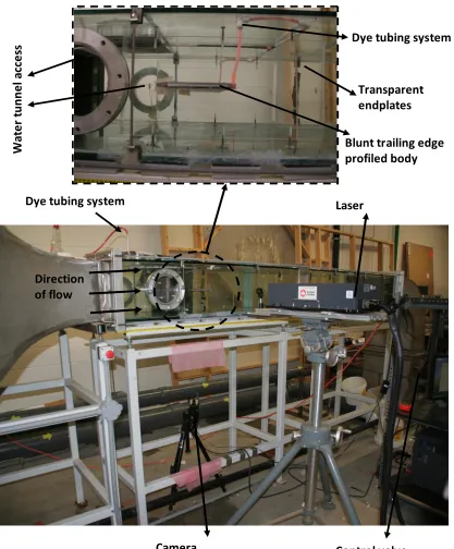
0.61 m x 0.305 m x 3 m water tunnel facility at The Boundary Layer Wind Tunnel

Laboratory at the University of Western Ontario. Figure 2-1 shows the water tunnel

experimental setup. This is an open return water tunnel producing a maximum

free-stream velocity of 0.2 m/s. The water introduced into the water tunnel, passes through a

settling chamber consisting of honeycomb and screens to break down large-scale

non-uniformities. Access inside the water tunnel is provided from the side walls of the test

section through two openings as shown in Figure 2-1. The model is supported using two

aluminum rails attached to the side walls of the test section. There is also an access

(39)

Laser

Camera

Blunt trailing edge profiled body

Dye tubing system

Transparent endplates

W

at

e

r

tu

n

e

l a

cc

e

ss

Dye tubing system

Direction of flow

Control valve

Figure 2-1 Water tunnel experimental setup

velocity in the water tunnel is controlled by a control valve situated at the end of test

(40)

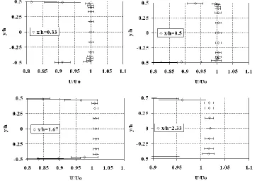
Figure 2-2 shows the mean streamwise velocity variation at the centre line of the

water tunnel at different downstream locations (reproduced with permission from Sarathi

2009). It is observed that the mean streamwise velocity profile is uniform and the

maximum variation in the mean velocity varies within 1%. The increase in the mean

streamwise velocity with downstream location, an effect of the boundary layer

development in downstream, represents only 0.5% variation in the mean streamwise

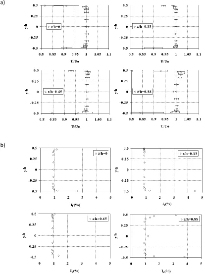
velocity over the extent of the measurement region downstream (2.1 < X/h < 2.4). Figure

2-3 shows the variation of (a) mean streamwise velocity and (b) turbulence intensity

variation at different spanwise locations at X/h = 0.33. The variation in the mean

streamwise velocity and the turbulence intensity is uniform across the span up to Z/h =

0.65. However, at Z/h = 0.88, the effect of the boundary layer growing on the side walls is

visible in these profiles. For the current experiments, the measurements were performed

in the water tunnel at 2.1 < X/h < 2.4, -0.04 < Y/h < 0.04 and -0.09 < Z/h < 0.09. It is

observed that the maximum variation in the mean velocity varies within 0.5% and that the

(41)

(a)

(b)

(42)

turbulence intensity is approximately 0.9% across the span where the measurements are

performed.

2.1.2 Wind Tunnel Facility

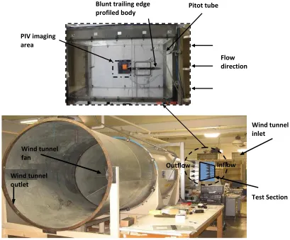
All the wind tunnel experiments for this investigation were conducted in the

subsonic wind tunnel facility (Figure 2-4) at the University of Wyoming Aeronautics

Laboratories (UWAL) using a 0.61m x 0.61m x 1.21m test section. This is an open loop

wind tunnel with a Variable Frequency Driven (VFD) motor capable of producing

free-stream velocities between 10 and 50 m/s. The inlet section of the wind tunnel has a

Flow direction Pitot tube

Blunt trailing edge profiled body

PIV imaging area

Wind tunnel outlet

Wind tunnel fan

Test Section Wind tunnel inlet

Inflow Outflow

(43)

honeycomb insert and three sets of screens to break down large-scale non-uniformities.

For easy access and to provide support to the models, the side walls of the test section

have been designed in two pieces. The two pieces of the side wall are made of plexiglass,

as shown in Figure 2-4. The plexiglass section provides access to perform various optical

measurements in the near wake of the models. Furthermore, there is a small window

section on the plexiglass through which wires and tubes may be routed out of the test

section for instrumentation and pressure measurements, respectively. The desired

free-stream velocities are achieved using a Proportional Integral and Differential (PID)

feedback control system. The input signal for the close-loop feedback system comes

from a pitot tube installed in the upstream test section of the wind tunnel. A LabView

program processes the input signal using the PID feedback control scheme and sends the

final output control signal (0-10V) to the VFD, which controls the motor driving the fan.

(a) (b)

Figure 2-5 Variation of (a) mean streamwise velocity and (b) turbulence intensity profile in the boundary layer at X/D = 0.4 before separation

Figure 2-5 shows the streamwise velocity and the turbulence intensity profile

developing in the boundary layer of the flat plate, just before separation at X/D = 0.4.

The profiles indicate that the development of the mean streamwise velocity is uniform,

the free-stream turbulence intensity being approximately 0.9%. Higher turbulence

intensity very close to the wall of the flat plate is due to the sand strip used at the

(44)

2.2 Models

This investigation uses a flat plate model with an elliptic leading edge and blunt

trailing edge to study

 the near wake dominant coherent structures, and

 the receptivity of spanwise sinusoidal perturbation with different spanwise

wavelengths.

To cover an extensive range of Reynolds numbers and to check the influence of

different inflow conditions, measurements were performed in both the water and the

wind tunnel. The details of the models used in the current investigation are discussed in

the following sections.

2.2.1 Water Tunnel Model

The fore-body length (Lx), spanwise length (Lz), and the base height (D) of this model

are 0.1587m, 0.6m and 0.0127m respectively. The actual measurements were

performed over a span of 0.43 m, which is bounded by two transparent endplates made

of plexiglass (Figure 2-6). The endplates isolate the body from the effects of the

boundary layers on the sidewalls of the tunnel, as well as from the dye supply tubing

system. The effective aspect ratio Lx/D of the model is 12.5, and Lz/D is 34, with a

blockage ratio of 4.2%. The important model dimensions along with the coordinate axis

used are shown in Figure 2-6. The X-axis is the streamwise direction, the Y-axis is the

transverse direction, and the Z-axis is the spanwise direction. The model covers the

entire spanwise length of the wind tunnel, thereby achieving quasi two-dimensional

flow over the model. The fluorescent dye was introduced into the flow through a thin

spanwise slot (0.5mm) on the lower surface of the body, located 1D upstream of the

(45)

Transparent end plate Flow direction

Elliptic leading edge

Imaging Planes

LX = 12.5D

Lz = 48D

D = 0.0127 m

Z X

Y

Dye injection slot

34D

(46)

2.2.2 Wind Tunnel Model

The fore-body length (Lx), spanwise length (Lz) and the base height of this model are

0.3175m, 0.61m and 0.0254m respectively. The aspect ratio Lx/D of the model is 12.5

and Lz/D is 24, with a geometric blockage ratio of 4.2%. A 0.012m wide sand strip is

applied along the leading edge to ensure that the boundary layer is fully turbulent on

the model. This was not used in the water tunnel as transition effects were of interest.

Important model dimensions along with the coordinate axis used are shown in Figure

2-7. The model covers the entire spanwise length of the wind tunnel, thereby achieving

quasi two-dimensional flow over the model. The model has pressure ports on the

fore-body as well as in the base region. The difference between mean pressure

measurements from the top and bottom surfaces of the fore-body is minimized to align

the model with the free-stream flow (that is, zero angle of attack). The pressure ports in

the base of the model (Figure 2-8) serve two purposes: first, they are used to measure

the base drag on the model, and second, they are used to calibrate the high-speed

transducers. The calibration of high speed transducers is discussed later in this chapter

(Section 2.3.3). PIV measurements were also performed on the flat plate model at

different vertical (XY) and horizontal (XZ) planes, as shown in Figure 2-7.

Three different trailing edges were used for this investigation. Two wavy trailing

edges with a spanwise wavelength (defined as the wavelength divided by base height)

Z/D = 2.4 and 5.6, with corresponding wave steepness (defined as the ratio of

peak-to-peak wave height divided by the wavelength) of W/z= 0.197 and 0.09, were tested, and

are referred to as SSP 2.4 and SSP 5.6 for the respective wavelengths. Details on

selection of the wavelengths of SSP are discussed in chapter 4. The third model has no

spanwise sinusoidal perturbation and will be referred to as the base case. The fore-body

length (Lx) for the wavy trailing edges is measured up to the half amplitude of the SSP as

shown in Figure 2-9, indicated with a blue dotted line, ensuring that the effective surface

(47)

Flow direction

Elliptic Leading edge LX= 12.5D

D = 0.0254m

X Y

Z

PIV Measurement planes Sand trip

Lz= 24D

Mean pressure taps

High speed pressure transducers

Figure 2-7 A schematic showing the flat plate model used in the wind tunnel, and the major dimensions along with the field of view for PIV images and the coordinate axis

(48)

W

MAX MIN

MED

Z

Straight trailing edge Sinusoidal trailing edge



Lx

Table 2.1 compares the dimensions of both the models and the tunnel dimensions

used in the current study.

Tunnel Dimensions (m) Model dimensions (m) Blockage ratio (%) Height Width length Lx Lz D AR

Lx/D Lz/D Water

Tunnel

0.305 0.61 3 0.1587 0.61 0.0127 12.5 48 4.2

Wind Tunnel

0.61 0.61 1.21 0.3175 0.61 0.0254 12.5 24 4.2

Table 2.1 Comparison of different dimensions of the tunnels and the models used in the study

2.3 Instrumentation

In order to achieve the objectives of this study, several experimental techniques

were used to characterize the near wake flow structure; these are discussed in the

following section.

Wake Dynamics and Passive Flow Control of a Blunt Trailing Edge Profiled Body

Scholarship@Western

Scholarship@Western

Wake Dynamics and Passive Flow Control of a Blunt Trailing Edge

Wake Dynamics and Passive Flow Control of a Blunt Trailing Edge

Profiled Body

Profiled Body

WAKE DYNAMICS AND PASSIVE FLOW CONTROL OF A BLUNT TRAILING

EDGE PROFILED BODY

THE UNIVERSITY OF WESTERN ONTARIO

THE SCHOOL OF GRADUATE AND POSTDOCTORAL STUDIES

CERTIFICATE OF EXAMINATION

WAKE DYNAMICS AND PASSIVE FLOW CONTROL OF A BLUNT TRAILING

EDGE PROFILED BODY

ABSTRACT

CO-AUTHORSHIP

ACKNOWLEDGEMENT

TABLE OF CONTENTS

LIST OF FIGURES

LIST OF TABLES

LIST OF SYMBOLS

1

INTRODUCTION

1.1

Previous Studies on Three-Dimensional Near Wakes

1.2

Previous Studies on Flow Control Using Spanwise Sinusoidal

Perturbation (SSP)

1.3

Motivation and Objectives

2

EXPERIMENTAL SETUP AND ANALYSIS APPROACH

2.1

Experimental Facility

2.1.1

Water Tunnel Facility

2.1.2

Wind Tunnel Facility

2.2

Models

2.2.1

Water Tunnel Model

2.2.2

Wind Tunnel Model



2.3

Instrumentation