Mathematical modelling of non-isothermal flow in buildings
Richard Lenhard1 and Tomáš Puchor1
1
University of Žilina, Faculty of Mechanical Engineering, Department of Power Engineering, Univerzitná 1, 010 26 Žilina, Slovakia
Abstract. Numerical simulations are used in many areas of science and technology. In last time are numerical methods used not only in small scale applications, in fluid mechanics, but are also used in civil engineering for simulation of air flow, for simulation of heat transfer. This paper deals with simulation of air flow in building for municipal use. The core of the paper is the calculation of the input parameters for the creation of numerical model and description of the model itself. The conclusion provides an analysis and comparison of simulation results with calculated values for the building.
1 Introduction
The numerical model is defined on the basis of various physical phenomena in complex differential equations. In this case, we will observe the flow of air in a rather complex geometry. In view of the fact that this is the 3D model of flow which can be described as a system of partial differential equations that can be solved by numerical methods. The calculation of the following equations are typically designed for a number of cells.
For the solution of ventilation can be used Fluent program, part of the software ANSYS package. When creating a numerical model it must be determined in the applicable geometry created with mesh computing. It is necessary to know all the input data and set them as boundary conditions that are necessary for correct calculation. After performing the calculation, it can be a graphical displayed of results.
In the numerical solution we choose a general model of the building. Another criterion was the choice of the ventilation system, the selected building should be ventilated with air to circulate. The layout of the proposed construction building is in Fig. 1. Numerical simulation is performed in order to determine if it is possible to achieve the natural air flow and the natural exchange of different combinations of open and closed windows and doors [1, 13] in the building.
2 Modeling and mesh computing
3D model of the building was made up from drawings for construction of the building. The model has been adapted and simplified to the need to perform CFD simulations.
Network is a systemic breakdown of computational domain into sub interlinked cells in 2D space or in 3D space [2].
For numerical simulation have been chosen, these mesh computing:
- hexagonal, - tetragonal, - polyhedral.
Table 1. Parameters of the building.
Building dimensions
Width 19 m
Length 22.6 m
Ground clearance 9.3 m
Area 343 m2
Volume 3,310 m3
Fig. 1 Building model geometry before treatment
Because it is a very complex model geometry the mesh must be created quickly. Of course computational mesh had to be of sufficient quality to get the best results from CFD simulations. [13]
2.1 Hexagonal mesh
geometry was aggravation elements toward the center of the volume of the model and to create a network composed of the elements of hexagonal and tetragonal.
Fig. 2 Cuts hexagonal mesh
Table 2. Parameters of a hexagonal mesh and quality
Mesh
Number of elements
Orthogonal Quality
Ortho Skew
Hexagonal
mesh 1,536,370 1.005.10
-12
0.999
2.2 Tetragonal mesh
Fig. 3 shows a network element tetragonal and was allowed automatically in the whole volume.
Fig. 3 Cuts tetragonal mesh
Table. 3. Parameters of a tetragonal mesh and quality
Mesh
Number of elements
Orthogonal Quality
Ortho Skew Tetragonal
mesh 5,484,930 3.125.10-2 0.955
2.3 Polyhedral mesh
Polyhedral mesh was made up of a mesh consisting of elements of tetragonal, as a command converting polyhedral fig. 4.
Fig. 4 Cut polyhedral mesh
Table 4. Parameters of a polyhedral mesh and quality
Mesh
Number of elements
Orthogonal Quality
Ortho Skew Polyhedral
mesh 1,137,173 1.059.10-1 0.894
Hexagonal mesh showed the worst quality mesh. Tetragonal mesh did not meet the quality or number of elements, but after converting to mesh polyhedral significantly decreased the number of elements and improve the quality of the mesh. For simulation was chosen polyhedral mesh.
3. Boundary conditions
Building has heated bench with a constant temperature at 36 °C and heated floor temperature at 25 °C. Outdoor design temperature is set to 15 °C. Design temperature for the walls is 5 °C. In the building will be simulated airflow with closed windows and doors at first. Based on simulation results, will be decided on whether the natural flow will be sufficient for air exchange in the building or installation of ventilation elements will be required [1].
In the programming environment of FLUENT have been set initial and boundary conditions. Among the software simulations, Ansys Fluent software allows, the simulation of physical and thermophysical effects to the greatest interface. Modeling airflow simulations were transferred by employing three models:
The procedure for entering the initial and boundary conditions were as follows:
1) input of material parameters,
2) enter the input and output values of the flowing medium,
3) set points,
4) adjusting the calculation, 5) initialization calculation, 6) start of calculation.
3.1 CFD simulation results
CFD simulation result is achieved by making the natural flow (Tab. 5) of air in the building. The resulting rates were compared with closed and open windows and doors using three calculation models.
Table 5. Scores air speed of CFD simulations
Velocity
[m.s-1] Simulation
Model open closed laminar 1.5253 3.5131
k- 0.1547 0.2282 k- 0.1403 0.4157
3.1.1 The results of numerical simulation model Laminar (open windows and doors)
Fig. 5 shows the temperature fields in laminar model. After completion of iterations can see the method and direction of mixing cold outside air with warmer air inside. Air distribution through building can be seen by streamlines and vectors of the air in the premises through the low-lying inlet openings (doors and windows) and exit through the skylight.
Fig. 5 Temperature ratio in laminar building model
Fig. 4 shows the different temperatures that range between – 14.8 °C to 25 °C in a church building section. Low visible mainly at the door and at the window 2, 5. Air temperature 25 °C is accumulated in the heated benches and rises to the ceiling.
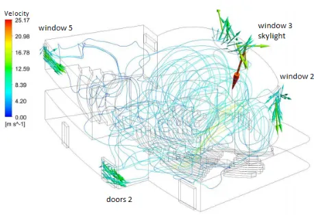
Fig. 6 Shows streamlines and the vectors in laminar model
Fig. 6 are shown the ventilation velocity laminar model; max. air velocity reaches 25.17 m.s-1. In the middle of the building can be seen mixing of air at lower speeds than the speed of the air inlet and outlet openings in each.
3.1.2 The results of numerical simulation model k-
Fig. 7 are shown the temperature fields in the model k-. In this model, the expiration of iterations was cold air entering through the lower area of the door and set down in the upper part of the door and the window and the window 1, 5. Also, you can see the temperature conditions through the headroom space. The movement of the nozzle and direction vectors is shown in Figure 8.
Fig. 7 Temperature ratio for model k-
k-3.1.3 The results of the numerical simulation model k –
The model k – was undesirable chimney effect-facing the flow of air inside the building, to a greater extent taking place thereto, and the skylight window of 3, and to a lesser extent through the open doors 2.
Fig. 9 Temperature ratio in the k – model
4 The results of numerical simulation
model Laminar (open windows and
doors)
The numerical simulation with closed windows and doors have been selected sections to display the contours of temperature and air velocity.
4.1 The results of numerical simulation model Laminar
Fig. 10 shows the internal temperature status with doors and windows closed as there is for heating the surrounding air from the benches on the ground floor and first floor and the air cooling of the walls.
Fig. 10 Temperature conditions in the model Laminar
Fig. 11 Velocity ratio for laminar model
4.2 Výsledky numerickej simulácie modelu k- a k–
Graphic documentation of the result of applying a numerical model to a -, in Fig. 12 and 14 are detected by the temperature fields in the building sections. Fig. 13 and 15 are the results of the speed range of flow shown by contours.
Fig. 12 Temperature ratio for model k-
Fig. 14 Temperature ratio for the k- model
Fig. 15 Velocity ratio for the k- model
5 Conclusion
Three types of meshes was created and compared after simulations.
The results of the comparison:
- A hexagonal network, increase magnification cell towards its center (the worst network). When reducing the number of components quality of network decreased.
- Tetragonal network was due to poor quality converted to grid "polyhedral", thereby reducing the number of components and quality of the network increased.
The result of the comparison network was chosen for simulation hexagonal grid and three models of turbulence "laminar", "k-", "realizable" of a wall with an extended feature "enhanced wall treatments" a model "for -standard". The simulations were carried out with closed and then opened selected windows and doors.
The main goal was to handle numerical simulation of flow in the building and pointing out that it is possible to perform such analyzes even before the position of the object itself.
Laminar model was best to simulate natural air flow through building.
Acknowledgement
This contribution is the result of the project: “Limits of radiative and convective cooling through the phase
changes of working fluid loop thermosiphon”; APV 15 0778
References
1. Daniels, K.: Technika budov - Príruþka pre architektov a projektantov. Bratislava: Jaga grup, s. r. o., (2003).
2. ANSYS Help. 2015 Ansys Help Viewer 16.2. SAS IP, Inc. (2015).
3. Kaduchová, K., Lenhard, R., Gavlas, S., Jandaka, J.: The structural design of the experimental equipment for unconventional heating water using heat transfer surfaces located in the heat source, EPJ Web of Conf. 45, (2013).
4. Kaduchová, K., Lenhard, R., Gavlas, S., Jandaka, J.: Numerical simulation of indirect heating of water by heat transfer surface area located at the heat source, EPJ Web of Conf. 45, (2013).
5. Gatlin, E. Natural ventilation tricks to cool off your summer. [online].
6. Hehhálek, J. Spôsoby vetrania bytov a rodinných domov. [online].
7. uranský, P., Lenhard, R., Jandaka, J. Comparison of mathematical models for heat exchangers of unconventional CHP units. Acta Polytechnica: journal of advanced engineering, (2015).
8. Kasanický, M., Lenhard, R., Malcho, M. Optimization of atypical heat exchanger with using CFD simulation. Žilina, Transcom 2015, (2015). 9. Gavlas, S., uranský, P., Lenhard, R., Jandaka, J.
Mathematical simulation of heat exchanger working conditions. EPJ Web of Conference, (2015).
10. Kapjor, A., Hužvár, J., Ftorek, B., Smatanová, H. Analysis of the heat transfer from horizontal pipes at natural convection. AIP Conf. Proc. 1608, (2014). 11. Skoilasová, B., Skoilas, J. Determination of
pressure drop coefficient by CFD simulation. AIP Conf. Proc. 1608, (2014).
12. Siažik, J., Malcho, M, Rezniák, R.: Proposal of bypass in heat recovery system with sucking air, AIP Conf. Proc. 1745, (2016).
13. Lenhard, R., uranský, P.: Use of numerical simulation in building ventilation, XX. AEaNMiFMaE 2016, (2016)
14. Lenhard, R., Malcho. M.: The second device for measuring of the thickness of the falling condensate in the gravity assisted heat pipe. AIP Conf. Proc. 1745, (2016).
15. Kozubková, M., Šáva, P., Drábková, S.: Matematické modely nestlaitelného a stlaitelného proudní: metoda konených objem. Ostrava, (1999).