Numerical Analysis of Radar Response to Snow Using Multiple Backscattering Measurements for Snow Depth Retrieval

Numerical Analysis of Radar Response to Snow Using Multiple

Backscattering Measurements for Snow Depth Retrieval

Fatima Mazeh1, 2, *, Bilal Hammoud1, 2, 3, Hussam Ayad1, Fabien Ndagijimana2, Ghaleb Faour3, Majida Fadlallah1, and Jalal Jomaah1

Abstract—Study of snow is an important domain of research in hydrology and meteorology. It has been demonstrated that snow physical properties can be retrieved using active microwave sensors. This requires an understanding of the interaction between electromagnetic (EM) waves with natural media. The objective of this work is two-fold: to study numerically all physical forward models concerning the EM wave interaction with snow and to develop an inverse scattering algorithm to estimate snow depth based on radar backscattering measurements at different frequencies and incidence angles. For the first part, the goal is to solve the scattering calculations by means of the well-known electromagnetic simulator Ansoft High Frequency Structure Simulator (HFSS). The numerical simulations include: the effective permittivity of snow, surface scattering phenomena in layered homogeneous media (air-snow-ground) with rough interfaces, and volume scattering phenomena when treating snow as a dense random media. For the second part, the study is extended to develop a retrieval method to estimate snow thickness over ground from backscattering observations at L- and X-band using multiple incidence angles. The return signal from snow over ground is influenced by: surface scattering, volume scattering, and the noise effects of the radar system. So, the backscattering coefficient from the medium is modelled statistically by including a white Gaussian noise into the simulation. This inversion algorithm estimates first the snow density using L-band co-polarized backscattering coefficient at normal incidence and then retrieves the snow depth from X-band co-polarized backscattering coefficients using dual incidence angles.

1. INTRODUCTION

Seasonal snow has a great impact on the Earth’s climate system due to its high albedo. It can reflect 80 to 90 percent of the incident solar radiation back into space; thus, regulating the Earth’s energy balance. Moreover, one-sixth of the total population of the world depends on snowmelt runoff to meet their fresh water needs [1, 2] and for agricultural irrigation requirements [2]. In some drainage basins, rapid spring snowmelt may also cause flooding and thus predicting the runoff resulting from snowmelt which is an important part of the flood control system [2, 3]. That’s why there is a demand for an estimation of the snow depth as well as the snow water equivalent (SWE) in an accurate manner. In the last few decades, active microwave sensors have proven to be valuable tools in retrieving snow characteristics.

Remote sensing requires some electromagnetic theory study to obtain useful information from the sensor. To understand how microwave sensors operate and how electromagnetic quantities they measure are transformed into geophysical information, it is necessary to understand how EM waves interact with natural media [4]. Such interaction is called: scattering, absorption, transmission, and emission. The scattered electromagnetic energy from snow-covered ground measured by a radar depends on the

Received 28 April 2018, Accepted 15 June 2018, Scheduled 25 June 2018 * Corresponding author: Fatima Mazeh ([email protected]).

properties of snow as well as the properties of the radar itself such as: frequencyf, incidence angle θi,

and the polarization of the incident beam (H orV).

The study of snow depth retrieval has a long history. Many studies regarding snow physical properties retrieval methods are based on radar backscattering observations at different frequencies and polarizations. For example, an inversion algorithm of SWE using multi-frequency (L, C, X bands) and multi-polarization (V V and HH) microwave backscattering coefficients is represented by Shi and Dozier (2000) [3]. This inversion algorithm uses co- and cross-polarized channels for the separation of surface and volume scattering contributions and needs five measurements to estimate SWE. However, sensitivity analysis showed that backscattering signals at X-band or higher frequency bands is more sensitive to snow parameters than that at C-band. Hence, retrieving snow physical parameters at higher bands is more efficient. High frequency Synthetic Aperture Radar (SAR) (X and Ku band) with multi-polarization is proposed by the snow observation programs: the European space agency CoReH2O space borne synthetic aperture radar, and Snow and Cold Land Processes (SCLP) of NASA. SWE inversion algorithm under this configuration is done by [5, 6]. Ku-band is more sensitive to shallow snow only. So, the frequency choice is a compromise between how much it is capable to penetrate a deep snow layer meeting our requirements and how much it is sensitive to snow parameters. That’s why an operating frequency of 10 GHz was chosen in our retrieval method where a typical value of penetration depth into dry snow is around 8 m at such wavelength.

The main objective of this paper is the development of a snow depth inversion algorithm based on several backscattering observations. This requires an implementation of a MIMO (multiple input multiple output) radar which has the potential to operate at two frequencies and can scan multiple incidence angles simultaneously. The design of this high accurate sensor is left for future work. So, calculations were performed using Monte Carlo Simulations in MATLAB where the addition of a gaussian noise was just to reflect a similar data collected from a real radar. That’s why we use the statistical distribution of the backscattering coefficient under various snow depths, snow densities, and incident frequencies to retrieve snow depth.

The proposed algorithm requires some forward models for scattering from a ground layer and models regarding the snow density. Ansoft’s High Frequency Structure Simulator [7] (HFSS) was just a key to understand how electromagnetic waves are scattered by media and to choose the best fit forward model with the numerical results to use it in the snow depth retrieval algorithm. The study is then extended to develop a retrieval method to estimate snow density and thickness over ground from backscattering observations at L- and X-band using multi-incidence angles. This inverse scattering problem involves two steps. The first is the estimation of snow density using L-band co-polarized backscattering measurement at normal incidence. The second is the recovery of the snow depth from X-band radar backscattering coefficients using two incidence angles.

2. PROPAGATION PROPERTIES OF SNOW

Snow depth (d) and density (ρs) are two important parameters used to find out the snow water equivalent

(SWE). The snow water equivalent is a measure of the amount of water contained in a snowpack. This term is used in hydrology studies to predict snowmelt run-off. It is defined as:

SW E=dρs ρw

(1)

wheredis the snow depth (m); ρsis the snow density (kg/m3);ρwis the density of water (kg/m3) which

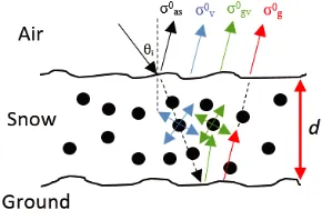
is constant for a specific temperature. As illustrated in Figure 1, the total backscatter σ_total0 received from snow above ground includes four scattering components:

σ0_total=σ0_as+σ_v0+σ_gv0 +σ_g0 (2) whereσ_as0 is the surface scattering component by the air/snow interface;σ0_v is the snow volume scattering due to ice inclusions; σ0_gv is the multiple scattering component involving both surface and volume scattering mechanisms; σ0_g is the surface scattering by the snow/soil interface. The backscattering coefficient is affected by: volumetric liquid water content in snowmv%, snow depthd, snow densityρs,

Figure 1. Scattering contributions for air-snow-ground multi-layered structure with rough interfaces and heterogeneous snow mixture.

The volume backscattering coefficient obeys the Rayleigh approximation for layers with small dielectric constant.

2.1. Single-Scattering Radiative Transfer Model with Rayleigh Particles (S2RT/R)

The total derived backscattering coefficient (σ_total◦ ) for a layer with a distinct upper boundary at polarizationpqis given by Equation (3). This formulation which is known as theS2RT /R[4] model will be used to simulate the surface and the volume backscattering coefficients of snow over ground (soil). Volume scattering is created by ice grains at the wavelengths comparable to the grain size.

σ_total,pq0 =T_pq2(θi)[Υ2pqσg,pq0 (θr) + 0.75acosθr(1−Υpq2 )(1 + Γ2g(θr)Υ2pq) + 6κsdΓg(θr)Υ2pq] +σas,pq0 (θi) (3)

whereTpq is the transmission from air to snow across the air-snow boundary; Υpq is the transmissivity

throughout the snow volume; ais the albedo; θi is the incidence angle; θr is the refraction angle; Γg is

the ground surface reflectivity; κs is the scattering losses; dis the snow depth. The transmissivity of

the snow layer can be expressed as:

Υpq = exp

− κed

cosθr

(4)

where κe is the extinction coefficient of the snow volume. The extinction coefficient accounts for

absorption and scattering losses within the snow as seen in Equation (5).

κe=κa+κs (5)

The scattering albedo is defined as:

a=κs/κe (6)

The volume absorption coefficientκais defined in terms of the effective permittivityεeff of the medium

and the wave numberk0 (k0 = 2π/λ) as shown in Equation (7). In the case where the size of inclusions

is much smaller than the wavelength λ,κs is much smaller thanκa (κe =κa).

κa=−2k0Im _√

ε_eff= 2πε

ds

λε_ds (7)

where ε_ds and ε_ds are the real and imaginary parts of the complex dielectric constant of snow, and quantify the electromagnetic energy stored and energy loss in the medium respectively.

2.2. Scattering Models

Many scattering models are available to simulate the ground surface backscattering coefficients under snow cover. Scattering models of terrain are, at best, good approximations of the true scattering process experienced by a real radar observing a real terrain surface or volume [4]. They serve as guides to explain experimental observations and as predictors of how the radar scattering coefficientσ0_{is likely to behave}

as a function of a particular terrain parameter of interest [4]. Some models are known as I2_{EM, PRISM,}

2.2.1. Polarimetric Radar Inversion for Soil Moisture (PRISM) Model

An empirical model was developed to measure the dielectric constant and moisture content of the soil medium by the University of Michigan team by Oh et al. (1992) [8] who developed the following empirical model:

p=σ_hh0 /σ0_vv =

1− 2θi π α

e−k0s

2

(8)

α = 1 Γ0

(9)

withsbeing the rms height of the surface and Γ0 representing the surface Fresnel reflectivity at normal

incidence:

Γ0=

1− √εsoil

1 +√εsoil

2 (10)

whereεsoil is the permittivity of the soil layer. The cross-polarized ratio is defined as:

q =σ0_hv/σ0_vv= 0.23Γ1₀/2

1−e−k0s ₍₁₁₎

Using the empirical models developed for p and q, the following models were developed for σ0_vv, σ_hh0 , and σ_hv0 :

σ_vv0 = 0.7

1−e−0.65(k0s)1.8cos3θi

√_p [Γv(θi) + Γh(θi)] (12a)

σ0_hh = pσ_vv0 (12b)

σ_hv0 = qσ0_vv (12c)

2.2.2. Soil Moisture Assessment Radar Technique (SMART) Model

Dubois et al. (1995) [9] developed a semi-empirical approach for modelling σ_vv0 and σ_hh0 named Soil Moisture Assessment Radar Technique (SMART) for soil moisture inversion. The algorithm is optimized for bare soils withk0s≤2.5, soil moisture ms≤35% andθi≥30◦.

σ_hh0 = 10−2.75·cos

1.5_θ

i

sin5θi

·100.028εsoiltanθi(k0ssinθi)1.4λ0.7 (13a)

σ0_vv = 10−2.35·cos

3_θ

i

sin3θi

·100.046εsoiltanθi_(k0ssinθi)1.1_λ0.7 _(13b)

whereε_soil is the real part of the soil dielectric constant.

2.2.3. Improved Integral Equation Model (I2EM)

The I2EM is applicable on a wide range of surfaces, from smooth to rough wherek0s <3 for a certain

radar wavenumber. The co-polarized backscattering coefficient equation according to [4, 10, 11]:

σ0_pp(θi) =

k2 0

4πe

−2k₀2s2cos2θi

∞

n=1

I_ppn 2W

(n)_(2k

0sinθi,0)

n! (14)

where

I_ppn = (2k0scosθi)fppexp(−k20s2cos2θi) + (k0scosθi)nFpp (15)

the following equations:

fhh = −

2Rh

cosθi

(16a)

fvv =

2Rv

cosθi

(16b)

Fhh = 2

sin2θi

cosθi

4Rh−

1− 1 εsoil

(1 +Rh)2

(16c)

Fvv = 2

sin2θi

cosθi

1− εsoilcos

2_θ

i

εsoil−sin2θi

(1−Rv)2−

1− 1 εsoil

(1 +Rv)2

(16d)

where the horizontally and vertically polarized Fresnel reflection coefficients,Rh and Rv, are given by:

Rh =

cosθi−

εsoil−sin2θi

cosθi+

εsoil−sin2θi

(17a)

Rv =

εsoilcosθi−

εsoil−sin2θi

εsoilcosθi+

εsoil−sin2θi

(17b)

Note that the expressions of these models assumes backscattering from an air/soil random rough surface. However, in our work, the ground is covered by a snow layer. That’s whyεsoil/εdsshould be used instead

of εsoil and θr should be used instead of θi when calculating the snow/soil interface backscattering

coefficient (σ_g0).

2.3. Wetness and Frequency

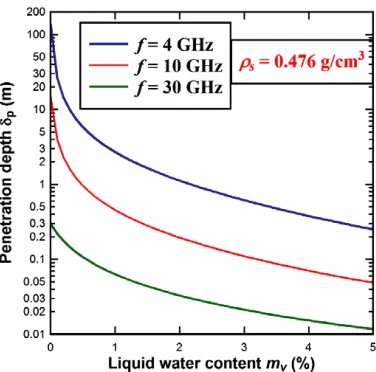
Penetration is a very important parameter for the remote sensing of snow. The possibility of information retrieval from the backscattered measures waves is dependent on how the EM wave is capable to penetrate a snow layer. It depends on the frequency of the incident EM wave as well as the dielectric constant of snow; that’s the liquid water content in snow. The more the liquid water content, the higher the dielectric constant, and therefore bigger absorption which means less penetration. That’s why wet snow attenuates the microwaves in a very short distance. The penetration depth (δp) is defined as [12]:

δp = 1/κe (18)

The extinction coefficient is computed using MIE solution [4]. Figure 2 shows the variation of the penetration depth (δp) for a snow layer as function of liquid water content (mv) for frequencies in

the microwave range. Snow physical parameters inversion algorithm at higher bands is more efficient, but higher bands means less penetration. The volume absorption coefficient increases as water content in snow increases, thereby no power is reflected, and hence the snow layer is not resolvable. This is illustrated well in Figure 2 which shows that a wet snow pack prevents reflection at higher frequencies.

2.4. Backscattering Behavior of Dry Snow

It is useful to study the backscattering behavior of dry snow before the snow depth estimation. The surface roughness of dry snow has almost no effect on the total backscattering coefficient due to the small dielectric contrast between air and dry snow (εair = 1 andεds = 1.9 for a density of 0.45 g/cm3). That’s

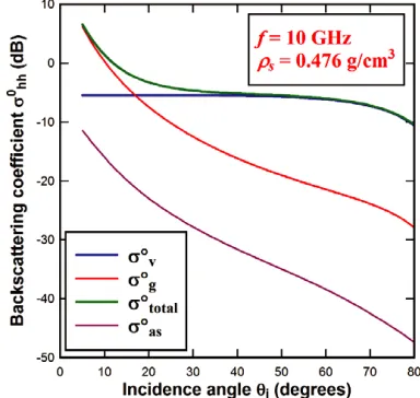
whyσ_as◦ could be neglected in the formulation given in Equation (3). This is in contrast to the wet snow case because of the high dielectric losses of liquid water. Furthermore, it is necessary to study the angular dependence of the total backscattering coefficient because the presented retrieval algorithm is based on the variation of the incidence angle. As it can be seen from Figure 3, the backscattering coefficient decreases with increasing incidence angle. This is due to the decreasing backscatter from the ground under snow. For small incidence angles, surface scattering is the dominating contribution. For higher incidence angles, volume scattering contribution becomes more significant. This is illustrated in Figure 4 where the total co-polarized backscattering coefficient is equal to the ground backscattering coefficient at angles less than 15◦. As incidence angle increases, the ground backscattering coefficient decreases and the total backscatter reflects the volume contributions. The plots are done for a 0.476 g/cm3 snow density which will be used in the application of the snow depth inversion algorithm because the median seasonal snow density in Lebanon over the 2-year period (2014–2016) was 0.476 g/cm3 [13].

Figure 3. The calculated backscattering coefficient as a function of the incidence angle at H-polarization.

Figure 4. Computations of the co-polarized volume, soil, and total backscattering coefficient separately.

3. SNOW PERMITTIVITY AND SNOW DENSITY ESTIMATION

loss dielectric, its imaginary part is much smaller than the real part (on the order of 10−4) which can be neglected in the forward scattering calculations with no significant effect on the results. As snow wetness increases, the real and imaginary part of the dielectric constant of snow increases. In the snow density and snow depth retrieval method, we consider dry snow only.

3.1. Effective Permittivity Forward Models of Dry Snow

In remote sensing applications, geophysical materials are often inhomogeneous and complicated in structure such as snow. The concept of the effective dielectric constant is an important tool in treating the interaction problem between electromagnetic waves and such complex material. An accurate estimation of the effective permittivity of snow is important in recovering the snow depth from the reflected signal toward the radar. The idea of the effective medium of an inhomogeneous material is to have an equivalent dielectric constant ε_eff such that the mixture responds to an electromagnetic excitation as if it is homogeneous. The mixing rules are often derived using static and quasi-static arguments assuming that the size of inclusions in the mixture is small compared to the wavelength of the incident electromagnetic field.

Dry snow is a two-phase mixture consisting of ice particles embedded in an air background. The ice inclusions in natural snow usually have a diameter of 0.1–2 mm [14], so the quasi-static assumption can be valid throughout the microwave range of dry snow. The dielectric constant of dry snow (εds=εds−jεds)

depends on the permittivity of air (εair), the permittivity of ice (εice = ε_ice−jε_ice), and the volume

fraction of ice vi. The volume fraction of icevi in snow is related to the snow density by:

vi =

ρs

0.9167 (19)

where 0.9167 g/cm3 is the density of ice. The real part of the permittivity of ice ε_ice is independent of frequency from 10 MHz to 300 GHz, and it exhibits a slight temperature dependence of the form [15]:

ε_ice= 3.1884 + 9.1×10−4T (−40◦C≤T ≤0) (20) whereT is the temperature in◦C. The temperature sensitivity toε_iceis very small and can be neglected; hence, the dielectric constant of dry snow ε_ds is also independent of temperature and frequency in the microwave region. Applying Polder-Van Santen (PVS) model to dry snow where air is the background medium and ice spheres are in the inclusions give:

εds−1

3εds

= vi(εi−1) (εi+ 2εds)

(PVS) (21)

Since ε_ice/ε_ice 1, the imaginary parts of εds and εi may be neglected when seeking an expression

forε_ds. Another mixing formula for ice spheres in an air background is the Tinga-Voss-Blossey (TVB) two-phase formula which provides a good fit to the experimental data shown in [16].

εds= 1 +

3vi(εi−1)

(2 +εi)−vi(εi−1)

(TVB) (22)

Moreover, an equally good fit to the data is provided by the empirical expression (Looyenga’s model) [3, 17]:

εds = 1 + 1.5995ρs+1.861ρ3s (Looyenga) (23)

3.2. Numerical Physical Modelling of Dry Snow

This section is intended to solve the direct problem in the effective permittivity calculations of snow by means of the well-known electromagnetic simulator (Ansoft HFSS). This FEM solver is able to calculate theS-parameters of the simulated structure from which we can calculate the effective permittivity. The simulation setup of dry snow can be seen in Figure 5. It is a cubic background of air of lengtha= 100 mm and permittivity 1 (εe = 1) where spherical ice inclusions (εice = 3.185 and dielectric loss tangent = 0)

are embedded in random positions occupying a volume fraction vi. Periodic boundary conditions were

(a) (b)

Figure 5. Schematics of the simulation setup. (a) The simulation model of dry snow with perfect electric boundary conditions. (b) The simulation model of dry snow with perfect magnetic boundary conditions.

as shown in Figure 5(a) while PMC (Perfect Magnetic Conductor) boundaries are assigned to the side faces in the y-direction as shown in Figure 5(b). The simulated fraction volume vi of ice varies from

0.01 to 0.5 because the density of dry snow is mostly below 0.5 g/cm3.

This setup is done for about 100 simulations of dry snow structure. In every simulation, the fraction volume and the positioning of inclusions were randomly chosen. Simulation is done for overlapped and non-overlapped spherical inclusions with a non-uniform size distribution respecting the quasi-static limit. Allowing spherical inclusions to overlap means that complex geometries can be formed. The geometry is then terminated and excited by two wave ports which compute the S-parameters. For permittivity simulations and snow density estimation, an operating frequency is chosen in the L-band spectrum (f = 2 GHz) so that snow grains are small compared to the incident L-band wavelength. This means that snow medium can act as a homogeneous dielectric layer with an effective permittivity.

For a plane wave normally incident on a homogeneous slab with thicknessd, theS21parameter for

a non-magnetic dielectric mixture can be expressed as follows [18]:

S21 =

(1−R2_)e−j√ε_effk₀d

1−R2_e−j2√ε_effk₀d (24)

R = (1− √ε_eff)/(1 +√ε_eff) (25) Note that Equation (24) is just a function containing one variableε_eff. Once theS parameters are computed, the effective permittivity can be calculated by solving the non-linear complex Equation (24).

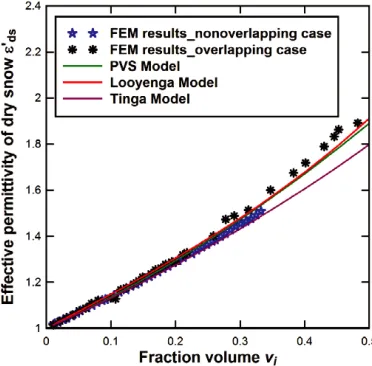
Figure 6 shows the effective permittivities achieved from 100 simulations from the FEM simulator for different volume fractions and positioning of inclusions. Each mixture has its own effective permittivity which may differ from another mixture having the same volume fraction of ice because of their different microstructure. The calculated permittivity distribution is also compared with the theoretical mixing models. It is shown that Looyenga’s model best fits the FEM simulated results in both cases: overlapped and non-overlapped inclusions. That’s why Looyenga’s model will be used in the snow density estimation method.

3.3. Numerical Simulation of Surface Scattering Effect in Layered Media with Rough Interfaces

Numerical simulation of electromagnetic scattering from a randomly rough surface has been a topic of successive study for many years because of its broad applications such as terrain remote sensing, radar surveillance over oceanic surface and so on [19, 20]. Numerical methods can calculate the exact scattered field by solving Maxwell’s equations so that the bistatic scattering coefficient can be determined.

3.3.1. Random Rough Surface Generation

The ability to generate a random rough surface to build a complex multilayered structure such as (air-snow-ground) with non-planar surfaces can improve our understanding of how electromagnetic waves are scattered by targets. A random rough surface is characterized by its: rms height (h), correlation length (cL), and auto correlation function (ACF). Electromagnetic models for scattering by random rough surfaces involve the use of the two most common forms for the correlation function: Exponential Correlation Function (ECF) and Gaussian Correlation Function (GCF). The two-dimensional random rough surface generation is solved in MATLAB and then imported into a CAD software to create the volume to be studied in an electromagnetic simulator. This procedure was developed because it is more flexible to use MATLAB generation instead of HFSS.

3.3.2. Procedure

For a rough surface being illuminated by a plane wave, the bistatic scattering coefficient for a single surface is defined as [21]:

γ_pq0 (θs, φs;θi, φi) = lim r→∞

4πr2 E_ps 2

_Ei q

2

Acosθi

(26)

In the backscattering direction θs = θi and φs = π +φi, the monostatic backscattering coefficient is

defined as:

σ_pq0 (θi, φi) = cosθiγpq0 (θs=θi, φs=π+φi;θi, φi) (27)

It is impossible to model an infinite rough surface numerically, so a procedure to do that is summarized in [22] where the bistatic scattering coefficient is averaged over N different rough surfaces with the same length L and the same roughness conditions. The scattered electric field by each rough surface is calculated in the far field region at a rangeRr from the surface as a function of the scattering

angle. This is done for N different rough surfaces with the same rms height and correlation length. Then, the bistatic scattering coefficient is averaged over the N surfaces for incident polarization p and scattered polarization q:

σ0_pq= 4πR

2

r

A Ei q 2 1 N N j=1

E_p,js 2 (28)

where A is the effective area of the rough surface. For a gaussian incident beam, the effective area is πg2_{/2 cos}2_{θ [23].}

In the averaging procedure, the choice of the surface lengthLis an important consideration in the numerical calculation. It is limited by conditions based on the wavelength λand the correlation length

For a finite surface, the plane incident wave leads to an edge effect on the circumference of the calculation area so that the calculated scattered field accuracy is reduced. That’s why tapered incident waves are applied in order to avoid artificial reflections from the edges of the illuminated finite surface by having a zero amplitude at the edges. A summary for the considerations regarding the choice of g and L are summarized in [20]. In most literatures, a value of g=L/4 is the most chosen choice in the averaging process. Calculations were done for 25 different surfaces (N = 25).

The HH-pol backscattering coefficient of a three-layered media is calculated where snow-soil interface is rough as shown in Figure 7. PML boundary conditions were used at the sides of the calculation area to prevent reflections. The air-snow interface was chosen to be planar because the backscattering coefficient at the air-dry snow interface is neglected with respect to the total backscatter. Moreover, the snow layer was chosen to be homogeneous because volume scattering contributions have no significant effect on the total received signal at L-band frequencies. The simulated results are compared with the most famous theoretical scattering models.

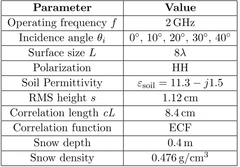
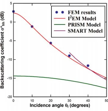
Figure 8 shows the results obtained of the co-polarized backscattering coefficient using the averaging process for a soil layer of permittivity εsoil = 11.3−j1.5 where the incident beam is H-polarized and

roughness conditions are as those found in Table 1. The co-polarized backscattering coefficient calculated using the FEM is compared with I2_{EM, PRSIM and SMART models. Results are in a good agreement}

with the I2EM model so that it can be applicable in our snow depth retrieval algorithm for the calculation of the backscattering contribution due the ground layer.

Figure 7. Three-layered structure setup in HFSS with the snow-ground interface being rough.

Table 1. Parameter values used in the HFSS simulation for a three-layered structure with a rough snow-ground interface.

Parameter Value

Operating frequencyf 2 GHz

Incidence angle θi 0◦, 10◦, 20◦, 30◦, 40◦

Surface size L 8λ

Polarization HH

Soil Permittivity εsoil= 11.3−j1.5

RMS heights 1.12 cm Correlation lengthcL 8.4 cm

Correlation function ECF

Snow depth 0.4 m

Figure 8. The backscattering coefficient as function of the incidence angle for the parameter values shown in Table 1 with a comparison with theoretical models.

3.4. Snow Density Estimation

The microwave response of snow covered ground is highly related to the snow grain size. At L-band, volume scattering contributions have no significant effect on the total received signal. That’s why snow is considered as a homogeneous mixture over a soil surface at L-band frequencies. In this case, the total backscattering coefficient σ_total0 at incident polarization p and received polarization q can be simplified to:

σ_total0 = T2_pq(θi)σ0g,pq(θr) (29)

where Tpq is the transmission from air to snow across the air-snow boundary, and σg is the surface

backscattering contribution from the snow-soil interface. For a horizontally polarized incident wave,Tpq

is defined as:

Th = 1−

cosθi−

ε_dscosθr

cosθi+

ε_dscosθr

2 (30)

where θi denotes the incidence angle andθr denotes the refraction angle in the snow layer. Snell’s law

states that:

sinθr= sinθi/√εds (31)

Note that the snow density is related empirically to the effective permittivity of snow by Looyenga’s semi-empirical dielectric formula as stated before. At L-band,σtotal is insensitive to snow depth as seen

theoretically in (8). That’s why in the numerical simulation in the section before, dcan be chosen to be any value.

The I2EM model is applied to simulate the ground surface backscattering coefficient (σg) under

snow cover. Ground (soil) surface parameters such as surface rms height s, correlation length cL, soil permittivity εsoil, and autocorrelation function (ACF) are used to compute the surface backscattering

value. For soil surfaces, the exponential correlation function (ECF) is a more realistic choice and it has been shown that ECF can be used to match active remote sensing experimental data [24].

The input variables used to findσtotal at L-band are: frequencyf, polarization pq, incidence angle

θi, snow density ρs or εds, dielectric constant of the ground εsoil, rms height of the ground surface

roughness s, ACF of the ground surface, correlation length of the ground surface roughnesscL.

Table 2. Parameter values used in the forward theoretical simulation at L-band.

Parameter Value

Operating frequencyf 2 GHz Incidence angle θi 0◦

Polarizationpq HH

Ground Permittivity 11.3−j1.5

RMS heights 0.6 cm

Correlation length cL 25 cm Autocorrelation function ECF

Snow density range study [0.25–0.5] g/cm3 Interval: 0.05

Table 3. Comparison between forward theoretical values and estimated values at L-band.

Snow density

(g/cm)3 εsnow theory εsnow retrieved ρs retrieved Density error in %

0.25 1.4291 1.4236 0.2472 1.12 %

0.3 1.5303 1.5311 0.3004 0.13 %

0.35 1.6399 1.6416 0.3509 0.26 %

0.4 1.7592 1.7632 0.4016 0.4 %

0.45 1.8773 1.8763 0.4496 0.09 %

0.5 1.9983 2.001 0.5011 0.22 %

formula. So, in our work, the parameters related to the ground surface are well known before snow fall. The values that were chosen in our forward theoretical simulation are summarized in Table 2. They are based on experimental data found in [4]. Then, the snow permittivity is solved using the non-linear Equations (29), (30), and (31). Then, the snow density is calculated using Equation (23).

Calculations are performed now using MATLAB where a zero-mean Gaussian noise with variance (σ2 = 0.02) is added to the theoretical values to form a statistical variation similar to that collected from a real radar. The study was done over a range of snow densities from 0.25 to 0.5 g/cm3 and a comparison is shown between simulated theoretical values and estimated values in Table 3. For each snow density, the HH-polarized backscattering coefficient is calculated and a Gaussian noise is added to the theoretical value to form a statistical variation as that in Figure 9(a). Then, the permittivity is solved for each value from the obtained histogram of the backscattering coefficient. Therefore, an estimate of the snow permittivity for a specific density is obtained by averaging the values of the new obtained histogram shown in Figure 9(b).

4. SNOW DEPTH RETRIEVAL ALGORITHM USING MULTIPLE OBSERVATIONS

The backscattering signals at X-band or higher frequency band is more sensitive to snow parameters so that the snow parameters inversion algorithm at these bands is more effective [25]. After the calculation of the snow density at L-band, the snow depth will be retrieved from backscattering measurements at X-band where volume scattering effects will have a significant effect on the total backscattering coefficient.

4.1. Volume Scattering Physical Model

(a) (b)

Figure 9. (a) Statistical distribution of the HH-polarized backscattering coefficient for air-snow-ground media for a snow density = 0.5 g/cm3 with parameter values found in Table 1. (b) Histogram of the retrieved permittivity of snow with density = 0.5 g/cm3 _{using the statistical distribution of the}

HH-polarized backscattering coefficient in Figure 9(a).

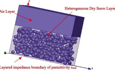
Figure 10. Three-layered structure setup in HFSS with planar interfaces and a heterogeneous snow volume.

ground layer covered by an inhomogeneous snow layer. So, the critical issue for this section is to test the validity of the volume backscattering effect through a careful numerical setup. The simulation setup for the calculation of the backscattering coefficient due to volume scatterers is shown in Figure 10. It consists of a dry snow layer of depthd= 0.1 m. This layer is treated as a heterogeneous mixture where uniformly distributed scatterers (ice crystals of r= 6 mm) are embedded in an air background.

just due to the heterogeneity structure of snow. But, the ground roughness will be not neglected when retrieving snow depth. It was ignored here for decreasing computation time because the verification of the validity of the I2_{EM model was done in the section before.}

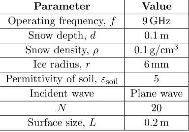
The procedure for calculating the bistatic scattering coefficient is the same as in Equation (9) where the averaging process is done for mixtures with the same volume fraction of ice but with different positioning of inclusions. Table 4 summarizes the values of the parameters used in the simulation setup.

Table 4. Parameter values used in the HFSS simulation for a three-layered structure with a heterogeneous snow medium.

Parameter Value Operating frequency,f 9 GHz Snow depth,d 0.1 m Snow density, ρ 0.1 g/cm3

Ice radius,r 6 mm Permittivity of soil, εsoil 5

Incident wave Plane wave

N 20

Surface size,L 0.2 m

The calculated numerical results of the co-polarized backscattering coefficient using the averaging process are shown in Figure 11 at different incidence angles with an H-polarized incident beam. A comparison was done withS2RT/R model where a good agreement is observed.

Figure 11. The calculated backscattering coefficient as a function of the incidence angle at H-polarization.

4.2. Snow Depth Retrieval Method

In our retrieval algorithm, the two chosen incidence angles were 10◦ and 30◦. These two incidence angles were chosen so that there is a much difference between their output values for parameter values shown in Figure 3. This is can be easily observed when calculating σg at 10 GHz for the obtained

snow density and soil surface parameters. Typically, in real measurements, a variety of incidence angles could be observed so that the collected experimental backscattered data could be all tested in the snow parameters retrieval. This algorithm performs best at 10◦ and 30◦ for such ground properties. Table 5 summarizes all the values chosen in the forward theoretical calculation at X-band.

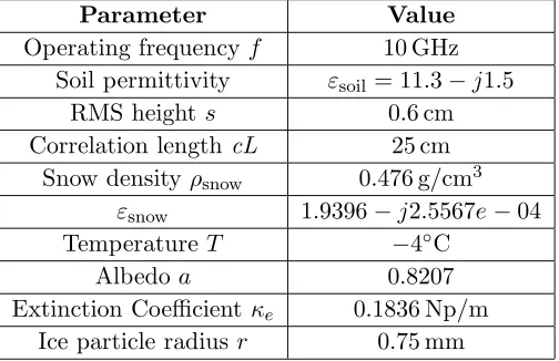
Table 5. Parameter values used in the forward theoretical simulation at X-band.

Parameter Value

Operating frequencyf 10 GHz Soil permittivity εsoil= 11.3−j1.5

RMS heights 0.6 cm Correlation length cL 25 cm

Snow density ρsnow 0.476 g/cm3

εsnow 1.9396−j2.5567e−04

TemperatureT −4◦C

Albedoa 0.8207

Extinction Coefficient κe 0.1836 Np/m

Ice particle radius r 0.75 mm

To retrieve snow depth, the density is calculated first using the previous procedure. Knowing the density, the refraction angle θr can be easily calculated from Snell’s law and then Tpq, Υpq, and Γg can

be computed. After replacing κs witha×κe, the remaining unknowns in Equation (3) are: the albedo

(a) and the snow optical depth (τ) which is the product of the extinction coefficient (κe) and the snow

depth (d):

τ =κed (32)

The extinction coefficient is related to the albedo by:

κe =κa/(1−a) (33)

where the volume absorption coefficient is defined empirically by:

κa=vik0

ε_ice εair

3εair

εice+ 2εair

2 (34)

whereε_iceis the imaginary part of the permittivity of ice, and it is determined from snow temperature. The retrieval process can be summarized as follows:

(i) Using dual incidence angles, the albedo and the snow optical thickness can be calculated using the non-linear relationship between the backscatter values and the snow parameters in Equation (3). (ii) Calculate κa using Equation (34).

(iii) Calculate κe using Equation (33) with the estimated value of the albedo in step 1.

(iv) Finally, snow depth can be easily retrieved using (32).

The HH-polarized backscattering coefficient is calculated for each snow depth value for two incidence angles, and a Gaussian noise is added to the theoretical value forming a statistical variation ofσtotalas shown in Figure 12. Then, the albedo (a) and the snow optical depth (τ) are solved for each

value from the obtained two histograms of σtotal. So, another two histograms will be obtained for a

Figure 12. Statistical distribution of theHH-polarized backscattering coefficient from air-snow-ground for a snow density = 0.476 g/cm3 and snow depth = 1 m with parameter values found in Table 5 at θi= 10 (Blue) and θi= 30 (Red).

Table 6. Comparison between forward theoretical values and estimated values at X-band.

d (cm) albedo ‘a’ d-retrieved (cm) a-retrieved Error in d (%)

50 0.8207 48.91 0.8426 2.18

75 0.8207 74.59 0.8416 0.546

100 0.8207 100.61 0.8303 0.61

125 0.8207 125.30 0.8317 0.24

150 0.8207 150.97 0.8255 0.646

175 0.8207 176.45 0.8272 0.828

200 0.8207 203.59 0.8224 1.795

225 0.8207 223.46 0.8364 0.684

250 0.8207 248.34 0.8393 0.664

275 0.8207 276.42 0.8336 0.516

300 0.8207 302.56 0.8361 0.853

4.3. Sensitivity of Snow Thickness Estimates to Errors in Snow Density

Provided with a 10 GHz operating radar, the measured backscattering coefficient depends mainly on the snow density. Knowledge of the effective permittivity of snow is essential to accurately derive the snow layer thickness, hence it is necessary to measure the sensitivity of the radar to errors in estimates of the snow density. Table 7 shows that there is an increasing error made in distance calculations as the error in the density estimation increases. The values in Table 7 show that for a dry snow pack a 20% error in density contributes approximately a 13.85% error to snow thickness (for example, if the snow thickness is 100 cm, this is gives a 13.85 cm error in snow thickness).

Table 7. Error in snow pack thickness calculations as a function of error in density for dry snow.

ρs = 0.3 g/cm3 ρs ρs+10% ρs-10% ρs+20% ρs−20 %

Figure 13. Comparison of the estimated snow depth using the previous algorithm with a 0.02 noise variance with real input data.

5. CONCLUSION

In this paper, forward theoretical physical models regarding the propagation properties of snow were tested numerically in an electromagnetic simulator. The choice of Looyenga’s model in density estimation and the I2EM model for surface scattering calculations were the best. Then, a snow depth retrieval algorithm was proposed based on backscattering measurements at L- and X-band using multi-incidence angles. This algorithm requires a priori knowledge of the dielectric and roughness properties of the ground. Estimated values were in an excellent agreement with simulated ones showing an error of less than 2% for a 0.02 noise variance. Our future work is to validate this algorithm experimentally with the use of a MIMO radar.

ACKNOWLEDGMENT

This work is supported by the Lebanese University (UL).

REFERENCES

1. Barnett, T. P., J. C. Adam, and D. P. Lettenmaier, “Potential impacts of a warming climate on water availability in snow-dominated region,” Nature, Vol. 438, No. 7066, 303–309, 2005.

2. Cui, Y., C. Xiong, J. Lemmetyinen, J. Shi, L. Jiang, B. Peng, H. Li, T. Zhao, D. Ji, and A. T. Hu, “Estimating Snow Water Equivalent with backscattering at X and Ku band based on absorption loss,” Remote Sensing, Vol. 8, No. 6, 505, 2016.

3. Shi, J. and A. J. Dozier, “Estimation of snow water equivalence using SIR-C/X-SAR. I. Inferring snow density and subsurface properties,” IEEE Transactions on Geoscience and Remote Sensing, Vol. 38, No. 6, 2465–2474, 2000.

4. Ulaby, F. T., D. G. Long, W. J. Blackwell, C. Elachi, A. K. Fung, C. Ruf, K. Sarabandi, H. A. Zebker, and J. Van Zyl, Microwave Radar and Radiometric Remote Sensing, Vol. 4, University of Michigan Press Ann Arbor, 2014.

6. Shi, J., “Snow water equivalence retrieval using X and Ku band dual-polarization radar,” IEEE International Conference on Geoscience and Remote Sensing Symposium, 2006. IGARSS 2006, 2183–2185, IEEE, July 2006.

7. http://www.ansoft.com/produxts/hf/hfss/.

8. Oh, Y., K. Sarabandi, and F. T. Ulaby, “An empirical model and an inversion technique for radar scattering from bare soil surfaces,”IEEE transactions on Geoscience and Remote Sensing, Vol. 30, No. 2, 370–381, 1992.

9. Dubois, P. C., J. Van Zyl, and T. Engman, “Measuring soil moisture with imaging radars,” IEEE Transactions on Geoscience and Remote Sensing, Vol. 33, No. 4, 915–926, 1995.

10. Ghafouri, A., J. Amini, M. Dehmollaian, and M. A. Kavoosi, “Better estimated iem input parameters using random fractal geometry applied on multi-frequency SAR data,”Remote Sensing, Vol. 9, No. 5, 445, 2017.

11. Fung, A. K., K. S. Chen, and K. S. Chen,Microwave Scattering and Emission Models for Users, Artech House, 2010.

12. Hopsø, I. S., Wet Snow Detection by C-band SAR in Avalanche Forecasting, Master’s thesis, UiT The Arctic University of Norway, 2013.

13. Fayad, A., S. Gascoin, G. Faour, P. Fanise, L. Drapeau, J. Somma, and R. Escadafal, “Snow observations in Mount Lebanon 2011–2016,” Earth System Science Data, Vol. 9, No. 2, 573, 2017. 14. Sihvola, A. H. and J. A. Kong, “Effective permittivity of dielectric mixtures,”IEEE Transactions

on Geoscience and Remote Sensing, Vol. 26, No. 4, 420–429, 1988.

15. Matzler, C. and U. Wegmuller, “Dielectric properties of freshwater ice at microwave frequencies,”

Journal of Physics D: Applied Physics, Vol. 20, No. 12, 1623, 1987.

16. Hallikainen, M., F. Ulaby, and M. Abdelrazik, “Dielectric properties of snow in the 3 to 37 GHz range,”IEEE transactions on Antennas and Propagation, Vol. 34, No. 11, 1329–1340, 1986. 17. Looyenga, H., “Dielectric constants of heterogeneous mixtures,” Physica, Vol. 31, No. 3, 401–406,

1965.

18. Qi, J., H. Kettunen, H. Wall´en, and A. Sihvola, “Different retrieval methods based onS-parameters for the permittivity of composites,” 2010 URSI International Symposium on Electromagnetic Theory (EMTS), 588–591, IEEE, August 2010.

19. Jin, Y. Q. and Z. Li, “Simulation of scattering from complex rough surfaces at low grazing angle incidence using the GFBM/SAA method,” IEEJ Transactions on Fundamentals and Materials, Vol. 121, No. 10, 917–921, 2001.

20. Ye, H. and Y. Q. Jin, “Parameterization of the tapered incident wave for numerical simulation of electromagnetic scattering from rough surface,”IEEE Transactions on Antennas and Propagation, Vol. 53, No. 3, 1234–1237, 2005.

21. Tsang, L., J. A. Kong, and K. H. Ding, Scattering of Electromagnetic Waves: Theories and Applications, John Wisley and Sons, 2000.

22. Lawrence, H., F. Demontoux, J. P. Wigneron, A. Mialon, T. D. Wu, V. Mironov, and Y. Kerr, “L-band emission of rough surfaces: Comparison between experimental data and different modeling approaches,” 2010 11th Specialist Meeting on Microwave Radiometry and Remote Sensing of the Environment (MicroRad), 27–32, IEEE, March 2010.

23. Fung, A. K., M. R. Shah, and S. Tjuatja, “Numerical simulation of scattering from three-dimensional randomly rough surfaces,” IEEE Transactions on Geoscience and Remote Sensing, Vol. 32, No. 5, 986–994, 1994.

24. Zhou, L., L. Tsang, V. Jandhyala, Q. Li, and C. H. Chan, “Emissivity simulations in passive microwave remote sensing with 3-D numerical solutions of Maxwell equations,” IEEE transactions on Geoscience and Remote Sensing, Vol. 42, No. 8, 1739–1748, 2004.

25. Shi, J., C. Xiong, and L. Jiang, “Review of snow water equivalent microwave remote sensing,”

Multiple Backscattering Measurements for Snow Depth Retrieval”

by Fatima Mazeh, Bilal Hammoud, Hussam Ayad, Fabien Ndagijimana,

Ghaleb Faour, Majida Fadlallah, and Jalal Jomaah

in Progress In Electromagnetics Research B, Vol. 81, 63–80, 2018

Fatima Mazeh1, 2, *, Bilal Hammoud1, 2, 3, Hussam Ayad1, Fabien Ndagijimana2, Ghaleb Faour3, Majida Fadlallah1, and Jalal Jomaah1

ACKNOWLEDGMENT

This work is supported by the Lebanese University (UL) and partially funded by the National Council for Scientific Research (CNRS) in Lebanon.

Received 15 October 2019, Added 17 October 2019

* Corresponding author: Fatima Mazeh ([email protected]).

1 _{Physics Department, Faculty of Sciences, Lebanese University, Beirut, Lebanon.} 2 _{Grenoble University, Grenoble, France.} 3