Local Search Approximation Algorithms for Clustering Problems

(1)

Scholarship@Western

Electronic Thesis and Dissertation Repository

4-5-2019 3:30 PM

Local Search Approximation Algorithms for Clustering Problems

Nasim Samei

The University of Western Ontario

Supervisor

Professor Roberto Solis-Oba The University of Western Ontario Graduate Program in Computer Science

A thesis submitted in partial fulfillment of the requirements for the degree in Doctor of Philosophy

Follow this and additional works at: https://ir.lib.uwo.ca/etd

Part of the Theory and Algorithms Commons

Recommended Citation Recommended Citation

Samei, Nasim, "Local Search Approximation Algorithms for Clustering Problems" (2019). Electronic Thesis and Dissertation Repository. 6138.

https://ir.lib.uwo.ca/etd/6138

This Dissertation/Thesis is brought to you for free and open access by Scholarship@Western. It has been accepted for inclusion in Electronic Thesis and Dissertation Repository by an authorized administrator of

(2)

In this research we study the use of local search in the design of approximation algorithms for NP-hard optimization problems. For our study we have selected several important and well known clustering problems: k-uncapacitated facility location problem, minimum mutliway cut problem, and constrained maximum k-cut problem.

We show that by careful use of the local optimality property of the solutions produced by local search algorithms it is possible to bound the ratio between solutions produced by local search approximation algorithms and optimum solutions. This ratio is what is known as the locality gap of the algorithms.

The locality gap of our algorithm for the k-uncapacitated facility location problem is 2 +√3 + for any constant > 0. This matches the approximation ratio of the best known algorithm for the problem, proposed by Zhang but our algorithm is simpler. For the minimum multiway cut problem our algorithm has locality gap 2-2/k, which matches the approximation ratio of the isolation heuristic of Dahlhaus et al; however, our experimental results show that in practice our local search algorithm greatly outperforms the isolation heuristic, and furthermore it has comparable performance as that of the three currently best algorithms for the minimum multiway cut problem (by Calinescu et al, Sharma and Vondrak, and Buchbinder et al). For the constrained maximum k-cut problem on hypergraphs we proposed a local search based approximation algorithm with locality gap 1-1/k for a variety of constraints imposed on thek-cuts. The locality gap of our algorithm matches the approximation ratio of the best known algorithm for the max k-cut problem on graphs designed by Vazirani, but our algorithm is more general.

Keywords: Combinatorial optimization, Approximation algorithms, Local search,

Facility location problem, Multiway cut problem, Max k-cut problem

(3)

This thesis consists of three research articles that either have already been published or that are currently being considered for publication in specialized journals. The contri-butions of each one of the authors are listed below. Authors are listed in alphabetical order.

Chapter 2 includes an article titled ”Analysis of a local search algorithm for the k-facility location problem” published in the journal RAIRO-Theoretical Informatics and Applications. Nasim Samei provided some research ideas, she contributed to the analysis of the algorithms and wrote the first draft of the paper. Roberto Solis-Oba contributed with research ideas leading to the design of the algorithm and analysis of the algorithms; he also edited the manuscript.

Chapter 3 includes an article titled ”A local search algorithm for the multiway cut problem” submitted to Journal of Computer and System Sciences. Andrew Bloch-Hansen implemented the algorithms and performed the experiments; he also wrote the part of the manuscript describing the experimental results. Nasim Samei contributed with research ideas that let to the design of the algorithms and their analysis. She wrote the first draft of the paper. Roberto Solis-Oba contributed with ideas about design and analysis of the algorithm, he also edited the manuscript.

Chapter 4 includes an article titled ”A local search algorithm for the constrained maxk-cut problem on hypergraphs” that is currently under review in Journal of Applied Mathematics and Computing. Nasim Samei contributed with research ideas that let to the design of the algorithms and their analysis. She wrote the first draft of the paper. Roberto Solis-Oba contributed with ideas about design and analysis of the algorithm, he also edited the manuscript.

(4)

I would like to express my sincere gratitude to my supervisor, Roberto Solis-Oba, for having strong faith in me. Also, I am very thankful for all his tremendous support in all aspects of my professional development. He is a great mentor and knowledgeable supervisor who provided me with wise advice. This thesis would not be possible without his extraordinary perseverance. I am forever indebted to him.

I am grateful to my examining committee, Yuri Boykov, Hamada Ghenniwa, Daniel Lizotte and Marc Moreno Maza for accepting to be my examiners and their constructive feedback.

I am privileged to have a supportive and understanding family. My greatest thanks to my parents Nastaran and Rasoul for their fantastic support throughout my Ph.D. program especially their great support and patience on my Ph.D. exam date. Also, I am thankful for their great respect for my choices and providing me an environment that I can learn and grow.

(5)

Abstract

List of Figures vi

List of Tables viii

1 An Introduction to Combinatorial Optimization Problems 1

1.1 Introduction . . . 1

1.2 Local Search Algorithms . . . 5

1.3 The Complexity of Computing Local Optimum Solutions . . . 10

1.4 Local Search in the Design of Approximation Algorithms . . . 11

1.5 Local Search for Combinatorial Optimization Problems . . . 13

1.5.1 The Multiprocessor Scheduling Problem . . . 13

1.5.2 Computing a Spanning Tree with Many Leaves . . . 14

1.5.3 The k-Set Packing Problem . . . 14

1.5.4 The Max k-SAT Problem . . . 15

1.5.5 The Traveling Salesman Problem . . . 15

1.5.6 The Quadratic Assignment Problem . . . 16

1.5.7 The k-Set Cover Problem . . . 17

1.5.8 The Maximum Constraint Satisfaction Problem . . . 17

1.5.9 The Stable Marriage Problem . . . 18

1.5.10 Placement of Meters in Networks . . . 19

1.6 Our Local Search Algorithms . . . 19

1.6.1 The k-Facility Location Problem . . . 19

1.6.2 The Multiway Cut Problem . . . 20

1.6.3 The Constrained Max k-cut Problem on Hypergraphs . . . 22

1.7 Organization of the Thesis . . . 25

Bibliography 26 2 Local Search Algorithm for the k-Facility Location Problem 28 2.1 Introduction . . . 28

2.1.1 Contributions . . . 29

2.1.2 Organization of the Paper . . . 29

2.2 A Local Search Algorithm with Multiple Swaps . . . 30

2.3 First Bound for the Locality Gap . . . 32

(6)

Multi-Swaps for SetsAi and Bi where |Ai|=|Bi|≤p . . . 35

Swaps for Sets Ai and Bi where|Ai|=|Bi|> p . . . 36

Single Swaps for Facilities in Sets Ar and Br . . . 40

Putting It All Together . . . 40

2.3.3 Special Case When the Ratio of the Biggest Facility Cost to the Smallest Facility Cost Is Less Thanp+ 1 . . . 41

2.4 Tight Example . . . 42

2.5 Scaling the Costs . . . 43

2.5.1 Bounding the Facility Cost . . . 44

2.5.2 Bounding the Service Cost . . . 45

Bibliography 48 3 A Local Search Algorithm for the Multiway Cut Problem 50 3.1 Introduction . . . 50

3.2 The Local Search Algorithm . . . 51

3.3 Finding a minimum cost relabel operation . . . 53

3.4 Algorithm MULTIWAY CUT for the 3-way Cut Problem . . . 56

3.4.1 First bound . . . 58

3.4.2 Second Bound . . . 61

3.4.3 Computing the Approximation Ratio . . . 62

3.5 The Multiway Cut Problem . . . 62

3.5.1 First Bound . . . 63

3.5.2 Second bound . . . 65

3.5.3 Computing the Approximation Ratio . . . 66

3.6 Tight Example . . . 67

3.7 Variations of the Multiway Cut Problem . . . 68

3.7.1 Nodes that Need to be in the Same Partition . . . 68

3.7.2 Nodes that Can Only be in Some Partitions . . . 70

3.8 Experimental Results . . . 71

3.8.1 Input Data . . . 71

3.8.2 Test Cases . . . 72

3.8.3 Results . . . 73

Input Networks . . . 74

Graph Characteristics . . . 75

Running Time . . . 78

Initial Labeling and Value of . . . 79

3.8.4 Final Observations . . . 81

3.8.5 Acknowledgements . . . 81

Bibliography 82

4 Local Search for the Constrained Max k-Cut Problem 84

(7)

4.3 Max k-Cut, Max Multiway Cut, and Max Steiner k-Cut Problems . . . . 88 4.4 Max Capacitatedk-Cut, Max k-Cut with Given Sizes of Parts . . . 90 4.5 Directed Max k-Cut Problem . . . 93

Bibliography 99

5 Conclusions 101

5.1 Main Contributions . . . 101 5.2 Challenges of Using Local Search in the Design of Approximation Algorithms102 5.3 Strengths of Local Search Algorithms . . . 103

Bibliography 104

Curriculum Vitae 104

(8)

1.1 An instance of the traveling salesman problem. . . 1 1.2 Example of the single swap operation and the corresponding neighborhood

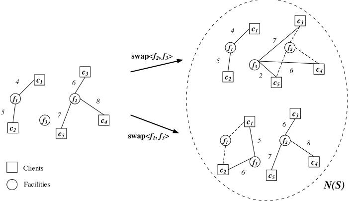
function, where F = {f1, f2, f3} and C = {c1, c2, c3, c4, c5}. Clients are

connected with solid lines to the facilities that service them, and a client is connected to a facility with a dashed line if that facility was servicing the client before performing the swap but it does not service the client after the swap. . . 6 1.3 Example of a local optimal solution and a global optimal solution for an

instance of the facility location problem. . . 7 1.4 Example of a scheduling problem. . . 8 1.5 Initial solution for the minimum multiway cut. . . 9 1.6 Local optimal solution and global optimal solution for the example of the

multiway cut problem in Figure 1.5. . . 10 1.7 Instance illustrating a big locality gap for a scheduling problem using the

jump operation. . . 12 1.8 An example of the 2-opt neighborhood. . . 16 1.9 Example of a multi-swap operation, whereS ={s1, s2, s3},A={s1, s2, s3}

and B ={f1, f2, f3}. . . 20

1.10 Instance of the multiway cut problem, where k = 4 andT ={t1, t2, t3, t4};

one possible solution for this instance of the problem is to divide the vertices into partitions V1, V2, V3, V4 and the cost of this solution is 14. . . 21

1.11 Instance of the labelling version of the multiway cut problem. . . 21 1.12 Example of a relabel operation RhA, α, fi, where A={p, q} and α =l3. . 22

1.13 Instance of the max k-cut problem. . . 23 1.14 Instance of the max k-cut problem on hypergraphs. . . 23 1.15 Example of local operations. The dashed edges in Figures (a1) and (b1)

are the edges that are added to the cost of the solution after performing the corresponding local operation. The dashed edges in Figures (a2) and

(b2) are the edges that no longer contribute to the cost of the solution after

performing the local operation. . . 24 2.1 Mappingπ maps eacho ∈S∗ to its closest facility π(o)∈S. . . 32 2.2 Clientj ∈NS(Ai)\NS∗(Bi) is assigned to ˆs=π(σ∗(j)). Note that σ∗(j)6∈

Bi and π(σ∗(j))6∈Ai. . . 36

2.3 Tight example for p= 2 and q= 5. . . 43 2.4 Tight example for arbitraryp and q. . . 43

(9)

are represented by circles. InGlabels assigned to the nodes are inside the squares. . . 53 3.2 PathsP and P0 are shown above in thick and thin solid lines, respectively. 54 3.3 The left figure shows partitions Â1, Â2 and Â3 of the local optimal solution

and the right figure shows partitions A∗₁, A∗₂ and A∗₃ of the global optimal solution. In both figures the set of edges that contribute to the 3-way cut connect nodes in different partitions. For example, edge (u, v) in the left figure connects u∈Aˆ1 tov ∈Aˆ2 so it contributes to the cost of the local

optimal solution, and edge (u, w) in the right figure connects u ∈ A∗₁ to

w∈A∗₂ so it contributes to the cost of the global optimal solution. . . 57 3.4 In all the figures, partitions ( ˆA1,Aˆ2,Aˆ3) and (A∗1, A

∗

2, A

∗

3) are as in Figure

3.3. Figure (a) represents the set ∆1, Figure (b) represents set ∆2, and

Figure (c) represents set ∆. . . 59 3.5 Node labels are inside the nodes and node names are written beside the

nodes. Edge costs are written beside the edges. The terminals arex1, x2, . . . , xk. 68

3.6 An example of the transformation ofG intoG0. Nodes that need to be in the same partition ares, q, u, pso in the transformed graphG0 a super node

Q is created for these nodes. Also, cost(t1, Q) = cost(u, t1) +cost(t1, p)

and cost(Q, r) = cost(p, r). . . 69 3.7 Results from the 80 vertex exponential decay graph distribution: Average

approximation ratios with 5 terminals (top-left), maximum approximation ratios with 5 terminals (top-right), average approximation ratios with 5n

edge density (bottom-left), maximum approximation ratios with 5n edge density (bottom-right). . . 77 3.8 Results from the 160 vertex exponential decay graph distribution with

m = 4n and k = 10. Approximation ratios are compared against the epsilon value using the first edge capacity scheme (top-left) and the second edge capacity scheme (bottom-left). Running times are compared against the epsilon value using the first edge capacity scheme (top-right) and the second edge capacity scheme (bottom-right). The x-axis shows the value of

/k2_{; the percentage of improvement to the previous best solution required}

to continue the iterations of the algorithm. . . 80 4.1 Example of a directed Hypergraph. . . 93

(10)

3.1 Weights for the edges inGα. . . 54

3.2 Ratios of the solutions computed by approximation algorithms to the op-timum, for benchmarks from the DIMACS competitions: Maximum inde-pendent set (Brock), maximum clique (Gen, C125), Hamming instances, Keller instances, p-hat instances, and Steiner tree instances (ST). Ratios for the randomly generated instances with simple (SR), linear (GL), and exponential (GE) distributions. . . 75 3.3 Average and maximum approximation ratios for several test cases on 80

vertex random graphs with exponential decay distributions. . . 76 3.4 Running times using 100 experiments for several test cases from the 80

vertex and 160 vertex exponential decay distributions. . . 78

(11)

An Introduction to Combinatorial

Optimization Problems and Local

Search

1.1 Introduction

In a combinatorial optimization problem we look for a that either maximizes or mini-mizes a given objective function. A feasible solution usually requires grouping, ordering or selecting a discrete or finite set of objects that satisfies some given conditions; there-fore the solution space (the set of all feasible solutions) for a combinatorial optimization problem is discrete or finite. Usually the solution spaces of combinatorial optimization problems are very large and thus using exhaustive search to find optimal solutions, solu-tions that either maximize or minimize an objective function, is not efficient. Therefore, it is of great interest to design more sophisticated algorithms that can find optimal or near optimal solutions in polynomial time.

A classical example of a combinatorial optimization problem is the traveling salesman problem in which we are given a weighted graph G = (V, E) and the goal is to find a minimum weightHamiltonian cycle. A Hamiltonian cycle is a cycle that includes all the nodes of G.

1

3 4

2 35

20

30 25

Figure 1.1: An instance of the traveling salesman problem.

Figure 1.1 shows an instance of the traveling salesman problem; the solution space includes all possible Hamiltonian cycles: (2, 1, 4, 3, 2), (2, 1, 3, 4, 2), (2, 4, 1, 3, 2), (2,

(12)

4, 3, 1, 2), (2, 3, 1, 4, 2) and (2, 3, 4, 1, 2). The weights of these cycles (the objective function) are: 95, 80, 95, 80, 95 and 95, respectively. A feasible solution is any cycle from the solution space. An optimal solution is any cycle with the smallest weight. In this example cycles (2, 1, 3, 4, 2) and (2, 4, 3, 1, 2) are optimal. Observe that in this example since the size of the solution space is small we can quickly find an optimal solution, however for larger instances the solution space would be huge and it would be very difficult to find optimum solutions.

Combinatorial optimization problems are of great importance because many real life problems can be modeled as combinatorial optimization problems. These problems arise in a wide variety of fields, such as data mining, information retrieval, network routing, image processing, machine learning, artificial intelligence, operation research, and so on. In addition, combinatorial optimization is of great theoretical importance because it led to advances in other areas such as discrete mathematics, computer science, probability theory, and continuous optimization.

Many important combinatorial optimization problems are NP-hard [2]; this means that there is very strong theoretical evidence suggesting that there are no polynomial time algorithms for solving them. An effective approach for dealing with NP-hard problems is to find solutions that are provably close to the optimal solutions. Algorithms that find these near optimal solutions are called approximation algorithms. To measure the quality of an approximation algorithm we compute itsapproximation ratio. If an algorithm has approximation ratio α then the solutions returned by the algorithm are guaranteed to have values that are within an α factor of the optimal solutions.

We are interested in studying and designing approximation algorithms because, as mentioned earlier, in real life we need to solve NP-hard problems. The analysis of ap-proximation algorithms helps us understand why some approaches work better on some problems and hence it gives us clues on which approaches would be more promising for a new problem. Moreover, approximation algorithms give us a metric on how ”hard” different NP-hard problems are.

Due to their importance, there is extensive research in the literature on the design of approximation algorithms. These algorithms have been designed for problems from a large variety of fields and several methodologies have shown to be effective for the design and analysis of approximation algorithms.

We can classify approaches for designing approximation algorithms into two main categories; non-linear programming based approaches and linear programming based approaches. We describe below several non-linear programming-based approaches.

• Greedy algorithms: Greedy algorithms usually start with an empty solution and

they repeatedly make ”greedy” choices that select a ”locally” optimal way to enlarge the current solution in the hope that at the end they will find an optimal solution. In these algorithms once a decision is made the decision cannot be modified. Greedy algorithms are usually very fast and they are easy to implement. However, they do not always produce near optimal solutions.

• Local search algorithms: A local search algorithm starts with an arbitrary

(13)

neighbor solution with a better objective function value. The algorithm stops when no further improvement is possible. The neighbors of a given feasible solution are determined by a set of local operations. A local operation transforms a given solu-tion s into a new feasible solutions0 by usually performing simple changes such as adding, removing or swapping elements ofswith some other elements not ins(later we give more examples of local operations). The main reason we are interested in local search is that local search algorithms are conceptually simple and they are usually easy to implement. We believe that local search is a powerful technique that can be used to design efficient approximation algorithms, but so far there are relatively few research works published on the design of local search approximation algorithms. In this thesis we explore the use of local search in the design of algo-rithms for NP-hard optimization problems with a provable performance guarantee. We will discuss this class of algorithms in more detail in the next section.

• Dynamic programming: A dynamic program decomposes a problem into smaller

sub-problems that have smaller solution spaces than the original one. The solutions to the smaller problems are combined to construct solutions for bigger sub-problems until we obtain a solution for the entire problem. The main advantages of dynamic programming are: (1) we limit the size of the solution space by breaking down the problem into smaller sub-problems, and (2) in the process of recursively breaking down the problem into simpler sub-problems and considering different ways of combining the solutions of these sub-problems to form a global solution, we might encounter the same sub-problems many times, but they need to be solved only once.

Now, we give a brief introduction to integer and linear programming and linear pro-gramming based approaches for the design of approximation algorithms. In an integer program we are given a set ofvariables that can only take integer values and that need to satisfy some constrains specified in the form of linear inequalities or linear equations. A

feasible solution is an assignment of values to the variables that satisfies the constraints. The goal is to find a feasible solution that optimizes a given objective function; the objec-tive function is a linear combination of the variables. An integer minimization program is usually expressed in matrix form as follows,

min cTx

s.t. Ax ≤ b x integer

(1.1)

where x is a vector containing the variables and c is a vector of cost coefficients; vector

b and coefficient matrix A define the constraints of the integer program. Observe that a maximization integer program can be converted to a minimization integer program by simply multiplying each cost coefficient by -1.

(14)

be solved in polynomial time, but the solution of a linear program is not guaranteed to assign integer values to the variables; hence solving a linear program does not in general give a feasible solution to a combinatorial optimization problem formulated as an integer program. Each solution of the linear program relaxation of an integer program is called a fractional solution.

There are several linear programming based techniques for designing approximation algorithms; these techniques differ in how fractional solutions are manipulated to produce integer solutions. Some of these techniques are briefly described below.

• Deterministic rounding: As mentioned above solving the linear programming

relaxation of a combinatorial optimization problem gives a solution that assigns fractional values to the variables, however we are interested in a solution with integer values on the variables. Rounding methods convert a fractional solution to a feasible solution for a combinatorial optimization problem, by rounding up or down the values of the variables to integer values. The rounding must be done in such a way that the value of the rounded solution is close to the value of the fractional one as this ensures that the obtained solution has value close to the optimal.

• Rounding a dual solution: In this method a feasible solution to an optimization

problem is obtained by rounding the dual of the linear program relaxation of an optimization problem. Each linear program P has associated another linear pro-gram P0, called its dual. Linear program P is called primal. Optimal solutions for primal and dual linear programs have the same value. Furthermore, if P is a maximization linear program P0 is a minimization linear program and vice versa. The number of constraints in the primal is equal to the number of variables in the dual and the number of variables in the primal is equal to the number of constraints in the dual. Sometimes, solving the primal linear program is difficult but it is easy to find a solution for the dual, for instance when there are too many variables in the primal. When this happens we solve the dual of the linear program and then we round it to find an approximate solution for the optimization problem.

• The primal-dual method: In this method instead of solving the dual of the

linear program, we simultaneously build solutions for the linear program and its dual. We start with a feasible but expensive solution for the dual problem and an infeasible solution for the primal. Then we gradually improve the cost of the dual solution while at the same time reducing the number of constraints not satisfied by the primal solution. At the end we get a feasible solution for the primal and a near optimal solution for the dual. By the properties of the primal and dual linear programs, the primal solution also has value close to the optimal.

• Randomized rounding: In this method we solve the linear program relaxation

(15)

approximation algorithms for difficult problems that cannot be solved using other techniques.

Even though linear programming based approximation algorithms have beed successfully designed for a large number of NP-hard optimization problems, one of the main drawbacks of these algorithms is their big running times due to the fact that they have to solve linear programs. The focus of this thesis is on the use of local search in the design of approximation algorithms. As we show this technique can be used to design efficient algorithms with good approximation ratios.

1.2 Local Search Algorithms

As we mentioned earlier, in combinatorial optimization we look for a solution S from the solution space A, that optimizes an objective function c: A −→ _Q, where _Q is the set of rational numbers. A local search algorithm is defined by its local operations. A local operation op(S) transforms a solutionS ∈ Ainto a new solutionS0 by for example, adding, removing or exchanging elements ofS with elements not inS. Local operations are usually simple and they should be able to be performed quickly with algorithms with low running times. A neighborhood function N is defined by the local operations. For each solution S ∈ A, N(S) includes all the solutions S0 ∈ A that can be obtained by performing a local operation on S.

The facility location problem is a central problem in combinatorial optimization. In this problem we are given a set F of facilities, a set C of clients, service costs c, and opening facility costs f. Let cij be the cost of serving client i by facilityj and let fj be

the opening cost for facility j. The goal is to select a set S of facilities and to assign clients to facilities in such a way that minimizes the service cost plus the cost of opening the facilities needed to service the clients. Therefore, we want to minimize the following cost function,

cost(S) = Σi∈Sfi+ Σj∈Ccjσ(j), (1.2)

whereS is a set of facilities and σ(j) is the facility inS with the smallest service cost to client j. One possible local operation applicable to the facility location problem is the

(16)

f1 f3

f2

c1

c2

c3

c5

c4 2

4

5

6

7

8

f1 f3

f2

c1

c2

c3

c5

c4 2

4

5

6 7

f1 f3

f2

c1

c2

c3

c5

c4

2 ₆

5 6

7

8 2

swap<f2, f3>

swap<f1, f3>

N(S)

Clients

Facilities

Figure 1.2: Example of the single swap operation and the corresponding neighborhood function, where F = {f1, f2, f3} and C = {c1, c2, c3, c4, c5}. Clients are connected with

solid lines to the facilities that service them, and a client is connected to a facility with a dashed line if that facility was servicing the client before performing the swap but it does not service the client after the swap.

Consider the example shown in Figure 1.2; assume all the facility opening costs are 0, then the cost of the solution S ={f1, f2}is equal to the sum of the clients service costs,

which is 30. Figure 1.2 shows two neighbouring solutions of S obtained by performing

swap < f2, f3 >and swap < f1, f3 >. By performing swap < f2, f3 >the cost improves

to 24 and by doing swap < f1, f3 >the cost increases to 32.

There are several variants of local search algorithms. In this thesis we focus on

iter-ative improvement local search algorithms, formally described below. Note that a local

optimum solution might not be a global optimal solution as we show in the examples presented later. The locality gap of a local search algorithm is the largest ratio of the value of a local optimal solution produced by the algorithm to the value of a correspond-ing global optimal solution. LetsI be a local optimal solution produced by a local search algorithm for some instance I of a maximization problem P and let s∗(I) be a global optimal solution for I, then the locality gap of the algorithm is defined as minI∈P c(s(

I)) c(s∗₍_I₎₎,

where c(s(I)) is the cost of s(I) and c(s∗(I)) is the cost of s∗(I). Similarly, for mini-mization problemsP the locality gap is defined as maxI∈P

(17)

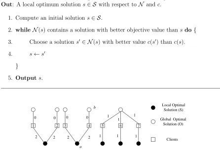
Algorithm IterativeImprovement(S,N, c)

In: Set S of feasible solutions, neighborhood function N and objective function c.

Out: A local optimum solution s ∈ S with respect toN and c. 1. Compute an initial solution s∈ S.

2. while N(s) contains a solution with better objective value than s do {

3. Choose a solution s0 ∈ N(s) with better value c(s0) than c(s). 4. s ←s0

}

5. Output s.

1 2 3 4 5 6 7

Clients Global Optimal

Solution (O) Local Optimal

Solution (S)

2 2 2 2

0 0 0 0 1

1 1 1

1 1

b

a

Figure 1.3: Example of a local optimal solution and a global optimal solution for an instance of the facility location problem.

Figure 1.3 shows an instance of the facility location problem with 10 facilities and 7 clients. A local optimal solution S consists of the facilities represented by the black circles and the global optimal solution O contains the facilities represented with white circles; cost(S) is 11 and cost(O) is 3. Observe that S is a local optimal solution with respect to the single swap operation because no single swap operation can improve its cost: For example if we performswap<a,b> then clients 3 and 4 are serviced by facilityb

at costs 0 and 4 respectively, so the total cost remains unchanged. Observe thatS is the worst local optimal solution because no other selection of 5 facilities has a worse cost. Therefore, the local search algorithm with single swap as the local operation has locality gap 11₃ for this instance of the facility location problem.

We present two more examples to illustrate how a local search algorithm gradually improves an initial solution to obtain a final solution with the property that no further improvement is possible.

We start by considering a scheduling problem in which we are given a set J ofn jobs

J ={j1, j2, ..., jn}, a set of m processors M ={M1, M2, ..., Mm}, and processing time pi

for each job ji, i= 1,2, ..n. The goal is to schedule jobs on processors so as to minimize

(18)

the processing of a job cannot be interrupted, i.e. preemptions are not allowed.

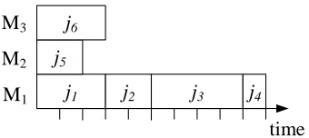
Consider an instance of the scheduling problem where J ={j1, j2, j3, j4, j5, j6},M =

{M1, M2, M3} and the processing times are p1 = 3, p2 = 2, p3 = 4, p4 = 1, p5 = 2, and

p6 = 3. The solution space includes all possible assignments of jobs to processors. As an

example, one possible solution S for this instance is shown in Figure 1.4, in which jobs

j1, j2, j3, j4 are processed by M1, j5 is processed by M2, and j6 is processed by M3. The

time needed by processor M1 to process jobs j1, j2, j3 and j4 (or the load of processor

M1) is 3 + 2 + 4 + 1 = 10. Similarly, the loads of processors M2 and M3 are 2 and 3,

respectively. The makespan of the schedule is equal to the maximum load, that in this instance is 10, which is also the time needed to process all the jobs.

j1 j2 j3 j4 j5

j6

time M1

M2

M3

Figure 1.4: Example of a scheduling problem.

In a local search algorithm we try to improve the current solution by performing a set of local operations. For this example we consider a local operation that moves a job from a processor with maximum load to a processor with minimum load; this operation is called the jump operation. Therefore, N(S) includes all the feasible solutions that are obtained from a solution S by performing a jump operation. In the above example one of the neighboring solutions of the solution S shown in the figure can be obtained by moving j1 to processor M2, which results in a reduced makespan. The processing time

of j1 is 3, therefore after performing this local operation the loads of the processors M1,

M2 and M3 change to 2 + 4 + 1 = 7, 2 + 3 = 5, and 3, respectively which decreases the

makespan to 7. We can further improve the makespan by moving j2 toM3 and this time

the load of all the processors is 5.

After the second jump operation we see that no further improvement is possible, since all the processors have equal load. Therefore, we obtained a local optimal solution, where no additional local operations can improve the cost. In this case the local optimal solution is also a global optimal solution because the total load created by all the jobs is 3 + 2 + 4 + 1 + 2 + 3 = 15 and we have 3 processors, therefore each processor must have load at least 5.

In the multiway cut problem [7] we are given a weighted graph G= (V, E) and a set

T ⊆V of terminals, whereV is a set of vertices andE is a set of edges with non-negative weights; the goal is to find a minimum weight setE0 ∈Ewhose removal fromGseparates all the terminals from one another, therefore partitioning V into |T| components each containing one terminal.

(19)

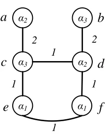
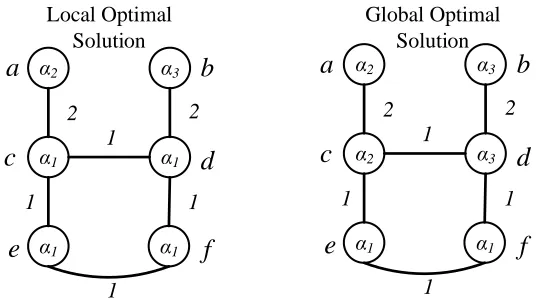
of a weighted graph with 6 vertices V = {a, b, c, d, e, f} and 3 terminals T = {a, b, e}. The goal is to partition the graph into 3 components each containing one terminal. The solution space includes all partitions of V that divide V into 3 parts and each part has exactly one terminal. In the figure we indicate vertices that belong to the same partition by assigning them the same label; for the example in Figure 1.5 the labels for the nodes in the three partitions are: α1, α2, α3and the label of each node is indicated inside the node.

Hence, the partitions shown in Figure 1.5 are{a, d},{b, c},{e, f}. The cost of the solution is 7 because the sum of the weights of the edges inE0 ={(a, c),(c, d),(b, d),(c, e),(d, f)}, whose removal creates this partition, is 7.

α2 α3

α3 α2

α1

a

c

e

2 2

1

α1

d

b

f

1

Figure 1.5: Initial solution for the minimum multiway cut.

Consider a local operation that changes the label of a single vertex. The neighborhood defined by this operation for a partitionP includes all the partitions that can be obtained fromP by changing the label of a single vertex. For the example shown in Figure 1.5 we can change the label of vertex c to α1, and as a result of this operation the cost of the

solution decreases by 1. If now we also change the label of vertex dtoα1 the cost further

(20)

α2 α3

α1 α1

α1

c

e

2 2

f

1

a

Local Optimal Solution

Global Optimal Solution

Figure 1.6: Local optimal solution and global optimal solution for the example of the multiway cut problem in Figure 1.5.

1.3 The Complexity of Computing Local Optimum

Solutions

Local search algorithms in some cases require a long time to compute local optimal so-lutions due to the fact that local operations could improve the cost of a solution by a very small amount. Let us, for example, consider the IterativeImprovement algorithm presented above. The time complexity of the algorithm depends on the number of itera-tions of the while loop and on the time it takes to find solution s0. Because there is no bound on the amount by which the value of a solution will improve in each iteration, we cannot guarantee a number of iterations that is bounded by a polynomial function of the size of the input.

Research has been conducted to determine the class of optimization problems for which local search algorithms have polynomial running times. Johnson, Papadimitriou, and Yannakakis [16] introduced a class of problems called PLS (polynomial-time local search problems) that admit local search algorithms with polynomial running times.

Orlin, Punnen and Shulz introduced the concept of-local optimum solution [19] that can be used to ensure polynomial running times for some local search algorithms, if a small loss in the quality of the solutions that it produces is tolerated. For a given constant value > 0, a solution s is -local optimum (for a minimization optimization problem) with respect to neighborhood function N if

c(s0)≥(1−)c(s) for each s0 ∈ N(s).

(21)

Choose a solution s0 ∈ N(s), where c(s0)<(1−)c(s).

Let sini be the initial solution selected by the IterativeImprovement algorithm and

sl be the -local optimal solution that it computes. For minimization problems, since

each iteration of the algorithm decreases the current solution s by at least × c(s), then the number of iterations of the while loop is Ologc(sini)−logc(sl)

. Since we are only interested in local search algorithms in which the neighborhood function can be computed in polynomial time, each iteration of the IterativeImprovement algorithm can be performed in polynomial time and so the algorithm runs in polynomial time. We can apply similar arguments to maximization problems as well.

Observe that the quality of an -local optimum solution is lower than that of a local optimum solution because for a minimization problem instead of each solution s0 ∈ N(s) satisfying the condition c(s0) ≥ c(s), where s is the local optimum solution, the

-local optimum solution s satisfies the weaker condition ₁₋1c(s0) ≥ c(s); therefore an

α-approximation local search algorithm yields an -local search algorithm that produces solutions of value within a factor ₁₋1α of the global optimal solutions. Similarly, for maximization problems an α-approximation algorithm can be converted into an -local search algorithm that gives solution of value within a factor (1 +)αof the global optimal solutions. In Chapter 2 we show how to use this notion of -local optimum to design a polynomial time local search algorithm for thek-facility location problem1_.

1.4 Local Search in the Design of Approximation

Al-gorithms

In spite of the conceptual simplicity of local search algorithms, they have not been used extensively for designing approximation algorithms. The two most significant reasons that make it difficult to design local search approximation algorithms for optimization problems are: First, computing the locality gap of a local search algorithm is complicated as we will see in Chapters 2, 3 and 4, and second, in some cases the locality gap of an algorithm is large and finding alternative local operations that would lead to efficient local search algorithms is difficult.

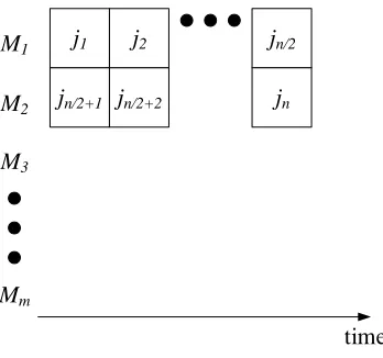
To clarify the second reason let us consider of the scheduling problem presented in Section 1.2. Consider an instance of this problem when the number of jobs n is an even multiple of the number mof processors, or in other words,n =km for some even integer

k > 0. Assume all jobs have unit processing time. If all the jobs are assigned evenly to only two processors,M1 andM2, as shown in Figure 1.7 then by using the jump operation,

as discussed in Section 1.2, the makespan cannot be improved; therefore, the solution given in Figure 1.7 is locally optimal with makespan km₂ . A global optimal solution for this example is obtained by distributing jobs evenly among all the processors and this achieves a makespan ofk. Therefore, the IterativeImprovement algorithm with the jump operation has a locality gap of at least km/_k2 = m₂, which is very large when m is big.

(22)

j1 j2 jn/2

jn/2+1 jn/2+2 jn

M1

M2

M3

Mm

time

Figure 1.7: Instance illustrating a big locality gap for a scheduling problem using the jump operation.

The problem with some local search algorithms is that they might get ”trapped” in a locally optimal solution that is far away from a global optimal solution. The above example clearly illustrates how this is possible. To address this problem, different classes of local search algorithms have been proposed such as: variable-depth search, tabu search, simulated annealing and genetic algorithms [4]. However, in this work we only consider iterative improvement algorithms. The other local search techniques are complicated and it is very difficult to compute their locality gaps. For the rest of this thesis ”local search” refers to iterative improvement.

Sometimes by using a different local operation we can improve the locality gap of a local search algorithm. For example, if we change the jump operation in the previous example in such a way that instead of moving only one job at a time we move up to

n jobs simultaneously then we can guarantee a locality gap of 1, or in other words this local search algorithm would be an optimal algorithm. We call a local search algorithms with locality gap 1 exact.

However, by changing the local operation the size of the neighborhood |N(s)| for a given solutionscan grow exponentially; hence, as a result of changing the local operation the time complexity of a local search algorithm can become exponential as it would be the case with the above jump operation that can move n job simultaneously. In the design of efficient local search algorithms besides achieving a small locality gap we need to achieve a reasonable time complexity.

(23)

1.5 Local Search Approximation Algorithms for

Com-binatorial Optimization Problems

In this section we give an overview of research that has been conducted on the design of local search approximation algorithms.

1.5.1 The Multiprocessor Scheduling Problem

As mentioned in Section 1.4 a problem with local search algorithms is that they might get trapped in a locally optimal solution that is far away from the global optimal one. Recall the example in Section 1.4 where two processors have the same maximum load and all other processor have load zero, and all other processor have lead zero and by performing a jump operation the makespan does not decrease.

To deal with this issue we can force the iterative improvement algorithm to continue performing jump operations on the jobs scheduled on processors with the maximum load. To achieve this, we define a new objective function c0 that assigns to every solution s a pair (c(s), `(s)), where c(s) is the makespan of s and `(s) is the number of processors with load c(s). Given two solutions s and s0, c0(s) < c0(s0) if c(s)< c(s0) or c(s) =c(s0) and `(s)< `(s0).

The neighborhood N(s) of s has size O(mn) because for all the n jobs there are

m−1 processors where a job can be moved (all processors except the processor on which the job is currently scheduled). Brucker et al. [3] show that the time complexity of the IterativeImprovement algorithm with the jump operation and cost functionc0 isO(mn3₎

and that its approximation ratio is 2− 1 m.

THEOREM 1 The IterativeImprovement algorithm with the jump neighborhood

func-tion and cost funcfunc-tion c0 has locality gap 2− 1 m.

Proof The proof that we give here for this theorem is very similar to the proof by

Graham for the approximation ratio of his List scheduling algorithm [12]. Let s be the local optimal solution computed by the IterativeImprovement algorithm and let s∗ be a global optimal solution. Let Mi be a processor with maximum load, let jr be the

last job processed by Mi and let t be the time when Mi starts to process jr; therefore,

c(s) = t+pr. Observe that since s is a locally optimal solution then no processor can

have load less than t. To see this let us consider that there is a processor Mk with load

lk < t; then by movingjr toMk we either obtain a solution with smaller makespan or we

reduce the number of processors with maximum load, contradicting the locality optimal condition. Therefore,

t≤ 1

m

X

ji∈J

pi−pr

!

≤c(s∗)− 1

(24)

as no solution can have makespan smaller than 1 m

P

ji∈Jpi. Therefore,

c(s) =t+pr ≤c(s∗)−

1

mpr+pr

=c(s∗) + (1− 1

m)pr

≤c(s∗) + (1− 1

m)c(s

∗

) as pr ≤c(s∗)

=c(s∗)(2− 1

m).

1.5.2 Computing a Spanning Tree with Many Leaves

Given a graph G = (V, E), a spanning tree of G is a subgraph of G that includes all vertices in V and it is a tree, i.e. it does not have any cycles. In a tree T we call all vertices with degree one leaves. We describe a local search approximation algorithm by Ravi and Lu [18] for the problem of finding a spanning tree with maximum number of leaves for a given graph G. The solution space of this problem includes all the spanning trees of the input graphG. The objective functionc(t) is the number of leaves in spanning tree t.

For a spanning tree t the exchange neighborhood of t includes all the spanning trees that differ from t by a single edge. Observe that the number of edges in a spanning tree

t is n−1, where n is the number of vertices of G. The exchange neighborhood of t is then defined as follows:

N(t) = {t0 |t0 is a spanning tree of G and |t∩t0|=n−2}.

For a given spanning tree t the local exchange operation replaces an edge of t with an edge inG−t that results in a new spanning treet0. Ravi and Lu showed that |N(t)| has size at most O(mn) and that the time complexity of their algorithm is O(mn2).

We do not show how to compute the locality gap for this algorithm as this analysis is much more complicated than for the above scheduling problem; the reason is that for the scheduling problem we could find a bound for the value of the global optimal solution that we could easily relate to the value of the local optimum solution. However, for the problem of finding a spanning tree with maximum number of leaves there does not seem to be a bound for the global optimal solution that can be easily related to the local optimal solution.

Ravi and Lu [18] showed that their algorithm has a locality gap of 10. In addition, they showed that by using a different local operation that allows the simultaneous exchange of two tree edges with two non-tree edges the locality gap can be improved to 3.

1.5.3 The

k

-Set Packing Problem

In the k-set packing problem we are given a finite set E of n elements and a collection

(25)

weighted version of this problem, called W-k-set packing, each set is assigned a cost and the goal is to find a maximum cost collection of pairwise disjoint sets. Both problems are NP-hard [11].

Perhaps the simplest approach to solve the W-k-set packing problem is a greedy ap-proach that starts with an initially empty collectionS, and then it adds to Sa maximum cost set B inF and removes fromF all the sets intersecting B. This process is repeated until the collection F becomes empty.

We show that the above greedy algorithm has approximation ratio k. Let S =

{S1, S2, ..., Sr}be the collection selected by the greedy algorithm and letS∗ ={S1∗, S

∗

2, ..., S

∗ p}

be an optimum solution. Sets in S are indexed in the order in which they were selected by the greedy algorithm. Then, for set S1 there are at most k sets in S∗ that have a

non-empty intersection with S1 because all the sets in S∗ are disjoint and have at most

k elements. Also, the cost of each one of these sets is no greater than that of S1. We

remove these sets from S∗. For set S2 there are at most k sets in the remaining sets of

S∗ that intersect it and their costs are no greater than the cost of S2 because otherwise

they would have been selected as setS2 by the greedy algorithm. Continuing in the same

manner we conclude that for each sett inS there are at mostk sets inS∗ that intersect it and have costs no greater than the costs of t. Therefore, the optimum solution has cost at most k times greater than the cost of S.

Chandra and Halld¨orsson [5] combined this greedy algorithm and a local search ap-proach to design an approximation algorithm for the W-k-set packing problem with locality gap (_nn₋₁)(4k₅+2). Their algorithm is a modification of the IterativeImprovement algorithm where they used the above greedy algorithm to find the initial solution.

1.5.4 The Max

k

-SAT Problem

LetB ={x1, x2, ..., xn} be a set ofn Boolean variables. A literal is defined to be either a

variable xi or its negation ¯xi,i= 1, .., n. In the MAXk-SAT problem we are given a set

of m boolean clauses C ={C1, C2, ..., Cm} where, each clause is a disjunction of exactly

k literals. The goal is to assign values to the variables so as to maximize the number of clauses that are satisfied. A clause is satisfied if its value is true.

Lets = (s1, ..., sn) be a vector that represent a solution to the MAXk-SAT problem,

i.e si is the value for variable xi. The flip neighborhood of s, N(s), consist of all the

solutions that can be obtained by changing only one value in vector s, i.e, by changing one value from true to false or vice versa.

Hansen and Jaumard [14] designed a local search algorithm for the MAX k-SAT problem with the flip neighborhood function and show that it has locality gap k+1_k .

1.5.5 The Traveling Salesman Problem

(26)

The optimum solution to the traveling salesman problem cannot be approximated within a constant factor in polynomial time unless P =N P [20]. However, if we assume that the weights of the edges satisfy thetriangle inequality, i.e. for any three edgese1,e2

ande3 forming a cycle of length 3 the sum of the weights of any two edges is greater than

or equal to the weight of the remaining edge, then it is possible to design approximation algorithms with constant approximation ratio. This problem is called the metric traveling salesman problem.

Given a cycle T, a cycle T0 is a 2-opt neighbor of T if it can be obtained from T by removing two edges from it and adding two new edges (see Figure 1.8).

Figure 1.8: An example of the 2-opt neighborhood.

Chandra, Karloff and Tovey [6] designed a local search algorithm with the 2-opt neighborhood for the metric traveling salesman problem and proved that it has locality gap 4√n, where n is the number of the vertices in G.

The related maximum weight Hamiltonian circuit is similar to the traveling sales-man problem, however instead of finding a minimum weight cycle the goal now is to find a maximum weight cycle. Fisher, Nemhauser and Wolsey [9] showed that a local search algorithm with the 2-opt neighborhood has locality gap 2 for the maximum weight Hamiltonian circuit problem.

1.5.6 The Quadratic Assignment Problem

In the quadratic assignment problem, denoted by QAP, we are given a set of facilities

Fs ={f1, f2, ..., fn}, a set of locations L={l1,12, ..., ln}, a flow matrix F = (fij), where

fij is the flow of material from facility i to facility j, and a distance matrix D = (dij),

where dkl is the distance from location k to location l. The cost of assigning facilities

i and j to locations k and l is defined to be fijdkl. The goal is to find an assignment

of facilities to locations, or in other words a permutation π that assigns a facility i to a location π(i), that minimizes the total cost of the assignment, given by the following sum

X

1≤i≤n

X

i+1≤k≤n

fikdπ(i)π(k). (1.4)

(27)

solution obtained by their local search algorithm and CAV is the average cost over all

possible solutions for any instance of QAP.

For a permutationπ= (π(1), π(2), ..., π(i), ..., π(j), ..., π(n)) the 2-exchange neighbor-hood ofπincludes all the n(n₂−1) permutations of the form (π(1), π(2), ..., π(j), ..., π(i), ..., π(n)) for 1≤i < j≤n obtained by performing a swap ofπ(i) andπ(j) in π.

1.5.7 The

k

-Set Cover Problem

In the k-set cover problem we are given a set U and a collection C of subsets of U each of size at mostk. The goal is to find a minimum size sub-collection of C whose union is

U. A set of size k is called a k-set. Without loss of generality we can assume that C is closed under subsets.

The (s, t)-neighborhood for a given solution S for this problem is determined by two values s, t >0 and includes all the solution S0 obtained fromS in two steps: First insert up tos3-sets intoSand delete up tot3-sets fromS. Since not all elements ofU might be covered after performing this first step, a second step is performed that optimally selects 2-sets and 1-sets to cover all the missing elements from U. The process of optimally selecting 2-sets and 1-sets for the second step can be done by modeling this problem as a maximum matching problem as follows. Construct a graphG= (V, E), whereV is the set of uncovered elements in U and E is determined by the 2-sets in C, i.e. if there is a 2-setA={a, b}inC then add an edge toE between the vertices corresponding toa and

b. The optimal 2-sets are selected by finding a maximum matching in G and the 1-sets are the remaining vertices that are not covered by the maximum matching (remember that C is closed under subsets).

The quality of a solution S is determined by the number of sets in S (a solution with fewer sets is better). An (s, t)-improvement is a move from a solutionS to a (s, t )-neighboring solution S0 with better quality. Duh and F¨urer [8] designed a local-search algorithm that uses (2,1)-improvements. They showed that their algorithm for the 3-set cover problem has a locality gap of 4

3 and that this bound is tight.

1.5.8 The Maximum Constraint Satisfaction Problem

To introduce the maximum constraint satisfaction problem, denoted MAX-CSP, first we define the notion of constraint satisfaction. For a given graphG= (V, E) anassignment

πis a function that assigns to each vertex a value from the setD ={1, ..., k}. Aconstraint

R(u, v) between vertices u and v defines a set of pairs of values that can be assigned to

uand v. A constraintR(u, v) issatisfied by assignmentπ if and only if (π(u), π(v)) is in

R(u, v).

In MAX-CSP we are given a graph G= (V, E) with a constraint R(u, v) associated with each edge (u, v) ∈ E, and a positive integer k; the goal is to find an assignment

π :V → {1,2, ..., k} such that the number of satisfied constraints is maximized.

A constraint R(u, v) is r-consistent for 1 ≤ r ≤ k if and only if, for every value

(28)

Halld´orsson [13] defined a neighborhood of an assignment π formed by all the as-signments obtained from π by changing the value of only one vertex. He showed that a local search iterative improvement algorithm with the above neighborhood function has approximation ratio r

k for MAX-CSP(k, r).

1.5.9 The Stable Marriage Problem

In the stable marriage problem (SM) we are given two sets, usually called men and women, each of size n. Elements of each set rank the elements of the other set. The goal is to find a matching between the two sets, i.e match each man with a woman, such that there are no two elements of opposite sex that prefer to be matched together than with their current matchings. A matching with this property is calledstable. There is a variant of the SM problem calledSMTI that allows ties and incompleteness. Ties allow indifference in the ranked list of each element and incompleteness allows each element to accept only certain subset of elements as partners.

A SMTI marriage M is a one-to-one matching between the two sets such that all

the matched elements accept each other. A woman w is matched with a man m inM if

M(m) =wand M(w) = m. If there is no match for a personpthen we callpsingle. The

marriage size, denoted|M|, is defined as the number of men (women) who have a match

in M. A blocking pair (m, w) in marriage M is a pair such that m and w accept each

other and m is either single in M or strictly prefers w than its current marriage M(m) and vice versa, i.e. wis either single in M or strictly prefersm than its current marriage

M(w). A marriageM is called a stable marriage if and only if it has no blocking pairs. The problem of finding the largest stable marriage is denoted as MAX SMTI and we now describe a local search algorithm for it. The neighborhood N(M) of marriage M

includes all the marriages that are obtained from M by finding a good partner for one of the single men in M. A good partner is a match such that the new couple does not create a blocking pair.

Iwama and et al. [15] designed a local search algorithm for the MAX SMTI problem with the above neighborhood and obtained a locality gap of 1.875. Their local search algorithm first selects an arbitrary matching M using the Gale-Shapley algorithm and then it repeatedly selects an appropriate neighbor from N(M) for the current matching

M.

(29)

1.5.10 Placement of Meters in Networks

To measure commodity flow on a flow network one could measure the flow on all the edges of the network; however, by using the flow conservation property we can achieve the same goal by only measuring the flow on the edges of any feedback edge set and then infering the flow on the remaining edges. A feedback edge set (FES) of a graph

G= (V, E) is a set E0 ⊆E whose removal converts a graph into an acyclic graph. The number of flow meters needed to obtain the flow on all the edges of a network is then equal to the number of edges in a FES. There is another option for measuring the flow on edges through the use of pressure meters. Pressure meters are placed on some nodes of the network and the flow on an edge is computed by measuring the flow pressure on the nodes incident to the edge. We could place the pressure meters on all the nodes of the network, however a more efficient solution is to put the pressure meters only on the nodes incident on an FES. Therefore, to minimize the number of meters needed, we wish to find a FES with the minimum number of nodes incident on it.

The problem of finding the minimum number of pressure meters on graphs is equiv-alent to the minimum vertex feedback edge set (VFES) problem, where given a graph

G= (V, E) the goal is to find a FES with minimum number of vertices incident on it. Khuller and et al. [17] showed that any minimal FES obtained by repeatedly deleting an edge from each cycle in the given graph has approximation ratio 3 and they also designed a local search algorithm with locality gap 2+_k1 using the following neighborhood function: for a given constantk the neighbors of a given FES f are all the feedback edge sets that differ from f by at mostk−1 edges.

1.6 Our Local Search Algorithms

We introduce in this section three combinatorial optimization problems that we have studied: k-facility location, multiway cut, and max k-cut. We also describe the local operations and neighborhood functions that we used in the local search algorithms that we designed for these problems.

1.6.1 The

k

-Facility Location Problem

In the k-facility location problem (k-UFL) we are given a set F of facilities, a set C of clients, service costsc, facility costs f, and an integer k bounding the maximum number of facilities that can be selected for servicing the clients. The goal is to select a set S of at mostk facilities to service the clients that minimizes the facility cost plus the service cost. Therefore, we want to minimize the following cost function,

cost(S) = Σi∈Sfi+ Σj∈Ccjσ(j), (1.5)

where S is set of at most k facilities, σ(j) is the facility in S with the smallest service cost to client j, fi is the cost of facility i and cjσ(j) is the cost of servicing client j. In

(30)

location problem. In the metric version of the problem the service costs satisfy the triangle inequality.

For example, consider the instance of the k-UFL problem shown in Figure 1.9. The facility costs are inside the nodes and the service costs are beside the edges. Let k = 3 andS ={s1, s2, s3}. The cost of solutionS is 22 because the facility cost is 4 + 4 + 4 = 12

and the service cost is 2 + 2 + 2 + 2 + 2 = 10.

We designed a local search algorithm for the k-UFL problem that uses a multi-swap

operation as local operation: Given a solution S for the problem, in a multi-swap op-eration we replace all the facilities in some set A ⊆ S with the facilities in another set

B ⊆F \S. Formally,

swap <A,B> := (S\A)∪B, whereA ⊆S and B ⊆F \S.

Consider the same instance of thek-UFL problem in Figure 1.9 and the above solution

S. Let A={s1, s2, s3} and B ={f1, f2, f3}. By performing swap <A,B> the cost of the

solution decreases from 22 to 8.

Using this local multi-swap operation the neighbors of a given solution S are all the solutions of the form (S\A)∪B, whereA⊆S and B ⊆F \S.

f1 f2 f3

s2

1 1 1 1 1

2 2 2 2 ₂

Facilities Clients

4

1 1 1

4 4

s1 s3

Figure 1.9: Example of a multi-swap operation, where S = {s1, s2, s3}, A ={s1, s2, s3}

and B ={f1, f2, f3}.

1.6.2 The Multiway Cut Problem

The multiway cut problem is another well-known combinatorial optimization problem, in which we are given a weighted graphG= (V, E), an integer k, and a set of terminals

T = {t1, t2, . . . , tk} ⊆ V. The goal is to divide the set V of vertices into k disjoint

partitions in such a way that each partition has exactly one terminal and the sum of the weights of the edges with endpoints in two different partitions is minimized.

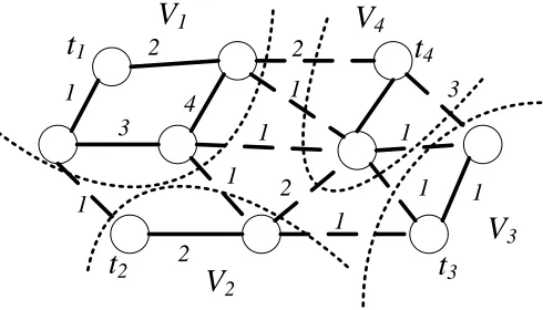
An instance of the multiway cut problem is shown in Figure 1.10, where k = 4 and

T ={t1, t2, t3, t4}. One possible solution for this instance of the problem is to divide the

vertices into the partitions V1, V2, V3, V4 shown in the figure. Let us call this solution

P. Let R be the set of edges crossing the partitions or, in other words, the edges that have their endpoints in two different partitions. These edges are drawn as dashed lines in Figure 1.10. The total weight of the edges inR is 14, therefore the cost of the solution

3

1

2

3 4

1

2 1

1 1

2

2 1

1 1

3

1

Figure 1.10: Instance of the multiway cut problem, where k = 4 andT ={t1, t2, t3, t4};

one possible solution for this instance of the problem is to divide the vertices into parti-tions V1, V2, V3, V4 and the cost of this solution is 14.

We designed a local search algorithm for the multiway cut problem that uses the

relabel operation as local operation. The relabel operation is easier to explain in the

context of labeling problems; therefore first we formulate the multiway cut problem as a labelling problem. In the labelling version of the multiway cut problem we are given a weighted graph G = (V, E), a set of terminals T = {t1, t2, . . . , tk} ⊆ V, and a set of

labels L = {l1, l2, . . . , lk}; the goal is to assign to each node a label from L in such a

way that the terminals have different labels and the sum of the weights of the edges that have their endpoints labelled with two different labels is minimized. An example of the labelling version of the multiway cut problem is shown in Figure 1.11, where k = 4 and

4

1

2

3 4

1

2 1

1 1 2

2 1

1 1

3

1

V

1

V

2

V

3

V

4

Figure 1.11: Instance of the labelling version of the multiway cut problem.

(32)

where all the nodes in partition Vi are assigned label li, and viceversa, a solution f to

the labeling problem determines a partitioning P in which all the nodes labeled li form

a partition Vi (see Figures 1.10 and 1.11).

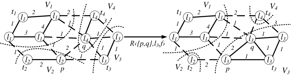
Given a labelling f for the vertices of a graphG= (V, E), a relabel operation changes the labels of the nodes in some setA ⊆V \T to a given label α leaving the labels of all other nodes unchanged. Formally, given a labellingf for the vertices, a set Aof vertices, and a label α, relabel operation RhA, α, fi is defined as follows,

2

_V

3

Figure 1.12: Example of a relabel operationRhA, α, fi, where A={p, q} and α =l3.

1.6.3 The Constrained Max

k

-cut Problem on Hypergraphs

Another well-known combinatorial optimization problem is the max k-cut problem. In the max k-cut problem we are given a weighted graph G= (V, E) and an integerk, and the goal is to divide the set V into k non-empty partitions in such a way that the sum of the weights of the edges having their endpoints in different partitions is maximized. An instance of the max k-cut problem is shown in Figure 1.13 where k = 4. Partition

P = {V1, V2, V3, V4} is one possible solution to the problem; the dashed edges are the

(33)

w V1

V2

V3 V4

Figure 1.13: Instance of the max k-cut problem.

A hypergraph H = (V, E) consist of a set V of nodes and a set E of hyperdges. A hyperedge e consists of a set of nodes or endpoints. The size of a hyperedge e is the number of its endpoints. Graphs are special cases of hypergraphs in which all the hyperedges have size 2.

In the max k-cut problem on hypergraphs the goal is to split the vertices into k

partitions in such a way that the sum of the weights of the hyperedges having at least two endpoints in different partitions is maximized. An instance of the maxk-cut problem on hypergraphs where k = 3 is shown in Figure 1.14. Let (u1, u2, . . . , ur) denote hyperedge

e where u1, u2, . . . , ur are its endpoints. The hypergraphH in Figure 1.14 consist of the

following hyperedges: e1 = (v1, v2), e2 = (v2, v3, v4), e3 = (v1, v5), e4 = (v4, v6, v7, v8)

and e5 = (v4, v5, v8). Let the weights of the hyperedges e1, e2, e3, e4, e5 are 2, 3, 1,

4, 1 respectively. The cost of the partition P = {V1, V2, V3} shown in Figure 1.14 is 9,

since each one of the hyperedges e2, e3, e4 and e5 have at least two endpoints located in

different partitions.

e1

e2 _e

4

e5

v1

v2