Practical Improvements of Profiled Side-Channel Attacks on a Hardware Crypto-Accelerator

(1)

Practical Improvements of Profiled Side-Channel

Attacks on a Hardware Crypto-Accelerator

–extended version

⋆

_–

M. Abdelaziz Elaabid1 _{and Sylvain Guilley}2

1

Université de Paris 8, Équipe MTII, LAGA 2 rue de la liberté, 93526 Saint-Denis Cedex, France.

2

Institut TELECOM / TELECOM ParisTech, CNRS LTCI (UMR 5141) D´epartement COMELEC, 46 rue Barrault, 75 634 PARIS Cedex 13, France. Email:

{elaabid,sylvain.guilley}@TELECOM-ParisTech.fr

Abstract. This article investigates the relevance of the theoretical frame-work on profiled side-channel attacks presented by F.-X. Standaert et al. at Eurocrypt 2009. The analyses consist in a case-study based on side-channel measurements acquired experimentally from a hardwired crypto-graphic accelerator. Therefore, with respect to previous formal analyses carried out on software measurements or on simulated data, the inves-tigations we describe are more complex, due to the underlying chip’s architecture and to the large amount of algorithmic noise. In this dif-ficult context, we show however that with an engineer’s mindset, two techniques can greatly improve both the off-line profiling and the on-line attack. First, we explore the appropriateness of different choices for the sensitive variables. We show that a skilled attacker aware of the regis-ter transfers occurring during the cryptographic operations can select the most adequate distinguisher, thus increasing its success rate. Sec-ond, we introduce a method based on the thresholding of leakage data to accelerate the profiling or the matching stages. Indeed, leveraging on an engineer’s common sense, it is possible to visually foresee the shape of some eigenvectors thereby anticipating their estimation towards their asymptotic value by authoritatively zeroing weak components containing mainly non-informational noise. This method empowers an attacker, in that it saves traces when converging towards correct values of the secret. Concretely, we demonstrate a 5 times speed-up in the on-line phase of the attack.

1 Introduction

Side-channel attacks are cryptanalytic techniques that exploit unintentional in-formation leakage from cryptographic devices during their operation. In the case of symmetrical encryption or decryption, side-channel attacks aim at recovering the secret key. As a consequence, there is a strong interest in efficient implemen-tation of countermeasures against such attacks. In the meantime, researchers

⋆

(2)

have tackled the difficult task to formalize the study of attacks and countermea-sures. A seminal theoretical study dealing with physical attacks is presented to the cryptographic community by S. Micali and L. Reyzin in [11]. In order to be practically usable, this paradigm requires a specialization, grounded on practical side-channel leakage simulations or measurements. This milestone is achieved by

F.-X. Standaertet al.in [21], where the information theory is solicited to process

the side-channel data. More precisely, in [21,20], F.-X. Standaertet al. discuss

two metrics to measure two independent aspects: the first is the robustness eval-uation of a target circuit and the second is the estimation of the power of an attack. For this purpose, two kinds of adversaries should be taken into consid-eration:

1. The adversary with an access to a certain amount of a priori information,

such as the circuit leakage model and the cryptographic algorithm being executed.

2. The adversary with an access to a clone of the attacked device. In this case, she would be free to manipulate it, in order to indirectly understand the behavior of the target device containing the secret information.

In this paper, we consider the second case. It unfolds in two stages. In a first stage of profiling, some estimations are carried out to extract information. In a second stage, a classification is carried out to perform the on-line attack.

The rest of the paper is organized as follows. Section 2 introduces the theo-retical notions employed in the forthcoming concrete analyses. The first attack improvement we investigate is related to the adequate choice of the sensitive variable. This study is detailed for both evaluation and attack metrics in Sec. 3. The second improvement concerns an analysis of the dates with maximal leakage. In Sec. 4, we indeed observe that a thresholding that anticipates the irrelevance of some side-channel samples is beneficial to both the evaluation and the attack metrics. A discussion about the impact of these two findings on the

interpreta-tion of the a priori evaluation metric and of the a posteriori attack metrics is

given in Sec. 5. Finally, conclusions and perspectives are in Sec. 6. The circuit whose side-channel signals are studied is presented in Appendix A.

2 Theoretical Framework for the Practice-Oriented

Side-Channel Study

2.1 Prerequisites

Based on some axioms, the theoretical analysis of the physical attacks detailed in [11] formalize the leakage by specifying “where, how, and when” the target circuit leaks information. Those axioms give a reliable description of the physical phenomena observable in practice. In this context, two technical definitions must

(3)

Leakage Function The leakage functionL(C, M, R) is a function of three

pa-rameters.Cis the current internal configuration of the circuit / algorithm, which

incorporates all the resources whose side-channels are measurable in principle;

M is a set of measures andR is a random string which represents the noise.

This function is an important element in the rest of this article. Indeed, from this notion we will create distinguishers that will enable us to evaluate the circuit by quantifying its side-channel information, or to be used by an adversary to recover the key.

Adversary In [11], the adversary is chosen so as to be the strongest possible and therefore can be different at each attack. In [20], the adversary uses a divide-and-conquer strategy to retrieve separately parts of the secret key. In other words,

it defines a functionf :K7→SK which maps each key konto a classsk=f(k)

such that |SK| ≪ |K|. The aim of a side-channel adversary is to guess a key

classsk with non negligible probability.

For example, in the case where the considered encryption algorithm is DES

(Data Encryption Standard), k will be the 56-bit key for encryption, and Sk

is the 6-bit subkey generated by the key schedule from the master key k and

consumed at the substitution box (sbox) input.

According to the given definitions, the evaluation of the physical security of a device is based on the quality of the circuit and the strength of the adversary. These two aspects urge to study the information quantity given by a leakage function. This will be taken advantage of to conduct a successful attack.

2.2 How to Quantify the Information Amount?

The concept of entropy was introduced by C. Shannon in [17]. It is a reliable measurement of uncertainty associated with a random variable. In our case, we use Shannon entropy to characterize the information leaked from a cryptographic device in order to extract its secret key. We denote by:

– SK the target key class discrete variable of a side-channel attack, and sK a

realisation of this variable;

– X the discrete variable containing the inputs of the target cryptographic

device, andx the realisation of this variable;

– L a random variable denoting the side-channel observation generated with

inputs of the target device, andl a realisation of this random variable;

– Pr[sK|L] the conditional probability of a key classsK given a leakagel.

One reason to quantify the information is to measure the quality of the circuit for a given leakage function. For this purpose, we use the conditional entropy, defined in Sec. 2.2. The other goal is to measure how brightly this information (leakage) is used to successfully recover the key. In the sequel, we consider the success rate, defined in Sec. 2.2, to assess the strength of the adversary.

(4)

The Conditional Entropy According to the definition of the conditional

Shan-non entropy, the conditional uncertainty ofSK givenL, denotedH(SK |L), is

defined by the following equations:

H(SK|L)=. X

sK

X

l

−Pr(sK, l)·log2Pr(sK |l)

=−X

sK

Pr(sK)

X

l

Pr(l|sK)·log2 Pr(sK |l). (1)

We the define conditional entropy matrix as:

HsK,sKc .

=−X

l

Pr(l|sK)·log2 Pr(sKc|l), (2)

wheresKandsKcare respectively the correct subkey and the subkey candidate.

From (1) and (2), we derive:

H(SK|L) = X

sK

Pr(sK)HsK,sK. (3)

The value of diagonal elements from this matrix needs to be observed very carefully. Indeed, theorem 1 in [21] states that if they are minimum amongst all

key classessK, then these key classes can be recovered by a Bayesian adversary.

The Success Rate The adversary mentioned in 2.1 is an algorithm that aims

at guessing a key classsK with high probability. Indeed with some queries, the

adversary would estimate the success rate from the number of times for which the attack is successful. The success rate quantifies the strength of an adversary and thereafter evaluates the robustness of a cryptographic device in front of its attack.

2.3 Profiled Side-Channel Attacks in Practice

There exist many operational contexts in which an attack can be setup. Some attacks consist solely of an on-line phase. The earliest attacks of this kind exploit explicitly the linear dependency between the secret data and the leakage, as in the Differential Power Attack (DPA, [9]) and the Correlation Power Analysis (CPA, [3]). Recently, the Mutual Information Analysis (MIA, [6]) has extended those attacks to non-linear dependencies. Profiled attacks are attacks mounted by a rather strong adversary that can benefit from a long period of training

(i.e.profiling) on a clone device, before launching the attack itself on the target

(5)

Template Attacks During the training phase the attacker gathers a large number of traces, corresponding to random values of plaintexts and keys. As the clone system is in full control of the attacker, this number is limited only by time and available storage. The observed traces are then classified according

to functions L that capture one modality of the circuit’s leakage. A trace t

is considered as the realisation of a multivariate Gaussian random variable in

RN_{. For each set}_S

k, k ∈[0, N′[ the attacker computes the averageµk and the

covariance matrixΣk. These are estimated by:

µk=

1

|Sk| X

t∈Sk

t and Σk=

1

|Sk| −1 X

t∈Sk

(t−µk)(t−µk)T. (4)

The ordered pair (µk, Σk) is called the template associated with value k of the

subkey.

The difficult part of this attack is the size of theΣkmatrices, namely (N×N),

withN ≈104_{. In our experiments,}_N _{= 20}_,_{000. To overcome this a few special}

indices can be chosen in [0, N[, called interest points, which contain most of the

useful information. Various techniques are used to select these points: points with large differences between the average traces [4], points with maximal variance [7],

and, more generally, principal component analysis (aka PCA [8].)

Template Attacks in PCA The PCA consists in computing the eigenvectors

EVi, i∈[0, N′[ of empirical covariance matrix of all traces together, computed

by:

S= 1

N′₋₁ N′−1

X

k=0

T TT _where _µ_¯₌ 1

N′ N′−1

X

k=0

µk and T = 

   

µT

1−µ¯T

µT

2−µ¯T

.. .

µT N −µ¯T



   

.

LetEV be the matrix containing the most significant eigenvectors. In practice,

only a few eigenvectors is sufficient to represent all data samples. In the case of our unprotected circuit, the leakage is well captured by one direction only,

irre-spective of the choice of the leakage functionL. The mean traces and covariance

matrices defined in (4) are then expressed in this basis by:

νk = (EV)Tµk and Λk= (EV)TΣk(EV).

In addition to the (EV) matrix, they constitute the templates of the PCA.

Theattack phase consists then in acquiring the traceτ of an encipherement

performed by the target system using the secret key κ, projecting it into this

latter basis and matching it against the patterns using Bayes’ rule. The attack is successful iff:

κ= argmaxk

1

p

(2π)N′_|_Λ

k|

exp

−1

2·(EV(τ−µk))

T_Λ−1

k (EV(τ−µk)) !

(6)

Applications of Templates in PCA to SecMat The investigations are done on an unprotected DES cryptoprocessor with an iterative architecture. We estimate the conditional entropy and the success rate for various leakage models: in fact, models are constructed from distinguishers for trace classification during the profiling attack. Altogether, this comparison will allow us characterize better the leakage.

We are facing the problem of choosing the relevant sensitive variable. Actually, it has already been pointed out, for instance in Section 2 of [20], that there are variables more sensitive than others from the attacker point of view. Thus, the security of a cryptographic device should not be treated generally, but must depend on each sensitive variable.

We must choose a variable that is sensitive (i.e. linked to the key) and

pre-dictable (i.e. the sizeN′

of the subkey is manageable by an exhaustive search). This leads to several questions:

– where to attack? For instance at the input or at the output of an sbox?

– plain values or distance between two consecutive values? In the latter case,

do we need the schematic of the algorithm implementation in the circuit?

– considering a transition as sensitive variable, is it worth considering the

Hamming distance instead of the plain distance3_?

To find the best compromise security / attacker, our experiments will attempt

to respond to these issues. We study the following leakage models.Model Ais

the input of the first sbox, a 6-bit model. Model B is the output of the first

sbox, a 4-bit model.Model C is the value of the first round corresponding to

the fanout of the first sbox, a 4-bit model.Model Dis the transition of model

C.Model Eis the Hamming weight of the model D.

We illustrate our study on the first round; the last round yields similar results. The mathematical definition of the models A to E is given in Tab. 1, using the notation of NIST FIPS 46 for the internal functions of DES and S as a shortcut

for S1||S2|| · · · ||S8. For a better readability, we also provide with a dataflow

illustration in Fig. 1.

We use the term “model” to designate the choice of the variable that depends on the plaintext or the ciphertext, and whose values determine the number of templates. This vocabulary can be misleading since it has also been used in the past to represent other quantities. In the original paper about the DPA [10], the model is actually called a “selection function”. In [14], the term “leakage model” qualifies the way a sensitive variable is concretely leaked; for instance, according to their terminology, the choice for the Hamming weight is a model of “reduction” of the sensitive variable. In this respect, they would say that E approximately models the leakage of D. We do not use this vocabulary, since we think that an attacker cannot tell the difference between an internal leakage and an externally observable one. This detail is rather a sophistication of the attack, best captured by the concepts behind the stochastic attacks [16]. The

3

Given two bitstrings x0 and x1 we call their plain distance the word x0⊕x1, as

(7)

Model Mathematical Abbre- Nature

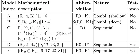
Dist-index description -viation -ance

A (R0⊕K1)[1 : 6] R0+K1 Combi. (shallow) No

B S(R0⊕K1)[1 : 4] S(R0+K1)Combi. (deep) No

C R1{9,17,23,31} =

P−1_(R₁_{)[1 : 4] = (S(R}₀ _⊕

K1))⊕P− 1

(L0))[1 : 4]

R1 Sequential No

D (R0⊕R1){9,17,23,31} R0+P1 Sequential Yes

E |(R0⊕R1){9,17,23,31}| |R0+R1| Sequential Yes

Table 1.The five leakage models confronted in this paper.

notion of “sensitive variable” is neither adequate, because it holds only if there is a straightforward link in the leakage and a value present in the algorithm specification (like our model A, B or C), Now, it seems difficult to qualify of sensitive variable a Hamming distance between two internal values taken by a sensitive variable, because it is unrelated to the algorithm itself. So, to sum up, we recall that we employ the term model to define the mapping between a trace and its template.

We note that these models can be viewed as two families of distinguishers. The models A and B are concerned with moments during the encryption, while models B, C and D focus on registers. Each studied case corresponds to one

number of templates. Model A uses 64 = 26 _{templates because it predicts the}

activity of the sbox input, whereas model B applies to 16 = 24_{templates that are}

the sbox output values. Models C and D are also made up of 16 templates, and finally, model E focuses on 5 templates that are classifications of the different values of a 4 bit Hamming distance.

The acquisition campaign consists in a collection of 80,000 traces. Half of

these traces are used for profiling and the other half for the on-line attack.

Tem-plates as shown above are in practice a set ofmeans and covariances for classes

constructed from models. In addition PCA allows to construct eigenvectors that

4 S

[1:4]

6

[1:6]

E 6

6

{32,1,2,3,4,5}

R0 P

4 R1

4

L1 ⊕_K1

6

{9,17,23,31} {9,17,23,31} [1:6]

[1:6]

Key(K1)

M

e

ss

a

g

e

(L

R0

)

⊕_L0

L0

{9,17,23,31} {32,1,2,3,4,5}

(8)

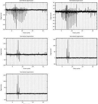
will be useful to reduce our data samples for online attack. In practice we use only the first eigenvector in order to project circuit consumption data. Indeed it is the most important vector since it relates to the greatest variance. We can also use the second or third eigenvectors if they are relevant, namely if they corre-spond to a large variance. Thus, we can increase the attacker’s strength. On the other hand, using a bad eigenvector only contributes to damage our attack. In figure 2 we can see the difference between a good (the second one) and a bad (the thirteenth one) eigenvector. With an unprotected circuit, it appears clearly that the leakage is well localized in time. Therefore a good eigenvector (corresponding to a high eigenvalue) is also almost null everywhere but at the leaking dates. We will take advantage of this property in the second improvement presented later on in Sec. 4.

According to the eigenvectors represented in Fig. 3, we can see precisely when our circuit leaks information in the modality A, B, D, E or F. The highest the eigenvector at a sample, the largest the leakage there.

3 Improvement of the Attacks thanks to an Adequate

Leakage Model

3.1 Success Rate

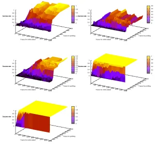
Success rates are depicted in Fig. 4 as a function of two parameters: the first one is the off-line profiling trace count and the second is the on-line attack trace count. For all curves, we notice that the success rate is an increasing function in terms of either trace count.

Model A seems better than B. Intuitively, we would have expected a similar attack performance, as the traversal of the sbox is a quasi-bijective function. This is not exactly true on DES, since the sbox of DES has a fanin of 6 and a smaller fanout of 4. However, they are designed in such a way that if two input bits are fixed, the sbox becomes bijective (in answer for a balancing requirement).

Therefore, the reason for B to be slightly worse than A is related to the implementation. Indeed, in the round combinational logic, B addresses a deeper leakage than A. Thus B is more subject to intra-clocking cycle timing shifts in the transitions and to the spurious glitching activity that characterizes the CMOS combinational parts.

Following this discussion, we could also expect the model C to be better than A, since C models the activity of a register. However, this is false in practice. One explanation is that the eigenvector of A has more peaks than that of C, and thus collects more information scattered in the trace.

(9)

-200 -150 -100 -50 0 50 100

8 16 24 32

Eigenvector

Clock cycles Normalized eigenvector

(a) Good eigenvector.

-40 -20 0 20 40 60

8 16 24 32

Eigenvector

(b) Bad eigenvector.

Fig. 2.Difference between “good” and “bad” eigenvectors for model B.

-80 -60 -40 -20 0 20

8 16 24 32

Eigenvector

-60 -50 -40 -30 -20 -10 0 10 20 30

8 16 24 32

Eigenvector

-100 -50 0 50 100 150

8 16 24 32

Eigenvector

-50 0 50 100 150

8 16 24 32

Eigenvector

-50 0 50 100 150

8 16 24 32

Eigenvector

(10)

0 0.2 0.4 0.6 0.8 1 0 500

1000 1500

2000 2500

3000

3500 4000 0

100 200 300 400 500 600 0 0.2 0.4 0.6 0.8 1 Success rate

Traces for online attack

Traces for profiling Success rate 0 0.1 0.2 0.3 0.4 0.5 0.6 0 500

1000 1500

2000 2500

3000

3500 4000 0 500

1000 1500

2000 2500

3000 3500

4000 0 0.2 0.4 0.6 0.8 1 Success rate

Traces for profiling Success rate 0 0.1 0.2 0.3 0.4 0.5 0.6 0.7 0.8 0.9 0

500 1000

1500 2000

2500

3000 3500

4000 0 500

1000

1500 2000

2500 3000

3500 4000

0 0.2 0.4 0.6 0.8 1 Success rate

Traces for profiling Success rate 0 0.2 0.4 0.6 0.8 1 0

500 1000

1500 2000

2500

3000 3500

4000 0 500

1000

1500 2000

2500 3000

3500 4000

0 0.2 0.4 0.6 0.8 1 Success rate

Traces for profiling Success rate 0 0.2 0.4 0.6 0.8 1

0 500

1000 1500

2000 2500

3000

3500 4000 0 500

1000 1500

2000 2500

3000 3500

4000 0 0.2 0.4 0.6 0.8 1 Success rate

Traces for profiling Success rate

(11)

were already evoked in the literature (for instance in [3] or in [20]), but never demonstrated. Through our experiment, we indeed formally concur on this point: distances between consecutive states are leaking more than values in CMOS cir-cuits.

0 0.2 0.4 0.6 0.8 1

0 200 400 600 800 1000 1200 1400 1600 1800 2000

success rate

online attack trace Model A [aka R0+K1] Model B [aka S( R0+K1)] Model C [aka R1] Model D [aka R0+R1] Model E [aka |R0+R1|];

(a)

0 0.2 0.4 0.6 0.8 1

0 50 100 150 200 250 300

success rate

online attack trace Model D [aka R0+R1] Model E [aka |R0+R1|];

(b)

Fig. 5. Success rate comparison, (a) between all models for the same number of pre-characterization traces and (b) between models D and E for the same number of profiling traces per class.

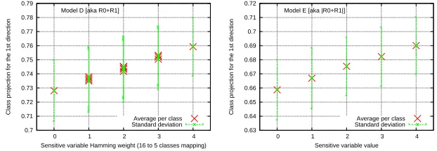
Eventually, we intend to compare models D (template-like [4]) and E (stochastic-like [16]). To be fair, we compute the success rate for a common number of traces

used in each template; namely, 16/5 more traces are required to profile D. The

result, given in Fig. 5(b) shows without doubt that D achieves better than E. The reason is that E is an approximate model. Figure 6 indeed shows that the de-generacy of identical Hamming weight classes is not perfect in practice; however, for a given number of measurements dedicated to profiling, E is favored.

0.7 0.71 0.72 0.73 0.74 0.75 0.76 0.77 0.78 0.79

0 1 2 3 4

Class projection for the 1st direction

Sensitive variable Hamming weight (16 to 5 classes mapping) Model D [aka R0+R1]

Average per class Standard deviation

0.63 0.64 0.65 0.66 0.67 0.68 0.69 0.7 0.71 0.72

0 1 2 3 4

Class projection for the 1st direction

Sensitive variable value Model E [aka |R0+R1|]

Average per class Standard deviation

(12)

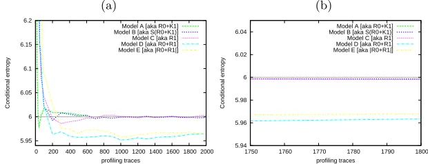
3.2 Conditional Entropy

As shown in Figure 7(a), the conditional entropy is roughly decreasing with the number of traces used in the profiling phase. We do not comment on the very be-ginning of the curves, since for small numbers of traces in the profiling phase, the entropy estimation yields false results. However, we notice that the conditional entropy tends towards a bounded value. As expected, this asymptotically value is less than or equal to 6 bits. Indeed, the keys we attack have 6 bits of entropy. The smaller the conditional entropy for a chosen model, the more vulnerable the circuit against one attack using this model.

(a) (b)

5.95 6 6.05 6.1 6.15 6.2

0 200 400 600 800 1000 1200 1400 1600 1800 2000

Conditional entropy

profiling traces Model A [aka R0+K1] Model B [aka S(R0+K1)] Model C [aka R1] Model D [aka R0+R1] Model E [aka |R0+R1|]

5.94 5.96 5.98 6 6.02 6.04

1750 1760 1770 1780 1790 1800

Conditional entropy

Fig. 7.Conditional entropy comparison. (a) over 2000 traces; (b) zoom after the estimation has converged.

In this comparison, we have tried to ensure having the same number of traces during the profiling phase. But this was not possible for model A that needs more measurements as it has more classes (64) than the others (16 or 5).

Therefore, we had the number of traces live in [0,600] for model A and in [0,2000] for the other models. By comparing the different models, it appears clearly that the models D and E are more favorable to side-channel leakage. Fig-ure 7(b) confirms that asymptotically, the conditional entropy for models D and E is smaller than other models, and that D is better than E. Therefore, the choice of the sensitive variable is an important element to be taken into account in a security evaluation. Basically, we observe that the conditional entropy classifies the models in the same order as the success rate.

(13)

But to sum up, this study of different models shows that the entropy is actually a good way to evaluate a circuit.

3.3 Hidden Models

We say that a leakage modelL1 is more adequate thanL2if the success rate of

an attack usingL1is greater than withL2. In the SecMat circuit we studied, the

distance between the consecutive values of a sensitive variables held in registers corresponds to the leakage function E. Discovering this better model is always possible, provided however that the attacker has a thorough knowledge of the cir-cuit’s architecture. More specifically, the value of a sensitive variable is accessible from anyone in possession of the algorithm specifications; on the contrary, the knowledge of the variables sequence requires that of the chip’s register transfer level (RTL) architecture, such as for instance its VHDL or Verilog description. Even in the absence of these pieces of information, an attacker can still attempt to retrieve the expression of the sensitive variables (or its sequence) as a function of the algorithm inputs or outputs, depending the attack is in known plaintext or known ciphertext context. Indeed, the attack acts as an oracle: if it fails to recover the key, it means that the leakage function is irrelevant. However, in hardware circuits, these functions are of high algebraic degree, especially when the next pipeline stage is a register that is one round inside the algorithm. This makes its prediction chancy, unless having some hints about a possible class of leakage functions. Refer to articles about SCARE [12,13] for a more complete overview of this problem.

We notice that the best leakage model (the most physical one) can be un-known willingly or as a backdoor. The algorithm pipeline can be indeed very complicated. Techniques to complexify the pipeline include:

– shuffling methods [?] can be used to randomize a pipeline. For instance,

the article [?] shows that the code of an algorithm can be rearranged in a

different order; even without taking advantage of any randomization, the high degree of commutativity ensures a high combinatorics in the algorithm scheduling, especially in software.

– masking of the sbox input / output with a constant, knowing that the sboxes

are the same for all the bytes of the datapath.

For the sake of completeness, we mention that the question of choosing the

adequate model has been raised for instance in this article [?]. There, the

au-thors contemplate to compare two generic countermeasure principles: hiding and masking. However, in their evaluation, they opted not to retain one common model for both countermeasure. Instead, a purported suitable model for each countermeasure is elected:

– a state-like model (similar to our model C) for the hiding countermeasure

and

– a distance-like model (similar to our model D) for the masking

(14)

As there is no state-of-the-art method to tell that the adopted model is indeed the best, the evaluation result remains biased. It holds provided an attacker indeed use these very models. However, if she does not restrict to this assumption, our

investigations show that the analysis done in [?] cannot be extrapolated to other

models.

4 Improvement of the Attacks thanks to Leakage Profiles

Noise Removal by Thresholding

As already emphasized in Fig. 2, an adversary able to understand the shape of the eigenvectors is more likely to master the speed of the success rate of her attack. In a similar way, a security evaluator may require an ideal eigenvector to have a very clear idea of the expertized device security.

In the case of a noisy vector, we must seek the best moments of leakage and eliminate the noise. In this context we suggest to improve the success rate

or degree of evaluation by creating a threshold th ∈[0,1] on the eigenvectors.

Generally speaking, in the case where we have infinite traces, the eigenvector will tend towards a denoised curve that reflects perfectly the temporal information for the leakage. In concrete evaluation and attack scenarios, we experience time or space constraints, and therefore we seek a better way to refine the eigenvectors.

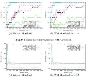
4.1 Success Rate

Figure 8(a) shows the significant gain which may be attributed to an adversary who perfectly knows how to exploit eigenvectors. This experiment was done with noisy traces different from those used in previous sections. The model chosen is the model A, which shows a significant increase in the rate of success (about

×5). There, the optimal threshold thopt is either 3/4 or 4/5 of the maximum

value of the eigenvector. Actually, we see that for an eigenvector whose noise is eliminated, the success rate becomes higher. Threshold choice is a compromise:

when it is too high (th ≈ 1), some noise remains, whereas when it is too low

(th≈0), it eliminates informative parts provided by the profiling phase.

Figure 8(b) shows on the example of model C how the success rate improves depending on the chosen threshold. For models of the same family (based on the value instead of on a distance), such as A and C, it can be noted that an adversary may be mistaken about the success rate, believing that such model is better than the other. In our case, if we do not take a threshold it is believed that the model A is better than C. However, with a thresholding, the conclusions are inverse, as depicted in Fig. 9.

4.2 Conditional Entropy

(15)

0 0.2 0.4 0.6 0.8 1

0 500 1000 1500 2000 2500 3000 3500 4000

Succes rate

online attack trace

without threshold threshold 3/4 threshold 4/5 (a) 0 0.2 0.4 0.6 0.8 1

0 200 400 600 800 1000 1200 1400 1600 1800 2000

success rate

online attack trace th=0 th=0.1 th=0.2 th=0.3 th=0.4 th=0.5 th=0.6 th=0.7 th=0.8 th=0.9 (b)

Fig. 8.Success rate comparison (a) without and with threshold for model A and (b) with different thresholds for model C.

0 0.2 0.4 0.6 0.8 1

0 200 400 600 800 1000 1200 1400 1600 1800 2000

success rate

(a) Without threshold.

0 0.2 0.4 0.6 0.8 1

0 200 400 600 800 1000 1200 1400 1600 1800 2000

success rate

(b) With thresholdth= 0.2.

Fig. 9.Success rate improvements with threshold.

5.95 6 6.05 6.1 6.15 6.2

0 200 400 600 800 1000 1200 1400 1600 1800 2000

Conditional entropy

(a) Without threshold.

5.95 6 6.05 6.1 6.15 6.2

0 200 400 600 800 1000 1200 1400 1600 1800 2000

Conditional entropy

(b) With thresholdth= 0.2.

(16)

5 Discussion

The goal of this section is to discuss the impact of the two improvement tech-niques to the side-channel framework of [21]. Basically, we warn that those two techniques can make an evaluation unfair if they convey an advantage dissym-metry to the attacker at the expense of the evaluator. To illustrate our argu-mentation, we resort to the same diagram as presented in [18]. The evaluator

(noted E) computes the x position whereas the attacker (noted A) computes

they position. This type of diagram can be seen as real worlda posteriori (i.e.

post mortem using forensic terminology) results as a function of forecasta priori

predictions.

For instance, it seems reasonable that some links between evaluation and attack metric can be put forward if they are computed on the same circuit with the same signal processing toolbox. Let us take the example of a chip we intend to stress, in order to exacerbate its leakage. Typically increasing the die’s

temperatureT (or its supply voltage) will increase its consumption and thus the

amount of side-channel. In these experiments, we expect the condition entropy and the attack success rate to evolve in parallel. And even more, this tendency should be independent on the chosen leakage model. These conclusions hold provided the temperature of the device during the evaluation is the same as during the attack. This is depicted in Fig. 11(a). Now, if the evaluator performs the evaluation at nominal temperature but that the attacker is able to attack at higher temperatures, he will be undoubtedly advantaged. This characterizes typically an asymmetric relationship between the attacker and the evaluator;

we can also say that the attacker “cheats”4 _{since she makes use of an extra}

degree of freedom unavailable to the attacker. This addition power changes the balance between the evaluation and the attack sides, as shown in Fig. 11(b). In concrete cases, for instance when the circuit to attack is a tamper-proof smartcard, the temperature, the voltage and all the operating conditions are

monitored. Therefore, a priori, neither the evaluator nor the attacker can be

advantaged.

The two contributions of this paper show however how to create a dissymme-try even when the evaluator and the attacker work in similar conditions (even better: on exactly the same traces [22]). The section 3 illustrates a situation

of dissymmetry in a priori knowledge. It is sketched in Fig. 12(a). When the

attacker knows that L2 is more adequate than L1, her attack will require in

average less traces to be successful than that of the evaluator that is stuck at

L1. The section 4 details the effect of a dissymmetry in expertise about the

ob-jects manipulated. Imagine a laboratory, such as an ITSEF, applying an attack “from the textbooks”, as presented in Sec. 2. Then this ITSEF faces the risk of overestimating the security of its target of evaluation if it is not aware of the thresholding “trick”.

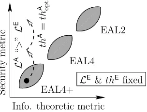
In summary, we warn that the evaluator can be fooled into being too confident in a circuit’s security, not having anticipated a weakness in the leakage model or

4

(17)

in the attack processing stages. Thus routine in the evaluation can be harmful in the projected trust in the circuit. This fact is illustrated in Fig. 13; if an evaluator has evaluated many cryptographic components that were found to lay within the

same region,e.g.corresponding to a common assurance evaluation level (“EAL”

notion of the Common Criteria [5]), he will be tempted to limit its analysis to the measurement of an information theoretic metric. However, if an attacker comes up with either more knowledge about the device that the evaluator does or better signal processing techniques, the previsions of the ITSEF can turn out be too optimistic, since conservative (believing erroneously that “anyone attacks like I do”).

Info. theoretic metric

S

ec

u

ri

ty

m

et

ri

c

TA_↑

TE_↑

TA_↓

TE_↓

TA₌_TE

S

ec

u

ri

ty

m

et

ri

c _TE_fixed

TA_↓

TA_↑

(a) (b)

Fig. 11. Evaluation vs attack metrics diagram in a (a) symmetrical and (b) asymmetrical situation.

Our two attack improvement techniques do not invalidate the framework of [21], but simply warn that the notions it introduces shall be manipulated with care and not overseen. Otherwise, incorrect predictions can be done, thus ruining the confidence we can have in it.

6 Conclusions and Perspectives

(18)

Info. theoretic metric S ecu ri ty m et ri

c thE_{= 1}

thA_{= 0}

thA_↓

thA₌thA

opt

thA_{= 1}

S ecu ri ty m et ri

c _LE_fixed

LA₌_LE

LA_“>_”_LE

(a) (b)

Fig. 12. Leakagevs attack diagram for our two attack optimizations: (a) ade-quate leakage models, (b) thresholding for non-informative samples.

00 00 00 00 11 11 11 11 000 000 000 000 111 111 111 111000 000 000 000 000 111 111 111 111 111 000 000 000 000 000 111 111 111 111 111000 000 000 000 111 111 111 111 000 000 000 000 000 111 111 111 111 111

S ec u ri ty m et ri c EAL4+ EAL4 EAL2

LE_&thE_fixed

L A “ > ” L E th A = th

A op

t

Fig. 13. Risk in trusting past experiences and relying on former evaluationvs

(19)

the perspective of the attacker, we provide two improvements over straightfor-ward attacks. First of all, we show that the care with which the sensitive variable is chosen influences qualitatively the attack outcome. In the studied hardware accelerator, the choice of the adequate sensitive variable is connected to its RTL architecture. Second, we illustrate that if the attacker knows that the leakage is localized in a few samples amongst the large number of sample making up the traces, she can intuit early (before the attack has converged to a unique key can-didate) that some samples will mostly bring noise instead of useful information. Thanks to an innovative thresholding technique, we show that by ruling those samples out, the attacker can indeed speed-up the attack. Finally, we conclude about the usefulness of the framework [21] in terms of security predictions when both the evaluator and the attacker can play with the same degrees of freedom. However, we warn that an attacker, especially in cryptography, can always come up with “out-of-the-box” strategies that might empower her with an advantage unanticipated by the evaluator.

Further directions of research will consist notably in assessing the question of the existence of an optimal leakage model. Or is the best evaluation / attack obtained from an analysis involving concomitantly many leakage models? But in this case, what technique is the most suitable to combine coherently various leak-age models? Techniques to exploit the side-channel information from multiple channels have already been presented. For instance, various EM are combined in [1]. Also, in [19], the simultaneous knowledge of power and EM leakage is taken advantage of to reduce the number of interactions with the cryptographic device under attack. However, in those two examples, the same leakage model is assumed. We endeavor in the future to get rid off this constraint. Additionally, we envision to port our techniques of leakage eigenvectors thresholding to attacks using an on-line profiling, such as the MIA [6], and to quantify the advantage it brings.

References

1. Dakshi Agrawal, Josyula R. Rao, and Pankaj Rohatgi. Multi-channel attacks. In CHES, volume 2779 ofLNCS, pages 2–16. Springer, 2003.

2. C´edric Archambeau, ´Eric Peeters, Fran¸cois-Xavier Standaert, and Jean-Jacques Quisquater. Template Attacks in Principal Subspaces. InCHES, volume 4249 of LNCS, pages 1–14. Springer, October 10-13 2006. Yokohama, Japan.

3. ´Eric Brier, Christophe Clavier, and Francis Olivier. Correlation Power Analysis with a Leakage Model. In CHES, volume 3156 ofLNCS, pages 16–29. Springer, August 11–13 2004. Cambridge, MA, USA.

4. Suresh Chari, Josyula R. Rao, and Pankaj Rohatgi. Template Attacks. InCHES, volume 2523 of LNCS, pages 13–28. Springer, August 2002. San Francisco Bay, USA.

5. Common Criteria consortium. Application of at-tack potential to smartcards v2-5, April 2008.

http://www.commoncriteriaportal.org/files/supdocs/CCDB-2008-04-001.pdf. 6. Benedikt Gierlichs, Lejla Batina, Pim Tuyls, and Bart Preneel. Mutual information

(20)

in Computer Science, pages 426–442. Springer, August 10-13 2008. Washington, D.C., USA.

7. Benedikt Gierlichs, Kerstin Lemke-Rust, and Christof Paar. Templates vs. Sto-chastic Methods. InCHES, volume 4249 ofLNCS, pages 15–29. Springer, October 10-13 2006. Yokohama, Japan.

8. Ian T. Jolliffe. Principal Component Analysis. Springer Series in Statistics, 2002. ISBN: 0387954422.

9. Paul C. Kocher, Joshua Jaffe, and Benjamin Jun. Differential Power Analysis. In Proceedings of CRYPTO’99, volume 1666 of LNCS, pages 388–397. Springer-Verlag, 1999.

10. Paul C. Kocher, Joshua Jaffe, and Benjamin Jun. Differential Power Analysis. In CRYPTO, volume 1666 ofLNCS, pages 388–397. Springer-Verlag, 1999. (PDF). 11. Silvio Micali and Leonid Reyzin. Physically observable cryptography. InTCC,

vol-ume 2951 ofLecture Notes in Computer Science, pages 278–296. Springer, February 19-21 2004. Cambridge, MA, USA.

12. Roman Novak. Side-channel attack on substitution blocks. InACNS, volume 2846 ofLNCS, pages 307–318. Springer, October 2003. Kunming, China.

13. Roman Novak. Sign-based differential power analysis. InWISA, volume 2908 of LNCS, pages 203–216. Springer, 2003. Jeju Island, Korea.

14. Emmanuel Prouff and Matthieu Rivain. Theoretical and Practical Aspects of Mutual Information Based Side Channel Analysis. In Springer, editor, ACNS, volume 5536 ofLNCS, pages 499–518, June 2-5 2009. Paris-Rocquencourt, France. 15. Werner Schindler. Advanced stochastic methods in side channel analysis on block ciphers in the presence of masking. Journal of Mathematical Cryptology, 2(3):291– 310, October 2008. ISSN (Online) 1862-2984, ISSN (Print) 1862-2976, DOI: 10.1515/JMC.2008.013.

16. Werner Schindler, Kerstin Lemke, and Christof Paar. A Stochastic Model for Differential Side Channel Cryptanalysis. In LNCS, editor,CHES, volume 3659 of LNCS, pages 30–46. Springer, Sept 2005. Edinburgh, Scotland, UK.

17. C. E. Shannon. A mathematical theory of communication. Bell system technical journal, 27, 1948.

18. F.-X. Standaert. A Didactic Classification of Some Illustrative Leakage Functions. InWISSEC, 1st Benelux Workshop on Information and System Security, page 16, November 8-9 2006. Antwerpen, Belgium.

19. Fran¸cois-Xavier Standaert and C´edric Archambeau. Using Subspace-Based Tem-plate Attacks to Compare and Combine Power and Electromagnetic Information Leakages. In CHES, volume 5154 of Lecture Notes in Computer Science, pages 411–425. Springer, August 10–13 2008. Washington, D.C., USA.

20. Fran¸cois-Xavier Standaert, Fran¸cois Koeune, and Werner Schindler. How to Com-pare Profiled Side-Channel Attacks? In Springer, editor, ACNS, volume 5536 of LNCS, pages 485–498, June 2-5 2009. Paris-Rocquencourt, France.

21. Fran¸cois-Xavier Standaert, Tal Malkin, and Moti Yung. A Unified Framework for the Analysis of Side-Channel Key Recovery Attacks. In EUROCRYPT, volume 5479 of Lecture Notes in Computer Science, pages 443–461. Springer, April 26-30 2009. Cologne, Germany.

22. TELECOM ParisTech SEN research group. DPA Contest (1st

edition), 2008–2009.

(21)

A

The SecMat V1 Evaluated Circuit

All the experimentations presented in this paper are carried out on measurements obtained from an ASIC implementation of DES, embedded in the “SecMat V1” chip, used notably for the DPA contest. The DES module is a straightforward

transposition in VHDL of the NIST standard [?]. It is iterative, in that it

com-putes one round of encryption per clock cycle.

The first round is indicated in the traces byt= 0, and therefore, the

cipher-text is ready at t = 15. In the Fig. 2, the variance is present mostly at clock