On Quantifying the Resistance of Concrete Hash Functions to Generic
Multi-Collision Attacks
Somindu C. Ramanna and Palash Sarkar
Applied Statistics Unit, Indian Statistical Institute,
203, B.T. Road, Kolkata, India 700108.
email: somindu [email protected], [email protected]
June 14, 2010
Abstract
Bellare and Kohno (2004) introduced the notion of balance to quantify the resistance of a hash functionhto a generic collision attack. Motivated by their work, we consider the problem of quantifying the resistance ofhto a generic multi-collision attack. To this end, we introduce the notion ofr-balance µr(h) ofhand obtain bounds on the success probability of finding anr-collision in terms ofµr(h). These
bounds show that for a hash function withmimage points, if the number of trialsqis Θ³rm(
r −1 r )µr(h)
´
, then it is possible to findr-collisions with a significant probability of success. The behaviour of random functions and the expected number of trials to obtain anr-collision is studied. These results extend and complete the earlier results obtained by Bellare and Kohno (2004) for collisions (i.e.,r= 2). Going beyond their work, we provide a new design criteria to provide quantifiable resistance to generic multi-collision attacks. Further, we make a detailed probabilistic investigation of the variation of r-balance over the set of all functions and obtain support for the view that most functions haver-balance close to one.
1
Introduction
An (n, m)-hash function is a map h:X →Y, where |X|= n, |Y| = m and n > m > 0. A collision for
h is a pair of distinct points x, x′ ∈ X such that h(x) = h(x′). Since n > m, collisions necessarily exist.
For cryptographic applications, h should be designed such that it is infeasible for a resource-bounded adversary to find a collision forh. Such a function is called collision resistant. The notion of a collision has been generalized to that of a multi-collision. Anr-way collision (or r-collision) consists of r distinct
domain points x1, x2,· · · , xr such that, h(x1) = h(x2) = · · · = h(xr). Again, for certain cryptographic
applications, the design goal is to ensure that for some suitable range ofr,r-collisions are hard to find for a resource-bounded adversary.
Given a hash functionh, an algorithm to find anr-collision forh is called an attack. A generic attack does not consider the manner in which the function h is defined, i.e., it does not consider the “internal structure” ofh. Instead, some points are picked from the domain and his applied to them with the hope that a subset of the points will yield anr-collision. In the context of generic attacks, the number of times
Suppose that q points x1, x2,· · ·, xq are picked. Then the probability of obtaining an r-collision
in-creases monotonically with q. The domain points on which to applyh can be chosen in different ways.
1. Sampling without replacement. An r-collision by definition requires the domain points to be distinct. Hence, one would like to use uniform random sampling without replacement to select the domain points. In particular,xi is selected uniformly at random fromX\{x1, . . . , xi−1}. Since it has
to be ensured thatxi is distinct from x1, . . . , xi−1, this method is not very convenient to implement.
Also, the lack of independence among thexi’s makes it more difficult to analyse this scenario.
2. Sampling with replacement. In this method the domain points are independent and uniformly distributed, i.e., xi is distributed uniformly over X and is independent of the previous choices.
From an algorithmic point of view, this is much more simpler to implement than sampling without replacement.
3. Picking distinct points without sampling. Suppose that h is a uniform random function from
X to Y. Then it is pointless to use a sampling strategy for picking the domain points. One can simply pick anyq distinct points, applyhto them and look for a collision. The probability of success does not depend on the particular set ofq points that has been picked. This can also be considered to be the uniform random distribution ofq balls to m bins and then looking for a bin with at least
r balls.
In this formulation, the problem has been studied in the literature. McKinney [McK66] gives an exact formula for the probability of findingr-collisions in q trials. But this formula gets more difficult to evaluate asrgrows. One can also express this probability using a multinomial cumulative distribution function. Levin [Lev81] provides an efficient way to compute a multinomial distribution function by expressing it as the conditional distribution of independent Poisson random variables given fixed sum. These approximations, however, provide little intuition on the asymptotic behaviour of the complexity of finding anr-collision. For r = 2, the complexity is Θ(m1/2) and the attack is usually called thebirthday attack.
Most works in the cryptography literature follow Point 3 above, i.e., these works ignore the actual hash function and instead analyse a random function. See for example the exposition in [Pre93] and the more recent consideration of the problem in [STKT06]. It is then (implicitly) implied that the results for a random function also hold for the actual hash function.
This approach has been eloquently criticised by Bellare and Kohno [BK04]. They argue that, given a concrete hash function h, one cannot assume that h has “random behaviour”, since then, one ends up “not analysing the given h, but rather analysing an abstract and ideal object which ultimately has no connection to h, regardless of the design principle underlyingh”.
The specific case of r = 2 (i.e., collisions) is considered in [BK04]. Suppose that the domain points
x1, . . . , xq are chosen using sampling with replacements as explained above. Then, it is usually assumed
that the birthday attack applies to the hash functionh. Bellare and Kohno [BK04] explain the drawback of this argument. Suppose that a point x is drawn uniformly at random fromX. Then it does not follow that the pointh(x) is uniformly distributed overY. Instead, the probability that ah(x) equals a particular
y∈Y is|h−1(y)|/|X|, whereh−1(y) is the set of all pre-images ofyunderh. So the pointsh(x
1), . . . , h(xq)
are uniformly distributed over Y if and only if h is regular, i.e., every range point has the same number of pre-images under h. This need not be true for the particular hash function under consideration. In fact, Bellare and Kohno [BK04] comprehensively cover textbook discussions of birthday attacks on hash functions and point out the inadequate and sometimes incorrect viewpoints that have been provided.
important measureµ(h), called thebalance of a hash functionh. This is defined to beµ(h) =−logm((n21+
· · ·+n2
m)/n2), whereY ={y1, . . . , ym}and ni is the number of pre-images ofyi. In other words,−µ(h) is
the logarithm of the probability thath(x) = h(x′) for x, x′ picked uniformly and independently fromX. Note that this includes the possibility thatx =x′ which is a trivial collision, i.e., −µ(h) is the logarithm of the probability of obtaining a possibly trivial collision. The rationale for considering possibly trivial collisions in the definition of balance is that ifnis large, then with high probability it is a proper collision. An extensive analysis is carried out to quantify the collision resistance of h in terms of the balance. To this end, two quantities are introduced: Ch(q) and Qh(c), where Ch(q) is the probability of finding a
collision inq trials andQh(c) = min{q :Ch(q) ≥c}is the minimum number of queries required to find a
collision with probabilityc. Bounds onCh(q) are obtained in terms of the balanceµ(h) and these bounds
are then translated to obtain bounds on Qh(c). Section 1.3 summarizes the bounds that they obtain.
They further show that regular functions offer (slightly) better collision resistance compared to random functions.
1.1 Our Contributions
The work done by Bellare and Kohno in [BK04] is forr= 2. We continue and to a certain extent complete the work started in [BK04] by considering r-collisions for arbitrary r ≥ 2. As noted above, like [BK04], we also work in the setting where the domain points are chosen according to uniform random sampling with replacement. We call this the generic multi-collision attack. The first question that we consider is the following.
What is the notion of balance of an (n, m)-hash functionh in the context ofr-collisions?
To answer this question, we introduceµr(h) which we call ther-balance of the functionh. This is defined
to be−(logmpr)/(r−1), wherepr is the probability thatr points chosen independently and uniformly at
random from the domain form an r-collision. For r1 < r2, we show the relation between r1-balance and
r2-balance. As in [BK04], the notion of r-balance then leads to the following question.
How is the performance of the generic multi-collision attack for finding r-collisions related to the notion ofr-balance?
Similar to [BK04], we study two quantities.
1. Ch(r)(q). This is the probability of finding an r-collision inq trials.
2. Q(hr)(c). This is the minimum number of queries required to find anr-collision with probabilityc.
Upper and lower bounds are obtained onCh(r)(q). These bounds onCh(r)(q) are translated to obtain upper and lower bounds onQ(hr)(c). From this it follows that for an (n, m)-hash function, the number of queries required to find anr-collision with significant probability is Θ(rmr−1
r µr(h)).
Following the agenda set out in [BK04], we next consider a uniform random (n, m)-hash function and introduce Cn,m$(r)(q) (resp. Q$(n,mr)(c)), which is the probability (resp. number of queries) for finding an r
-collision with q queries (resp. probability c). Again bounds on Cn,m$(r)(q) are obtained which are used to
obtain bounds onQ$(n,mr)(c). It is shown that if his a regular (n, m)-hash function, then for a certain range
of q, the upper bound on Ch(r)(q) is lesser than a lower bound on Cn,m$(r)(q). As a consequence, using the
Expected number of trials. In Section 4, we provide bounds on the expected number of trials to obtain an r-collision. For collisions, this was done by Bellare and Kohno and we adapt their general arguments to combine with the bounds obtained in this paper.
In an earlier work, Klamkin and Newman [KN67] consider the following problem: given m equally likely alternatives, repeatedly choose the alternatives one by one with replacements until one item occurs
r times. They study the expected number of trials for this event to occur and show that as m goes to infinity the expected number of trials is approximately rΓ(1 + 1/r)m(r−1)/r, where Γ denotes the usual
Gamma function defined by
Γ(u) =
Z ∞
0
e−xxu−1dx.
In Section 4.2, we show the relation between this problem and finding r-collisions for a concrete hash function. In the process, we generalise their approach to work when the alternatives are not necessarily equally likely.
Textbook discussion. Most textbooks analyse collisions obtained by the birthday attack. As mentioned earlier, inadequacies of such analysis has been discussed in [BK04]. On the other hand, to the best of our knowledge, no textbook analyses r-collisions with respect to the generic multi-collision attack. The only analysis available in the literature is using the “balls and bins” approach as discussed above.
Relation to the work of Bellare and Kohno [BK04]. At a general level, we follow the path set out in [BK04]. Some of the results that we obtain for generalr have, in a way, been already anticipated by the results for r= 2 in [BK04]. Having said this, we would also like to note that our analysis and proofs are not straightforward extensions of [BK04]. Some of the important differences are noted below.
Definition of balance. A straightforward extension of the Bellare and Kohno’s definition of balance will be based on the logarithm of (nr1+· · ·+nrm)/nr. The quantity (nr1+· · ·+nrm)/nr is the probability thath(x1) =· · ·=h(xr) whenx1, . . . , xrare sampled with replacement from the domain. This would
include possibly trivialr-collisions, i.e., it would include the possibility that xi =xj for somei6=j.
The definition ofr-balance that we define is based on the probability of actual r-collisions and not possibly trivial r-collisions. As we show later, this probability is ((n1)r +· · ·+ (nm)r)/nr, where
(ni)r =ni(ni−1)· · ·(ni−r+ 1). This expression is somewhat more complicated, but, we are able to
satisfactorily analyse it. The advantage is that our bounds are better than what would be obtained otherwise.
Lower bound on the success probability. In [BK04], the lower bound onCh(q) is shown to hold only
for a certain range ofq.
In contrast, the lower bound on Ch(r)(q) that we obtain holds for all q. This is a consequence of the fact that Ch(r)(q) is monotone increasing in q. (Similarly, Ch(q) is also monotone increasing in q,
but, [BK04] do not consider the consequences of this fact.)
Upper bound on the number of queries. The lower bound on success probability translates into an upper bound on the number of queries.
We note an issue of interpretation. In [BK04], it is mentioned that the bounds onQh(c) are meaningful
probabilityc. But, we still can say that at least a certain number of queries will be required to obtain success probabilityc.
Going beyond the Bellare-Kohno agenda. There are two main issues that are considered in this work but have not been considered in [BK04].
1. One criticism about the notion ofr-balance is that it is impractical to compute its value for practical hash functions. This may be considered to limit the usefulness of the notion. Our argument against this is twofold.
First, the notion of r-balance helps in exactly pinning down the resistance of a hash function to generic multi-collision attack. This highlights its central role in our understanding of multi-collisions which is important irrespective of whether one can compute the value or not.
Second, and from a more practical point of view, we show that this notion leads to a possibly new design criteria for practical hash functions. Suppose that a designer wishes to provably ensure a certain degree of resistance to r-collision attacks, i.e., the designer wishes to prove that finding r -collisions must require a minimum number of hash function evaluations. In Section 2.6, we show that using the notion ofr-balance one can satisfactorily give a rather precise answer to this question. In particular, we show that if the number of pre-images of any range point is bounded above, then
r-balance has a provable lower bound which translates into a provable lower bound on the number of hash function evaluations to find anr-collision using the generic attack.
2. An important question regarding r-balance is whether most functions have r-balance close to one. We make a detailed investigation of this question using a probabilistic approach. The balance of a random function is a random variable. Probability concentration bounds for this random variable is obtained using Markov inequality, Chebyshev inequality and Chernoff bound. This allows us to support the view that most functions haver-balance close to one.
1.2 Related Work
The property ofr-collision freeness has been suggested as a useful tool in building cryptographic protocols. It has been used for the micropayment scheme Micromint of Rivest and Shamir [RS96], for identification schemes by Girault and Stern [GS94] and for signature schemes by Brickellet. al. [BPVY00].
The intuition behind relying onr-collision freeness is that finding multi-collisions is harder than finding collisions. This is true when the function is truly random. But concrete hash functions mostly lack “random behaviour”. For the case of hash functions based on an iterated construction, Joux [Jou04] has demonstrated that r-collisions in iterated hash functions are not much harder to find than ordinary collisions, even for very large values ofr. Following Joux’s attack, several works [NS07, HS06] have extended the attack to more general classes of constructions.
There are several space efficient algorithms that find cycles in random graphs. These methods can be used to find collisions in a hash function. It would be interesting to find space efficient algorithms to find multi-collisions. This problem has been addressed recently by Joux and Lucks in [JL09]. They give an algorithm to find 3-collisions that roughly usesmδ storage and whose running time ism1−δ forδ ≤3. This shows that finding 3-collisions in timem2/3 would requirem1/3 units of storage.
1.3 Bounds Obtained by Bellare and Kohno [BK04]
Theorem 1.1. [BK04] Leth be an(n, m)-hash function andm≥2. Letα ≥0be any real number. Then for any integerq ≥2
(1−α2/4−α)·
µ q
2
·
µ
1
mµ(h) −
1
n 
≤Ch(q)≤ µ
q
2
·
µ
1
mµ(h) −
1
n 
, (1)
the lower bound being true under the additional assumption that
q ≤α·³1−m
n ´
·mµ(h)/2. (2)
Theorem 1.2. [BK04] Let h be an (n, m)-hash function andn≥2m≥4. Letα≥0 be any real number such thatβ = 1−α2/4−α >0. Let c be a real number in the interval 0≤c <1. Then
√
2c·mµ(h)/2 ≤Qh(c)≤1 + r
4c
β ·m
µ(h)/2, (3)
the upper bound being true under the additional assumption that
c≤(α·(1−m/n)−m−µ(h)/2)2·β
4 . (4)
2
Balance-Based Analysis of the Generic Multi-Collision Attack
The generic multi-collision attack that we consider is the following. Given an (n, m)-hash function h :
X→Y do the following.
1. Pickx1, . . . , xq independently and uniform at random fromX.
2. Compute yi=h(xi) for 1≤i≤q.
Anr-collision is found if there are indicesi1, . . . , irwith 1≤i1 < i2 <· · ·< ir≤qsuch thatyi1 =· · ·=yir
andthe domain points xi1, . . . , xir are distinct. To find anr-collision we certainly needq ≥r.
Our goal here is to analyse the performance of the generic multi-collision attack in terms of what we call ther-balance ofh. Equivalently, we want to analyse how the following quantities vary withr-balance.
• Ch(r)(q): probability that anr-collision forhis found inqtrials (q≥r). This function is monotonically increasing in q since the probability of finding r-collisions cannot decrease as the number of trials increases.
• Q(hr)(c): the minimum number of trials required to obtain anr-collision with probability greater than or equal toc. That is,
Qh(r)(c) = min{q:Ch(r)(q)≥c}. (5) Higher the value of c, more is the number of trials needed to find an r-collision. Hence Q(hr)(c) is monotonically increasing inc.
2.1 Notation
If d is a non-negative integer, then [d] = {1,2,· · ·, d}. For an integer r ≥ 2, [d]r denotes the set of all r-element subsets of [d]. [d]r,2 denotes the set of all 2-element subsets of [d]r. Let r ≥ 2 and d ≥ 0 be
integers. Then (d)r is defined as follows.
(d)r = ½
d(d−1)· · ·(d−r+ 1) if d≥r
0 otherwise
Let h : X → Y be an (n, m)-hash function. For any y ∈ Y, h−1(y) = {x ∈ X : h(x) = y}. Let
Y ={y1, y2,· · ·, ym}. Then fori∈[m], ni =|h−1(yi)|denotes the size of the set of pre-images ofyi under h.
2.2 Definition of r-Balance
A natural way to define ther-balance of h would be in terms of the probability of finding r-collisions for
h. To this end, we first prove the following result.
Proposition 2.1. Let h : X → Y be a hash function whose domain X and range Y = {y1, y2,· · ·, ym} have sizesn, m≥r, respectively. Fori∈[m], letni=|h−1(yi)|denote the size of the pre-image ofyi under h. Let r elements be chosen independently and uniformly at random from the domain X. The probability that they form anr-collision is
pr=
Pm
i=1(ni)r
nr .
Proof. Letr elements w1, w2,· · · , wr be picked independently and uniformly at random from the domain X. LetEbe the event that these elements form anr-collision. LetAdenote the event that these are distinct and for 1≤i≤m, letBi be the event thath(w1) =· · ·=h(wr) =yi. ThenE =AB1∪AB2∪ · · · ∪ABm.
Since Bi’s are mutually exclusive events, we have
Pr[E] =
m X
i=1
Pr[ABi] = m X
i=1
Pr[A|Bi]·Pr[Bi] = m X
i=1
ni(ni−1)· · ·(ni−r+ 1) nr
i ·
nri nr
=
m X
i=1
ni(ni−1)· · ·(ni−r+ 1) nr
Sincepr= Pr[E], the proposition follows.
Definition 2.1. Let h :X → Y be a hash function with |X|= n and Y = {y1, y2,· · ·, ym}. Let n≥ r
and pr>0. The r-balance of h, denoted µr(h), is defined as
µr(h) = 1
r−1 ·logm
µ
1
pr 
. (6)
If ni < r for alli, then there cannot be any r-collisions, that is,pr= 0. A necessary condition for the
existence of anr-collision is thatni≥r for at least onei. Ifn≥rm, then an r-collision will certainly exist
Consider the caser = 2. From the definition ofµ(h), we have
m−µ2(h) =
Pm
i=1ni(ni−1)
n2 =
Pm
i=1ni2
n2 −
Pm
i=1ni
n =m
−µ(h)
−n1.
This shows that µ2(h) is always greater than µ(h). The difference gets smaller as ngrows larger.
The following lemma will be useful in obtaining bounds on ther-balance of a hash function.
Lemma 2.2. Let r ≥2 be an integer. Let n1, n2,· · · , nm be non-negative integers such that Pmi=1ni =n. Then
m·³n m
´
r ≤ m X
i=1
(ni)r ≤(n)r.
The upper bound is attained when exactly one of the ni equals n and all others are zero, while the lower bound is attained when all the nis are equal.
Proof. We will prove the bounds using a counting argument. Let S(ni) denote the set of all distinct
arrangements ofni things takenr at a time. Then|S(ni)|= (ni)r fori= 1,· · ·m. Ifnj ≤r−1 for somej
thenS(nj) =∅. Assume, without loss of generality, that the firstkof the ni’s are greater than r−1. By
definition n =Pmi=1ni. Let S denote the set of all distinct arrangements of n things taken r at a time.
Each arrangement in S(ni) is also present in S. This shows that S(n1)∪S(n2)∪ · · · ∪S(nk) ⊆S. Also
since theS(ni)’s are disjoint, we have
(n1)r+ (n2)r+· · ·+ (nk)r≤(n1+n2+· · ·+nk)r= (n)r
Equality occurs whenk = 0 i.e., one of theni’s is equal to nand the rest are zero. This gives the upper bound onPmi=1(ni)r.
Now we claim thatPmi=1(ni)rattains its minimum when allni’s are equal i.e.,n1 =n2 =· · ·=nm= mn.
Suppose there exist ni and nj such that ni > mn and nj < mn. Assume, without loss of generality, that i= 1 and j= 2. To prove the claim, we need but show that
(n1−1)r+ (n2+ 1)r+· · ·+ (nk)r<(n1)r+ (n2)r+· · ·+ (nk)r.
LetTi denote the set containingni items. Clearly,T1∪T2∪ · · · ∪Tm=X. Letx∈T1. The number of
arrangements of items inT1 takenr at a time that containx is equal tor(n1−1)r−1. Suppose we remove
xfromT1 and put it inT2. Then the number of arrangements of items inT2 takenr at a time that contain
xis equal to r(n2)r−1. Thus we have
((n1)r+ (n2)r+· · ·+ (nk)r)−((n1−1)r+ (n2+ 1)r+· · ·+ (nk)r)
= |S(n1)∪S(n2)∪ · · · ∪S(nm)| − |S(n1−1)∪S(n2+ 1)∪ · · · ∪S(nm)|
= |S(n1)∪S(n2)| − |S(n1−1)∪S(n2+ 1)|
= |S(n1−1)|+r(n1−1)r−1+|S(n2)| − |S(n1−1)| − |S(n2)| −r(n2)r−1
= r(n1−1)r−1−r(n2)r−1
> 0
sincen1−1> n2. This gives the lower bound.
The following proposition provides the minimum and maximum values of the r-balance of a function and the conditions under which they are attained. The proof follows directly from the definition ofµr(h)
Proposition 2.3. Let h be an(n, m)-hash function. Then
1
r−1logm
nr
(n)r ≤
µr(h)≤
1
r−1logm
nr
m·¡mn¢r (7)
The lower bound is attained when h is a constant function and the upper bound is attained when h is a regular function.
Letµminr (n, m) andµmaxr (n, m) denote the minimum and maximum values of ther-balance of an (n, m )-hash function. The quantity µminr (n, m) can be approximated as follows.
µminr (n, m) = 1
r−1logm
nr
(n)r
= 1
r−1logm
1
¡
1−n1¢· · ·¡1−r−n1¢
≈ 1
r−1logm
1
e−1/n· · ·e−(r−1)/n =
1
r−1logm 1
e−(r2)/n
= r 2n(lnm).
This shows that, for large n, theµminr (n, m) is close to zero. Similarly one can approximateµmaxr (n, m) as follows.
µmaxr (n, m) = 1
r−1logm
nr
m·¡mn¢r =
1
r−1logm
mr−1 ¡
1− m n ¢
· · ·³1−(r−n1)m´
≈ r 1
−1logm
mr−1
e−m/n· · ·e−(r−1)m/n
= 1
r−1logm
³
mr−1e(r2)m/n
´
= 1 + rm 2n(lnm).
This shows that for large n,µmaxr (n, m) is close to one.
2.3 Relation Between r1-Balance and r2-Balance
One natural question that arises is whether it is easy to find r2-collisions for a given hash function given
thatr1-collisions can be found easily, forr16=r2. We will analyse this by looking at the difference between
the r1-balance and r2-balance of the function. In the following discussion, we will write µr in place of µr(h).
Proposition 2.4. Let h be an(n, m)-hash function withn1 ≥n2 ≥ · · · ≥nm where the ni’s are as defined earlier. Let 2≤r1 < r2 ≤n1. Let nj be the smallest among the ni’s which is greater than or equal to r2.
Let the function fr1,r2 be defined as follows:
fr1,r2(x) = (x−r1)(x−r1−1)· · ·(x−r2+ 1).
Then µ
r2−1
r1−1
¶ µr2 −
1
r1−1
logm n
r2−r1
fr1,r2(nj)
≤µr1 ≤
µ r2−1
r1−1
¶ µr2 −
1
r1−1
logm n
r2−r1
fr1,r2(n1) .
Proof. Let r1 be fixed. We will prove this result using induction on r2. For the base case, suppose that
r2 =r1+ 1 =r, say.
(nj −r+ 1)
m X
i=1
(ni)r−1 ≤
m X
i=1
(ni)r ≤(n1−r+ 1)
m X
i=1
(ni)r−1. (8)
From the definition ofr-balance we have
(r−1)µr−(r−2)µr−1= logmn+ logm
Pm
i=1(ni)r−1
Pm
i=1(ni)r
. (9)
Combining inequality (8) and Equation (9) we get
logm n
n1−r+ 1 ≤
(r−1)µr−(r−2)µr−1 ≤logm n nj−r+ 1 µ
r−1
r−2
¶ µr−
1
r−2logm
n nj −r+ 1≤
µr−1≤
µ r−1
r−2
¶ µr−
1
r−2logm
n n1−r+ 1
. (10)
This completes the proof of the base case. Suppose now that the result holds forr2−1. We need to show
that it holds forr2. First, consider the lower bound. By induction hypothesis we have
µr1 ≥
µ r2−2
r1−1
µr2−1−
1
r1−1
logm n
r2−r1−1 fr1,r2−1(nj)
. (11)
Inequality (10) gives us a lower bound onµr2 as follows:
µr2−1 ≥
µ r2−1
r2−2
¶ µr2−
1
r2−2
logm n
nj−r2+ 1
.
Substituting this lower bound in inequality (11), we get,
µr1 ≥
µ r2−2
r1−1
¶ µµ r2−1
r2−2
¶ µr2 −
1
r2−2
logm n
nj −r2+ 1
− 1
r1−1
logm n
r2−r1−1 fr1,r2−1(nj)
=
µ r2−1
r1−1
¶ µr2−
1
r1−1
logm n
r2−r1
(nj−r2+ 1)fr1,r2−1(nj)
=
µ r2−1
r1−1
¶ µr2−
1
r1−1
logm n
r2−r1
fr1,r2(nj) .
Applying the same technique to the upper bound, we get the required result.
The following corollary follows directly from Proposition 2.4 and is simpler to understand.
Corollary 2.5.
¯ ¯ ¯ ¯µr1−
µ r2−1
r1−1
¶ µr2
¯ ¯ ¯ ¯<
1
r1−1
logm n
r2−r1
fr1,r2(nj)
≤ r 1
1−1
logm n
r2−r1
fr1,r2(nm) .
We can interpret Proposition 2.4 as follows: Ifr2collisions can be found easily for a given hash function,
then it is not much harder to find r1 collisions for r2 > r1. If r1-balance (resp. r2-balance) is known for
a function, then one can get some idea of the valuer2-balance (resp. r1-balance). Note that the bounds
coincide for regular and constant functions.
Note. If r2-collisions do not exist, then we cannot say anything about how hard it is to findr1-collisions.
For example, consider a function for which (r+1)-collisions do not exist. Thenni≤rfor alli∈ {1,· · ·, m}. Finding r-collisions for functions of such form is not necessarily easy. If ni =r for alli(and so n=rm),
2.4 Bounds on Ch(r)(q)
ForI ∈[q]r,I ={i1, i2,· · ·, ir}, define a random variable ZI as follows.
ZI = ½
1 ifxi1, xi2,· · · , xir form anr-collision
0 otherwise
From Proposition 2.1 and the definition of r-balance we have
E[ZI] = Pr[ZI = 1] =
Pm
i=1(ni)r
nr =m
−(r−1)µr(h)=pr (12)
Then Z =PI∈[q]
rZI denotes the number ofr-collisions. The expected value of Z is
¡q r ¢
m−(r−1)µr(h).
We are interested in an r-collision and would like to know the number of queries required to have the expected value of Z to be equal to 1. This is given by the value of q such that (q)r = r!×m(r−1)µr(h).
Using the inequality (q−r)r <(q)
r, it can be easily shown that choosing q =r+ (r!)1/r×m(r−1)µr(h)/r
ensures that E[Z]≥1. This gives an indication of the “right” value ofq required to obtain anr-collision.
We now consider that q trials are made and obtain bounds on Ch(r)(q). An upper bound on Ch(r)(q) is easy to obtain.
Theorem 2.6 (Upper Bound onCh(r)(q)). Let h be an(n, m)-hash function withn≥r and m≥2. Then for any integerq ≥r,
Ch(r)(q)≤
µ q r
pr. (13)
Proof. Let {i1, . . . , ir} ⊆[q]. The probability that xi1, . . . , xir forms an r-collision is pr. The result now
follows from the union bound on probability.
To obtain a lower bound onCh(r)(q), we need the following lemma.
Lemma 2.7. Let h be an(n, m)-hash function and ℓ be an integer such that ℓ > r. Then
à m
X
i=1
(ni)ℓ !r
≤
à m
X
i=1
(ni)r !ℓ
. (14)
As a consequence,pℓ≤pℓ/rr .
Proof. Without loss of generality assume that n1 ≥ n2 ≥ · · · ≥ nm. Let Ai = (ni)ℓ, Bi = (ni)r and Ci = (ni−r)· · ·(ni−ℓ+ 1), so thatAi=BiCi. We are required to show
(B1C1+· · ·+BmCm)r ≤(B1+· · ·+Bm)ℓ. (15)
Consider the multinomial expansion of the left hand side of this equation. A term of this expansion is of the form
r!
d1!d2!· · ·dm!
(B1C1)d1(B2C2)d2· · ·(BmCm)dm
whered1+· · ·+dm =r. We show that this term is less than or equal to ℓ!
(d1+ℓ−r)!d2!· · ·dm!
Bd1+(ℓ−r)
1 B2d2· · ·Bmdm
1. d r!
1!d2!···dm! ≤
ℓ!
(d1+ℓ−r)! d2!···dm!.
2. (B1C1)d1(B2C2)d2· · ·(BmCm)dm≤B1d1+(ℓ−r)B2d2· · ·Bmdm.
Point (1) holds if r!
d1! ≤
ℓ!
(d1+ℓ−r)!,i.e., if
ℓ(ℓ−1)· · ·(r+ 1)
(d1+ℓ−r)(d1+ℓ−r−1)· · ·(d1+ 1) ≥
1.
This inequality holds if for 1≤j≤ℓ−r,r+j≥d1+j which clearly holds sinced1≤r.
Now consider the second point, which holds if Cd1
1 C2d2· · ·Cmdm ≤ B1ℓ−r. For 1 ≤ j ≤ ℓ−r, let Ej =
(n1−r−j+ 1)d1· · ·(nm−r−j+ 1)dm. Clearly Ej ≤E1 for 1≤j≤ℓ−r. Then, it follows that
Cd1
1 C2d2· · ·Cmdm=E1E2· · ·Eℓ−r≤E1ℓ−r
Point (2) now follows ifE1≤B1. Using the assumption thatn1 ≥ni for 1≤i≤m, it follows that
E1 = (n1−r)d1· · ·(nm−r)dm ≤(n1−r)d1+···+dm = (n1−r)r≤(n1)r=B1
This completes the proof of (14). By definition,
pℓ=
Pm
i=1(ni)ℓ
nℓ ≤
(Pmi=1(ni)r)ℓ/r
nℓ =
µ Pm
i=1(ni)r nr
¶ℓ/r
=pℓ/rr .
This completes the proof.
Theorem 2.8 (Lower Bound onCh(r)(q)). Let h be an(n, m)-hash function with n≥r and m≥2. Then
Ch(r)(q)≥ 1
2
Ã
2−
r−1
X
k=0
µ r k
¶µ q−r r−k
pr(r−k)/r !
·
µ q r
·pr. (16)
Proof. Let [q]r,2 denote the set of all 2-element subsets of [q]r. By the principle of inclusion and exclusion,
we have
Ch(r)(q) = Pr
_
I∈[q]r
ZI= 1
(17)
= X
I∈[q]r
Pr[ZI = 1]− X
I,J∈[q]r
I6=J
Pr[ZI = 1∧ZJ = 1]
+ · · · + (−1)(qr)−1Pr
^
I∈[q]r
ZI = 1
(18)
Considering the first two terms in the above equation will give us a lower bound onCh(r)(q).
Ch(r)(q)≥ X
I∈[q]r
Pr[ZI= 1]− X
{I,J}∈[q]r,2
X
I∈[q]r
Pr[ZI = 1] = µ
q r
Pr[ZI = 1] = µ
q r
·pr (20)
In order to obtain the required lower bound, we need to maximize the second term of Equation (19). This is where our proof deviates from the one given in [BK04].
For k = 0,1,· · · , r−1, let Tk be the number of pairs {I, J} ∈ [q]r,2 such that |I ∩J| = k. The k
common elements can be chosen in¡qk¢ ways. The remaining r−k elements in I can be chosen in ¡qr−−kk¢ ways and for each suchI, we can choose the remainingr−kelements inJ in¡qr−−rk¢ways. But this way we are counting every unordered pair twice (i.e.,{I, J}and{J, I}are indistinguishable but both are counted). Therefore, we have
Tk =
1 2
µ q k
¶µ q−k r−k
¶µ q−r r−k
= 1 2
µ q r
¶µ r k
¶µ q−r r−k
(21)
We can now break up the second term in Equation (19) as follows:
X
{I,J}∈[q]r,2
Pr[ZI = 1∧ZJ = 1] = r−1
X
k=0
Tk·Pr[ZI = 1∧ZJ = 1|(|I∩J|=k)] (22)
Let xI and xJ denote the set of points corresponding to the index sets I and J respectively. Suppose I
and J are disjoint (i.e., k= 0). Due to the disjointedness of I and J and the sampling strategy, the value
ZI takes is independent of the valueZJ takes. So when k= 0, we have,
Pr[ZI = 1∧ZJ = 1] = Pr[ZI = 1]·Pr[ZJ = 1] =pr2. (23)
When k≥1, the eventsZI = 1 andZJ = 1 indicate that the elements in xI map to a common point and
so do the elements inxJ. Since I∩J =6 ∅, the common image of the elements of both xI and xJ must be
the same. Hence Pr[ZI = 1∧ZJ = 1|(|I ∩J|= k)] is the probability that the 2r−k distinct elements corresponding to the index setI∪J form a 2r−k-collision. That is,
Pr[ZI = 1∧ZJ = 1] =p2r−k (24)
Combining Equations (21), (22), (23) and (24), we obtain the following:
Pr[ZI = 1∧ZJ = 1] =T0·pr2+
r−1
X
k=1
Tk·p2r−k (25)
To obtain an upper bound on the above expression, we need an upper bound onp2r−k. From Lemma 2.7,
we have
p2r−k≤pr(2r−k)/r =prpr(r−k)/r. (26)
Combining Equations (21), (25) and (26), we obtain
X
{I,J}∈[q]r,2
Pr[ZI = 1∧ZJ = 1]≤
1 2
µ q r
·pr· r−1
X
k=0
µ r k
¶µ q−r r−k
pr(r−k)/r (27)
2500 5000 7500 10000 12500 15000 17500 0.01
0.02 0.03 0.04 0.05
50000 100000 150000 200000 250000 300000 0.0005
0.001 0.0015 0.002 0.0025 0.003
Figure 1: Behaviour ofL(hr)(q) for r= 2 and r= 3 with m= 232 and µ
r= 0.9.
Ch(r)(q) ≥
µ q r
·pr−
1 2
µ q r
·pr· r−1
X
k=0
µ r k
¶µ q−r r−k
pr(r−k)/r
= 1 2
µ q r 
·pr· Ã
2−
r−1
X
k=0
µ r k
¶µ q−r r−k
pr(r−k)/r !
Towards a better lower bound. We now discuss the behaviour of this lower bound. Let
s(hr)(q) = 2−
r−1
X
k=0
µ r k
¶µ q−r r−k
pr(r−k)/r
and let the lower bound of Theorem 2.8 be denotedL(hr)(q). We have
L(hr)(q) = 1 2·pr
µ q r
¶ s(hr)(q).
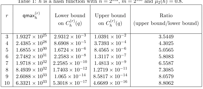
Table 1: his a hash function with n= 2512,m= 2160 and µ
2(h) = 0.8.
r qmax(hr) Lower bound Upper bound Ratio
on Ch(r)(q) on Ch(r)(q) (upper bound/lower bound)
3 1.9327×1025 2.9312×10⁻³ 1.0391×10⁻² 3.5449
4 2.4385×1028 8.6908×10⁻⁵ 3.7393×10⁻⁴ 4.3025 5 1.6855×1030 1.6724×10⁻⁶ 8.4565×10⁻⁶ 5.0565 6 2.7482×1031 2.2583×10⁻⁸ 1.3117×10⁻⁷ 5.8083
7 1.9718×1032 2.2585×10⁻¹⁰ 1.4813×10⁻⁹ 6.5587 8 8.4939×1032 1.7403×10⁻¹² 1.2719×10⁻¹¹ 7.3085 9 2.6088×1033 1.065×10⁻¹⁴ 8.5817×10⁻¹⁴ 8.0579
10 6.3321×1033 5.3018×10⁻¹⁷ 4.6689×10⁻¹⁶ 8.8062
• The binomial coefficient¡qr¢= r1!q(q−1)· · ·(q−(r−1)) and it vanishes at the points 0,1,· · · , r−1 which means these are roots ofL(hr)(q). It is also monotone increasing and positive for q≥r.
• s(hr)(q) is decreasing in q and becomes negative after a certain point causing L(hr)(q) to decrease.
• The polynomial s(hr)(q) has exactly one sign change and by Descartes’ rule of signs it will have at most one positive real root.
These observations show thatL(hr)(q) has exactlyr+ 1 non-negative real roots including 0,1,· · ·, r−1. This is because L(hr)(q) is positive at q = r and after a certain point becomes negative which means it is zero at exactly one point afterr−1. Let the (r+ 1)st real root be denoted as θ. In the interval ranging from q = r to q = θ, the curve representing L(hr)(q) must have one turning point. Figure 1 gives some examples to show howL(hr)(q) behaves. Let the value ofqat which the curve turns be denotedqmax(hr)and let cmax(hr) =Lh(r)(qmax(hr)). For q ≤qmaxh(r) the lower bound will be L(hr)(q). For q >qmax(hr),L(hr)(q) is decreasing but the probability of finding r-collisions cannot decrease as we increase the number of trials. Hence L(hr)(qmax(hr)) is a better lower bound. Based on this discussion and Theorems 2.6 and 2.8, we are able to state more appropriate bounds onCh(r)(q).
Theorem 2.9. Let h be an(n, m)-hash function. Then
max
r≤t≤qL
(r)
h (t)≤C
(r)
h (q)≤ µ
q r
·pr. (28)
Note. Theorem 2.9 is valid for allq (and for allr ≥2). This is to be contrasted with the bound obtained in [BK04] for the caser= 2 (see Theorem 1.1).
the bounds increases. The table indicates that the bounds are quite close. The ratio increases by around 0.75 with every one-step increases inr.
The lower bound stated in Theorem 2.9 can be further simplified as shown below.
Corollary 2.10. Let h be an (n, m)-hash function. Assume n≥r ≥2. Let
α(q) =qm−(r−1
r )µr(h). (29)
ThenCh(r)(q)≥ max
r≤t≤q
1
2 (3−(α(t) + 1)
r)·µt r
·m−(r−1)µr(h).
Proof. We proceed as in the proof of Theorem 2.8 upto Equation (27). It is after this point that the proof will deviate. Using Equations (19), (20) and (27) we get
Ch(r)(q) ≥
µ q r
·pr−
1 2 µ q r 
·pr· r−1
X k=0 µ r k ¶µ q−r r−k
pr(r−k)/r
= 1 2 µ q r 
·pr·
Ã
2−
r−1
X k=0 µ r k ¶µ q−r r−k
pr(r−k)/r !
≥ 12
µ q r 
·pr· Ã
2−
r−1
X k=0 µ r k 
qr−kpr(r−k)/r ! = 1 2 µ q r 
·pr·
Ã
2−
r−1
X k=0 µ r k 
(α(q))r−k
! = 1 2 µ q r 
·pr·(2−((α(q) + 1)r−1))
= 1 2 µ q r 
·pr·(3−(α(q) + 1)r).
Using the same arguments that led to Theorem 2.9, we get the bound stated in Corollary (2.10).
This simplification actually weakens the bound sinceqr−k is a weak upper bound on¡q−r r−k ¢
but can make it easier to work with the expressions.
2.5 Bounds on Q(hr)(c)
Now we obtain upper and lower bounds onQ(hr)(c). These bounds can be directly obtained from the bounds onCh(r)(q).
Theorem 2.11. Let h be an(n, m)-hash function withn≥r and m≥2. Let τ =s(hr)(qmax(hr)). Let c be a real number such that0≤c <1. Then
c1/r³r e
´ m(r−1
r )µr(h)≤Q(r)
h (c)≤ µ
2c τ
¶1/r
·rm(r−1
r )µr(h), (30)
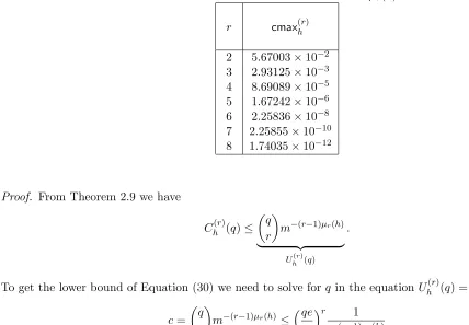
Table 2: h is a hash function withm= 280 andµ
r(h) = 0.9.
r cmax(hr)
2 5.67003×10⁻² 3 2.93125×10⁻³ 4 8.69089×10⁻⁵
5 1.67242×10⁻⁶ 6 2.25836×10⁻⁸ 7 2.25855×10⁻¹⁰
8 1.74035×10⁻¹²
Proof. From Theorem 2.9 we have
Ch(r)(q)≤
µ q r
m−(r−1)µr(h)
| {z }
Uh(r)(q)
.
To get the lower bound of Equation (30) we need to solve forq in the equationUh(r)(q) =c.
c=
µ q r
m−(r−1)µr(h)≤³qe
r
´r 1
m(r−1)µr(h)
and so q≥c1/r¡r e ¢
m(r−1
r )µr(h).This proves the lower bound of Equation (30).
Similarly the upper bound can be obtained by finding the minimum value of q such that L(hr)(q) ≥c. Since the maximum value ofL(hr)(q) iscmaxh(r) the minimum suchqwill be less thanqmax(hr). By definition,
sh(r)(q) is decreasing in q which implies sh(r)(q) > τ for q <qmax(hr). Combining this with Theorem 2.9 we have forq ≥qmax(hr),
Ch(r)(q)≥ max
r≤t≤qL
(r)
h (t)≥
1 2s
(r)
h (q)· µ
q r
·pr ≥ 1
2s
(r)
h (q)· ³q
r ´r
pr ≥ τ
2 ·
³q
r ´r
pr.
If q is such that Ch(r)(q) ≥(τ /2)(q/r)rpr ≥ c, thenQh(r)(c) ≤ q. Let the minimum suchq be denoted q∗. Clearlyq∗ is a solution to (τ /2)(q/r)rp
r=c. The upper bound on Q(hr)(c) follows from this.
Theorem 2.11 establishes our claim that the number of trials required to find r-collisions with a sig-nificant probability of success is Θ³rm(r−1
r )µr(h)
´
. For a given hash function h, the number of trials required to obtain an r-collision with a given probability c is at least as much as the lower bound. Also for c ≤ cmax(hr), the number of trials required to obtain success probability c will not exceed the upper bound onQ(hr)(c). For values ofcgreater thancmax(hr) we are unable to say anything about the maximum number of trials required to attain success probabilityc. But, the lower bound still continues to hold, i.e., we are still able to say that at least those many queries will be required to attain success probabilityc.
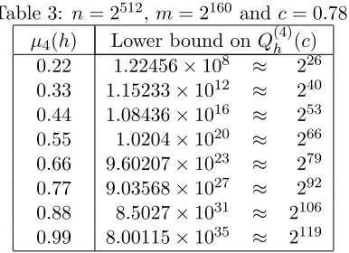
Table 3: n= 2512,m= 2160 andc= 0.78.
µ4(h) Lower bound on Q(4)h (c)
0.22 1.22456×10⁸ ≈ 226 0.33 1.15233×10¹² ≈ 240
0.44 1.08436×10¹⁶ ≈ 253 0.55 1.0204×10²⁰ ≈ 266 0.66 9.60207×10²³ ≈ 279
0.77 9.03568×1027 ≈ 292 0.88 8.5027×1031 ≈ 2106 0.99 8.00115×1035 ≈ 2119
cmax(hr). Table 2 shows how cmaxh(r) varies with r when m and µr(h) are fixed. One can observe that the
value of cmax(hr) is decreasing rapidly with increasing values of r which means that asr grows larger the upper bound of Theorem 2.11 is valid across smaller ranges ofc.
Sensitivity of Q(hr)(c) to r-balance. We provide some computational results that indicate how the number of trials required by the generic multi-collision attack changes according to the r-balance of the function being attacked. Table 3 shows the lower bound on Q(4)h (c) for a fixed c and for functions with different values of 4-balance. The table indicates that for functions with higher 4-balance it is harder to find 4-collisions using the generic multi-collision attack when compared to functions with low 4-balance.
2.6 Applicability of our Results
It is practically infeasible to compute or estimate the r-balance of a given hash function. In [BK04], the authors address this question for the case r = 2. Some experiments are performed on SHA-1 and the balance is computed considering only small blocks of the output string. The details are as follows. Let
SHAn :{0,1}n → {0,1}160 denote the restriction of SHA-1 to inputs of length n <264. Let SHAn;t1···t2 :
{0,1}n→ {0,1}t2t1+1denote the function that returns thet
1-th throught2-th output bits ofSHAn. Bellare
and Kohno ask what exactly is the balance ofSHA32;t1···t2 when t2−t1+ 1∈ {8,16,24} and whether the
functions SHAm;t1···t2, m ∈ {160,256,1024,2048}, appear regular when t2 −t1 + 1 ∈ {8,16,24}. They
calculate the balance ofSHA32;t1···t2 for all pairs t1, t2 such that t2−t1+ 1∈ {8,16,24} and t1 begins on
a byte boundary (i.e., they look at all 1-, 2-, and 3-byte portions of theSHA-1 output). The values they calculate indicate that, for the specified values oft1,t2 , the balance of SHA32;t1···t2 is high.
However, these experiments do not provide any information about the balance of the actual SHA-1. Instead of pondering over how to compute the r-balance of a given function, we discuss what could be done to ensure a hash function has certainr-balance.
Proposition 2.12. A hash function will have r-balance at least ν, if it is constructed in such a way that no range point has more than n/m(ν(r−1)+1)/r pre-images.
Proof. Essentially, we want the following to hold:
µr = 1
r−1logm
nr
Pm
or equivalently, Pmi=1(ni)r ≤ nrm−(r−1)ν. Suppose that for all i ∈ {1,2,· · · , m}, ni ≤ n/mδ for some δ∈[0,1]. Then
m X
i=1
(ni)r ≤m
³ n
mδ ´
r ≤m
³ n
mδ ´r
.
To ensure r-balance at least ν, it is enough if δ is such that m³ n mδ
´r
≤ nrm−(r−1)ν. Solving for δ, we obtain,δ ≥(1/r)×(ν(r−1) + 1).This completes the proof.
So while building a hash function with r-balance at least ν, the designer must ensure that no range point has more than n/m(ν(r−1)+1)/r pre-images. According to Theorem 2.11, this makes sure that an
attacker will need at least c1/r(r/e)mν(r−1)/r trials to obtain an r-collision with probability at least c. From Proposition 2.4, ensuring a lower bound on r2-balance also provides a lower bound on r1-balance.
So, a designer can pick a suitable r2 and ensure that the hash function has a high enough r2-balance.
For example, suppose we want a 256-bit hash function with 180-bit security against the generic multi-collision attack for 4-collisions. In other words, we would like the attack to make at least 2180 queries to ensure that a 4-collision is obtained with a constant probability of success c. So, we require
c1/r(r/e)mν(r−1)/r >2180 wherem= 2256 and r = 4. Taking logarithms to base two and assumingc≈1,
under reasonable approximations, the 4-balance µ4 must be at least (4/3)×180/256 = 0.9375. We can
ensure this by designing the function in such a way that every range point has at leastn×2−244pre-images. Clearly, this method can be extended for higher values ofr.
3
Random Functions
In this section, we consider a uniform random (n, m) function. Our purpose is two-fold.
1. First, we would like to address the question of whether the balance of most functions is close to one. A combinatorial approach to this problem would be to count the number of functions which have balance close to one and then estimate this count as a fraction of the total number of (n, m) functions. Such a direct counting method is extremely difficult to carry out. Instead we adopt a probabilistic approach. The balance of a random function is a random variable. We can then study its expectation, variance and more importantly probability concentration bounds using Chebyshev’s inequality and Chernoff bound. This analysis shows that the probability that the balance of a random function is close to one is itself very close to one. From this we conclude that most functions have balance close to one.
2. The second reason for considering random functions is to study the efficacy of the generic multi-collision attack in Section 2 on random functions. For the case of r = 2, this was investigated by Bellare and Kohno [BK04]. We generalize their result to the case of r > 2 and for r = 2 provide somewhat improved result.
3.1 Distribution of r-Balance
Consider a hash function picked uniformly at random from the set of all (n, m)-functions. A natural question that arises - how close is ther-balance of this function to 1? Also, it would be of general interest to know how r-balance is distributed for uniform random functions.
point independently and uniformly at random. Now, the number of pre-images of any range point is a random variable. By Ni, i= 1, . . . , m, we denote the number of pre-images of the i-th range point. For
a fixed i, define indicator random variables Uj for j ∈ {1,2,· · · , n} as follows: Uj = 1 if xj maps to yi
and 0 otherwise. ClearlyNi =Pnj=1Uj. Since Uj is a Bernoulli trial with success probability 1/m, Ni is
binomially distributed, i.e.,Ni∼Bin ¡
n,m1¢ having probability density function given by
Pr[Ni=k] = µ
n k 
1
mk µ
1− 1
m ¶n−k
.
Note that theNi’s are identically distributed but not independent due to the constraint thatPmi=1Ni =n.
For any positive integer r, define Pr = (Pim=1(Ni)r)/nr and Λr = 1/(r−1)×logm(1/Pr). Then Pr
and Λr are random variables defined from the random variables Ni’s. This Λr is the balance of a uniform
random function. We are interested in finding the probability of Λr being close to 1. For this, we only
need to look at the distribution of theNi’s and their falling factorials. First, we shall prove some identities involving the falling factorials of a random variable which follows the binomial distribution. Somewhat surprisingly, we were not able to locate these results in the literature.
Proposition 3.1. Let X, Y ∼Bin(n, ξ). Then the following statements are true.
1. E[(X)r] = (n)rξr.
2. (n)2
rξ2r≤E[(X)r2]<(n)rξrr! (nξ+ 1−ξ)r. 3. E[(X)r(Y)r] = (n)2rξ2r.
Proof. We will now prove each of the results stated above.
1. E[(X)r] = Pnk=0(k)r ¡n
k ¢
ξk(1−ξ)n−k = ξrPnk=r(k)r ¡n
k ¢
ξk−r(1−ξ)n−k. Differentiating both sides of (x +y)n = Pn
k=0
¡n k ¢
xkyn−k r times partially with respect to x gives us (n)
r(x + y)n−r =
Pn
k=r(k)r ¡n
k ¢
xk−ryn−k.Substitutingx=ξ and y= 1−ξ, we obtain E[(X)r] = (n)rξr.
2.
E[(X)r2] = n X
k=0
(k)r(k)r µ
n k 
ξk(1−ξ)n−k =ξr n X
k=r
(k)r(k)r µ
n k 
ξk−r(1−ξ)n−k.
Multiplying both sides of the identity (n)r(x+y)n−r=Pnk=r(k)r¡nk¢xk−ryn−kbyxr, we get (n)rxr(x+ y)n−r =Pnk=r(k)r¡nk¢xkyn−k.Letg0(x) =xr(x+y)n−r and definegs(x) = ∂gs−1
∂x . Clearly,
(n)rgr(x) =
n X
k=r
(k)r(k)r µ
n k 
xk−ryn−k. (31)
It can be shown by induction that
gs(x) = (x+y)n−r−s s X
j=0
µ s j 
Combining Equations (31) and (32) and substitutingx=ξ and y= 1−ξ, we get
E[(X)r2] = (n)rξr r X
j=0
µ r j 
(n−j)r−j(r)jξr−j(1−ξ)j
<(n)rξrr! r X
j=0
µ r j
nr−jξr−j(1−ξ)j
= (n)rξrr! (nξ+ 1−ξ)r
The lower bound follows from Jensen’s inequality.
3.
E[(X)r(Y)r] = X
0≤k,l≤n
(k)r(l)r
n!
k!l! (n−l−k)!ξ
kξl(1−2ξ)n−k−l
=ξ2r X r≤k,l≤n
(k)r(l)r
n!
k!l! (n−l−k)!ξ
k−rξl−r(1−2ξ)n−k−l.
Consider the trinomial expansion of (x+y+z)n
(x+y+z)n= X
0≤k,l≤n
n!
k!l! (n−k−l)!x
kylzn−k−l. (33)
Differentiating partially (33)r times with respect toxgives us
(n)r(x+y+z)n−r = X
0≤l≤n r≤k≤n
(k)r
n!
k!l! (n−k−l)!x
k−rylzn−k−l.
Differentiating partially the above equationr times with respect toy gives us
(n)2r(x+y+z)n−2r= X
r≤k,l≤n
(k)r(l)r
n!
k!l! (n−k−l)!x
k−ryl−rzn−k−l.
Substitutingx=ξ,y =ξ and z= 1−2ξ, we obtain E[(X)r(Y)r] = (n)2rξ2r.
We note that it is possible to obtain a closed form expression forE[(X)2r] in terms of the hypergeometric function. But, this does not seem to be useful in the present context and so, we did not pursue this further. Using Proposition 3.1(1), we get the expected value ofPr as follows.
E[Pr] =
1
nrE " m
X
i=1
(Ni)r #
= 1
nr m X
i=1
E[(Ni)r] = m nr
(n)r
mr =
(n)r nr
1
From Proposition 3.1 we can obtain an upper bound on the variancePr as follows.
Var[Pr] = Var · Pm
i=1(Ni)r nr
¸
= 1
n2rE
à m
X
i=1
(Ni)r !2
−(E[Pr])2
= 1
n2rE
m X
i=1
(Ni)r2+ X
i6=j
(Ni)r(Nj)r
− (n)r
2
n2rm2r−2
= 1
n2r ³
mE[(N1)r2] +m(m−1)E[(N1)r(N2)r] ´
− (n)r
2
n2rm2r−2
< 1 n2r
µ m(n)r
m2r(n+m−1)
r+m(m−1)(n)2r m2r
− (n)r
2
n2rm2r−2
= (n)r
n2rm2r−2
µ
(n+m−1)r
m + (n−r)r
µ
1− 1
m 
−(n)r 
< (n)r(n+m−1) r
n2rm2r−1
Now consider the random variable Λr. We seek an upper bound on Pr[Λr <1−ε] where 0< ε <1. The
first simple result is the following.
Proposition 3.2. For 0< ε <1, Pr[Λr <1−ε]≤ (nn)rr 1
mε(r−1).
Proof. Using the definition of balance, we get
Pr[Λr<1−ε] = Pr[m−(r−1)Λr > m−(r−1)(1−ε)] = Pr[Pr> m−(r−1)(1−ε)]
By Markov’s inequality, we have Pr[Pr > m−(r−1)(1−ε)]≤ E[Pr]
m−(r−1)(1−ε) =
(n)r nr
1
mε(r−1).
For practical hash functions (n)r/nr is almost 1. Suppose that m = 2160, r = 4 and ε = 0.01, then we have Pr[Λ4 < 0.99] ≤ 1/24.8 < 0.035 which is quite low. This suggests that for most functions the
4-balance may be close to 1. But we need a stronger statement to substantiate this claim.
Proposition 3.3. For 0< ε <1, Pr[Λr <1−ε]< nrm(n2ε)(rr−1)e
r(m−1)
Proof. An application of Chebyshev’s inequality gives us the following.
PrhPr> m−(r−1)(1−ε) i
< E[Pr
2]
m−2(r−1)(1−ε)
= m
2(r−1)(1−ε)
n2r ³
mE[(N1)r2] +m(m−1)E[(N1)r(N2)r] ´
= m
2(r−1)(1−ε)
n2r µ
m(n)r(n+m−1) r
m2r + (m
2−m)(n)2r m2r
= (n)r
n2rm2ε(r−1)
µ
(n+m−1)r
m + (n−r)r
µ
1− 1
m ¶¶
< (n)r n2rm2ε(r−1)
µ
(n+m−1)r
m + (n+m−1)
rµ1
−m1
¶¶
= (n)r(n+m−1)
r
n2rm2ε(r−1)
= (n)r
nrm2ε(r−1)
µ
1 +m−1
n ¶r
< (n)r nrm2ε(r−1)e
r(m−1)
n . (35)
Observe that the bound of Proposition 3.3 is almost a square of the bound given by Proposition 3.2 which makes it better. Consider, for example, n = 2512, m = 2160, r = 4 and ε = 0.01. As mentioned
earlier, for practical hash functions (n)r/nr is almost 1. Ignoring this term, we get Pr[Λ4 <0.99]≤0.0035
which is better compared to the Markov bound. As ε → 1 the bound on Pr[Λr < 1 −ε] decreases
exponentially and faster than the bound of Proposition 3.2. This reinforces our claim that most functions haver-balance near 1.
For a stronger statement, we will use the results from Section 2.6 and perform a Chernoff bound based analysis. In the earlier analysis we showed that Pr[Λr <1−ε] is small. Here we will show that Pr[Λr≥1−ε]
is large.
Proposition 3.4. For 0≤ε≤1,
Pr[Λr ≥1−ε]≥1−exp µ
lnm+ n
m1−ε(r−1
r )
µ
1−ε µ
r−1
r 
lnm 
− n
m 
. (36)
Proof. Let δ= 1−ε(r−1)/r. From Proposition 2.12, it follows that if Ni ≤n/mδ for alli∈ {1,· · · , m}
then Λr ≥1−ε. As a result we have,
Pr[Λr≥1−ε]≥Pr "m
^
i=1
³
Ni≤ n
mδ ´#
= 1−Pr
"m _
i=1
³
Ni> n mδ
´#
≥1−m·PrhN1 > n
mδ i
.
We now need to show that mPr[N1 > n/mδ] is “vanishingly” small. Let ∆ = m1−δ−1. Then Pr[N1 >
n
Using the standard form of Chernoff bound (more details can be found in [MR95, pp. 68], we get
mPr[N1>(1 + ∆)E[N1]] < m
µ
e∆
(1 + ∆)1+∆
¶E[N1]
= m 1 en/m
µ e
1 + ∆
¶(1+∆)n/m
= exp³lnm+ (1 + ∆)n
m(1−ln(1 + ∆))− n m
´
= exp³lnm+ n
mδ (1−(1−δ) lnm)− n m
´
= exp
µ
lnm+ n
m1−ε(r−1
r )
µ
1−ε µ
r−1
r 
lnm 
− n
m 
.
This completes the proof.
For values of ε≥ (r−1) lnr m, the second term in the exponent is negative and hence mPr[N1 > n/mδ]
decreases exponentially. This implies that Pr[Λr ≥1−ε] will be close to 1 indicating that most functions
have balance close to 1. Consider, for example, ε= (r−1) lnr m. Then Proposition 3.4 shows that Pr[Λr ≥
1−r/((r−1) lnm)] ≥ 1−m/exp(n/m). The quantity m/exp(n/m) is vanishingly small, so that with overwhelming probability Λr is greater than 1−r/((r−1) lnm). Taking concrete values, let m = 2160, n= 2512 and r= 4. Then the probability that Λ
4 is greater than 0.99 is at least 1−exp(111−2352).
Even asεbecomes less than (r−1) lnr m the probability will be very close to one as long as the expression within the exponent of (36) remains negative. At the point where the value within the exponent changes sign, the lower bound on probability becomes a huge negative quantity. We find this sudden change of the bound from being very close to one to a huge negative quantity to be a surprising feature. But, there does not seem to be any easy way to determine this “knee” point. On the other hand, the range of values for which this bound is valid seems to substantiate that ther-balance of most functions is concentrated near one.
3.2 Generic Attack on Random Functions
Consider a uniform random (n, m)-hash function. We consider the resistance of such a hash function to the generic multi-collision attack mentioned in Section 2. Our aim is to show that the attack works better against uniform random functions compared to regular functions. This is shown by proving that the success probability of the attack is higher for a uniform random function than for a regular function. For r = 2, this was shown by Bellare and Kohno. Informally, one may consider that having higher success probability means that it is easier to findr-collisions.
LetCn,m$(r)(q) be the probability that the generic multi-collision attack on a uniform random (n, m)-hash
function succeeds inq trials. Here the probability is over the choice of the function and the points picked by the attack. Similarly, letQ$(n,mr)(c) denote the minimum number of trials required to obtain anr-collision
with probability greater than or equal toc.
Let h : X → Y be a uniform random function i.e., for any x ∈ X and y ∈ Y, Pr[h(x) = y] = 1/m. Consider the experiment of choosingr elements independently and uniformly at random from the domain
X. Letp$
r denote the probability that theser elements form an r-collision. Letr elements w1, w2,· · · , wr
be picked independently and uniformly at random from the domain X. If A is the event that these are distinct andB is the event that h(w1) =· · ·=h(wr), thenp$r= Pr[A]·Pr[B]. Clearly,
Pr[A] = (n)r
nr and Pr[B] =m·
1
since there arem choices for the common image. Thus we have,
p$r = (n)r
nr ·
1
mr−1.
Note that from (34),p$r is equal to the expectation ofPr. This is not surprising, since both these quantities relate to the probability of anr-collision for a uniform random (n, m) function, although in different ways. Consider the generic multi-collision attack on a uniform random (n, m)-hash function. The bounds on
Cn,m$(r)(q) and Q$(n,mr)(c) are obtained in a manner similar to that for a concrete hash function and we state
some of the results without proofs.
Lemma 3.5. Let ℓ be an integer such that ℓ > r. Then p$ℓ ≤(p$r)ℓ/r
Theorem 3.6. For a uniform random (n, m)-hash function with n > r the following holds.
max
r≤t≤qL
$(r)
n,m(t)≤Cn,m$(r)(q)≤ µ
q r
·p$r (37)
where the functionL$(n,mr)(t) is defined as follows:
L$(n,mr)(t) = 1 2
Ã
2−
r−1
X
k=0
µ r k
¶µ t−r r−k
(p$r)(r−k)/r
!
·
µ t r
·p$r (38)
For the purpose of comparison to regular functions we will use a simplified version of the lower bound onCn,m$(r)(q). This is obtained in a manner similar to the one given in the proof of Corollary 2.10.
Corollary 3.7. For a uniform random (n, m)-hash function with n > r, let
α$(q) =qm−(r−1
r ). (39)
Then
Cn,m$(r)(q)≥ max
r≤t≤q
1 2
³
3−(α$(t) + 1)r´·
µ t r
·p$r (40)
We now proceed towards obtaining bounds on Q$(n,mr)(c). The upper bound can be obtained the same
way as in Theorem 2.11. Only a proof of the lower bound is provided here.
Theorem 3.8. Consider a uniform random (n, m)-hash function with n > r and let c be a real number such that0≤c <1. Then
c1/rr·e(r−1
2n −1)·m( r−1
r )≤Q$(r)
n,m(c)≤min{q:Ln,m$(r)(q) =c}, (41) the upper bound being true when
c <cmax$r(n, m). (42)
Proof. From Theorem 3.6 we have
Cn,m$(r)(q)≤
µ q r
¶ p$r | {z } Un,m$(r)(q)
To get the lower bound of Equation (41) we need to solve forq in the equationUn,m$(r)(q) =c.
c =
µ q r
·
µ
1− 1
n ¶ µ
1− 2
n 
· · ·
µ
1−r−1
n 
· 1
mr−1
≤ ³qe
r ´r
e−1/ne−2/n· · ·e−(r−1)/n· 1
mr−1
= ³qe
r ´r
e−r(r−1)/2n· 1 mr−1
Solving forq in the above inequality will give
q≥c1/rr·e(r−1
2n−1)·m( r−1
r )
Comparison with regular functions. Let Cn,mreg(r)(q) denote the probability of success of the generic
multi-collision attack on a regular (n, m)-hash function. Let the maximum value ofr-balance be denoted
µmax
r and let the value ofpr corresponding toµmaxr be denoted asp reg
r . Since all regular functions have the
same value forpr, we have Cn,mreg(r)(q) =Ch(r)(q) for some functionh with maximum balance.
Lemma 3.9. Let n, m and r be integers such thatr ≥2 and n≥rm. Then
n(n−1)· · ·(n−(r−1))
n(n−m)· · ·(n−(r−1)m) >1 +
m−1
n−m·
r(r−1) 2
Proof. The conditionn≥rm ensures that the denominatorn(n−m)· · ·(n−(r−1)m) is non-zero.
n(n−1)· · ·(n−(r−1))
n(n−m)· · ·(n−(r−1)m) =
n−1
n−m ·
n−2
n−2m· · ·
n−(r−1)
n−(r−1)m
=
µ
1 + m−1
n−m
·
µ
1 +2(m−1)
n−2m 
· · ·
µ
1 +(r−1)(m−1)
n−(r−1)m 
> 1 + m−1
n−m +
2(m−1)
n−2m +· · ·+
(r−1)(m−1)
n−(r−1)m
> 1 + m−1
n−m +
2(m−1)
n−m +· · ·+
(r−1)(m−1)
n−m
= 1 + m−1
n−m ·
r(r−1) 2
Theorem 3.10. Let r≥2 andn≥rm and
β= 1 + m−1
n−m ·