Learning Sense-specific Word Embeddings By Exploiting
Bilingual Resources
Jiang Guo†, Wanxiang Che†, Haifeng Wang‡, Ting Liu†∗ †Research Center for Social Computing and Information Retrieval
Harbin Institute of Technology, China ‡Baidu Inc., Beijing, China
{jguo, car, tliu}@ir.hit.edu.cn [email protected]
Abstract
Recent work has shown success in learning word embeddings with neural network language models (NNLM). However, the majority of previous NNLMs represent each word with a single embedding, which fails to capture polysemy. In this paper, we address this problem by represent-ing words with multiple and sense-specific embeddrepresent-ings, which are learned from bilrepresent-ingual parallel data. We evaluate our embeddings using the word similarity measurement and show that our ap-proach is significantly better in capturing the sense-level word similarities. We further feed our embeddings as features in Chinese named entity recognition and obtain noticeable improvements against single embeddings.
1 Introduction
Word embeddings are conventionally defined as compact, real-valued, and low-dimensional vector rep-resentations for words. Each dimension of word embedding represents a latent feature of the word, hope-fully capturing useful syntactic and semantic characteristics. Word embeddings can be used straightfor-wardly for computing word similarities, which benefits many practical applications (Socher et al., 2011; Mikolov et al., 2013a). They are also shown to be effective as input to NLP systems (Collobert et al., 2011) or as features in various NLP tasks (Turian et al., 2010; Yu et al., 2013).
In recent years, neural network language models (NNLMs) have become popular architectures for learning word embeddings (Bengio et al., 2003; Mnih and Hinton, 2008; Mikolov et al., 2013b). Most of the previous NNLMs represent each word with a single embedding, which ignores polysemy. In an attempt to better capture the multiple senses or usages of a word, several multi-prototype models have been proposed (Reisinger and Mooney, 2010; Huang et al., 2012). These multi-prototype models simply
induceK prototypes (embeddings) for every word in the vocabulary, where Kis predefined as a fixed
value. These models still may not capture the real senses of words, because different words may have different number of senses.
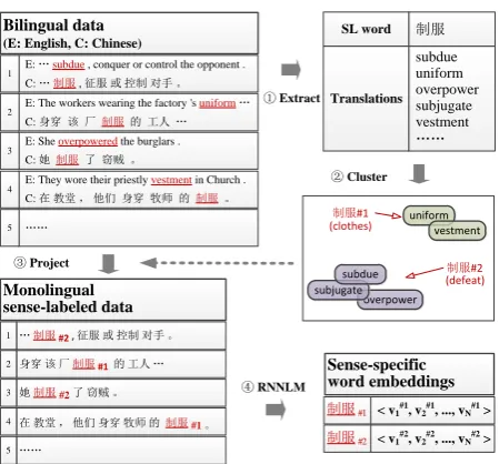
We present a novel and simple method of learning sense-specific word embeddings by using bilingual parallel data. In this method, word sense induction (WSI) is performed prior to the training of NNLMs. We exploit bilingual parallel data for WSI, which is motivated by the intuition that the same word in the
source language with different senses is supposed to have different translations in the foreign language.1
For instance,制服can be translated asinvestment/overpower/subdue/subjugate/uniform, etc. Among
all of these translations,subdue/overpower/subjugateexpress the same sense of制服, whereasuniform
/investmentexpress a different sense. Therefore, we could effectively obtain the senses of one word by clustering its translation words, exhibiting different senses in different clusters.
The created clusters are then projected back into the words in the source language texts, forming a sense-labeled training data. The sense-labeled data are then trained with recurrent neural network langu-gae model (RNNLM) (Mikolov, 2012), a kind of NNLM, to obtain sense-specific word embeddings. As a concrete example, Figure 1 illustrates the process of learning sense-specific embeddings.
∗Email correspondence.
1In this paper,source languagerefers to Chinese, whereasforeign languagerefers to English.
This work is licenced under a Creative Commons Attribution 4.0 International Licence. Page numbers and proceedings footer are added by the organisers. Licence details: http:// creativecommons.org/licenses/by/4.0/
② Cluster
E: The workers wearing the factory 's uniform… C: 身穿 该 厂 制服 的 工人 …
2
E: She overpowered the burglars .
C: 她 制服 了 窃贼 。
3
E: They wore their priestly vestment in Church .
C: 在教堂,他们 身穿 牧师 的 制服 。
Figure 1: An illustration of the proposed method. SL stands forsource language.
To evaluate the sense-specific word embeddings we have learned, we manually construct a Chinese polysemous word similarity dataset that contains 401 pairs of words with human-judged similarities. The performance of our method on this dataset shows that sense-specific embeddings are significantly better in capturing the sense-level similarities for polysemous words.
We also evaluate our embeddings by feeding them as features to the task of Chinese named entity recognition (NER), which is a simple semi-supervised learning mechanism (Turian et al., 2010). In or-der to use sense-specific embeddings as features, we should discriminate the word senses for the NER data first. Therefore, we further develop a novel monolingual word sense disambiguation (WSD) algo-rithm based on the RNNLM we have already trained previously. NER results show that sense-specific embeddings provide noticeable improvements over traditional single embeddings.
Our contribution in this paper is twofold:
• We propose a novel approach of learning sense-specific word embeddings by utilizing bilingual
parallel data (Section 3). Evaluation on a manually constructed polysemous word similarity dataset shows that our approach better captures word similarities (Section 5.2).
• To use the sense-specific embeddings in practical applications, we develop a novel WSD algorithm
for monolingual data based on RNNLM (Section 4). Using the algorithm, we feed the sense-specific embeddings as additional features to NER and achieve significant improvement (Section 5.3).
2 Background: Word Embedding and RNNLM
There has been a line of research on learning word embeddings via NNLMs (Bengio et al., 2003; Mnih and Hinton, 2008; Mikolov et al., 2013b). NNLMs are language models that exploit neural networks to make probabilistic predictions of the next word given preceding words. By training NNLMs, we obtain both high performance language models and word embeddings.
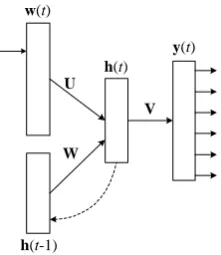
Following Mikolov et al. (2013b), we use the recurrent neural network as the basic framework for train-ing NNLMs. RNNLM has achieved the state-of-the-art performance in language modeltrain-ing (Mikolov, 2012) and learned effective word embeddings for several tasks (Mikolov et al., 2013b). The architecture of RNNLM is shown in Figure 2.
The input layer of RNNLM consists of two components: w(t) andh(t−1). w(t) is theone-hot
representation of the word at time step t,2 h(t−1)is the output of hidden layer at the last time step.
Therefore, the input encodes all previous history when predicting the next word at time stept. Compared
w(t)
y(t)
U
W
V h(t)
h(t-1)
Figure 2: The basic architecture of RNNLM.
with other feed-forward NNLMs, the RNNLM can theoretically represent longer context patterns. The
outputy(t) represents the probability distribution of the next wordp(w(t+ 1)|w(t),h(t−1)). The
output values are computed as follows:
h(t) =f(Uw(t) +Wh(t−1)) (1)
y(t) =g(Vh(t)) (2)
wheref is a sigmoid function andgis a softmax function.
The RNNLM is trained by maximizing the log-likelihood of the training data using stochastic gradi-ent descgradi-ent (SGD), in which back propagation through time (BPTT) is used to efficigradi-ently compute the
gradients. In the RNNLM,Uis the embedding matrix, where each column vector represents a word.
As discussed in Section 1, the RNNLM and even most NNLMs ignore the polysemy phenomenon in natural languages and induce a single embedding for each word. We address this issue and introduce an effective approach for capturing polysemy in the next section.
3 Sense-specific Word Embedding Learning
In our approach, WSI is performed prior to the training of word embeddings. Inspired by Gale et al. (1992) and Chan and Ng (2005), who used bilingual data for automatically generating training examples of WSD, we present a bilingual approach for unsupervised WSI, as shown in Figure 1. First, we extract
the translations of the source language words from bilingual data (¬). Since there may be multiple
translations for the same sense of a source language word, it is straightforward to cluster the translation
words, exhibiting different senses in different clusters ().
Once word senses are effectively induced for each word, we are able to form the sense-labeled training data of RNNLMs by tagging each word occurrence in the source language text with its associated sense
cluster (®). Finally, the sense-tagged corpus is used to train the sense-specific word embeddings in a
standard manner (¯).
3.1 Translation Words Extraction
Given bilingual data after word alignment, we present a way of extracting translation words for source language words by exploiting the translation probability produced by word alignment models (Brown et al., 1993; Och and Ney, 2003; Liang et al., 2006).
More formally, we notate the Chinese sentence as c = (c1, ..., cI) and English sentence as e =
(e1, ..., eJ). The alignment models can be generally factored as:
p(c|e) =Pap(a, c|e) (3)
p(a, c|e) =QJj=1pd(aj|aj−, j)pt(cj|eaj) (4)
where a is the alignment specifying the position of an English word aligned to each Chinese word,
SL Word Translation Words Translation Word Clusters Nearest Neighbours
制服 investment, overpower, subdue, subjugate, uniform
investment,uniform 穿着dress,警服policeman uniform
subdue, subjugate, overpower 打败defeat,击败beat,征服conquer
花 blossom, cost, flower,
spend, take, took
flower, blossom 菜greens,叶leaf,果实fruit
take, cost,spend 花费cost,节省save,剩下rest
法 act, code, France, French, law, method
France, French 德Germany,俄Russia,英Britain
law, act, code 法令ordinance,法案bill,法规rule
method 概念concept,方案scheme,办法way
领导 lead, leader, leadership leader, leadership 主管chief,上司boss,主席chairman lead 监督supervise,决策decision,工作work
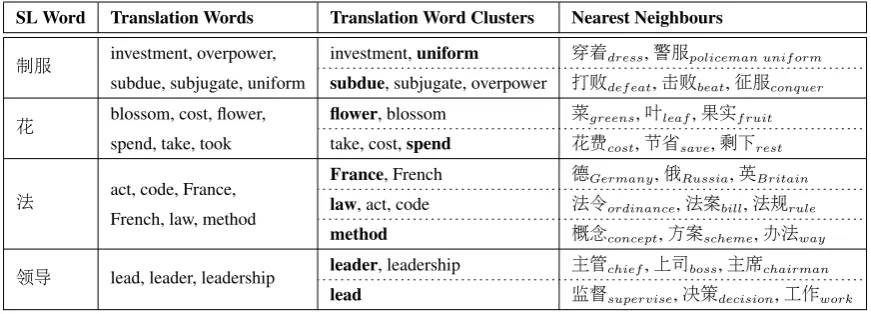
Table 1: Results of our approach on a sample of polysemous words. The second column lists the extracted translation words of the source language word (Section 3.1). The third column lists the clustering results using affinity propagation (Section 3.2). The last column lists the nearest neighbour words computed using the learned sense-specific word embeddings (Section 5.2.2).
In this paper, we use the alignment model proposed by Liang et al. (2006). We utilize the bidirectional
translation probabilities for the extraction of translations, where a foreign language wordwe is
deter-mined as a translation of source language wordwconly if both translation probabilities pt(wc|we) and
pt(we|wc)exceed some threshold0< δ <1.
The second column of Table 1 presents the extraction results on a sample of source language words with the corresponding translation words.
3.2 Clustering of Translation Words
For each source language word, its translation words are then clustered so as to separate different senses. At the clustering time, we first represent each translation word with a feature vector (point), so that we can measure the similarities between points. Then we perform clustering on these feature vectors, representing different senses in different clusters.
Different from Apidianaki (2008) who represents all occurrences of the translation words with their contexts in the foreign language for clustering, we adopt the embeddings of the translation words as
the representations and directly perform clustering on the translation words,3rather than the contexts of
occurrences. The embedding representation is chosen for two reasons: (1) Word embeddings encode rich lexical semantics. They can be directly used to measure word similarities. (2) Embedding representation of the translation words leads to extremely high-efficiency clustering, because the number of translation words is orders of magnitude less than their occurrences.
Moreover, since the number of senses of different source language words is varied, the commonly-used k-means algorithm becomes inappropriate for this situation. Instead, we employ affinity propaga-tion (AP) algorithm (Frey and Dueck, 2007) for clustering. In AP, each cluster is represented by one
of the samples of it, which we call anexemplar. AP finds theexemplarsiteratively based on the
con-cept of “message passing”. AP has the major advantage that the number of the resulting clusters is dynamic, which mainly depends on the distribution of the data. Compared with other possible clustering approaches, such as hierarchical agglomerative clustering (Kartsaklis et al., 2013), AP determines the number of resulting clusters automatically without using any partition criterions.
The third column of Table 1 lists the resulting clusters of the translation words for the sampled pol-ysemous words. We can see that the resulting clusters are meaningful: senses are well represented by clusters of translation words.
3.3 Cross-lingual Word Sense Projection
The produced clusters are then projected back into the source language to identify word senses.
For each occurrencewoof the wordwin the source language corpora, we first select the aligned word
with the highest marginal edge posterior (Liang et al., 2006) as its translation. We then identify the sense
ofwoby computing the similarities of its translation word with eachexemplarof the clusters, and select
the one with the maximum similarity. Whenwois aligned withNULL, we heuristically identify its sense
as the most frequent sense ofwthat appears in the bilingual dataset.
After projecting the word senses into the source language, we obtain a sense-labeled corpus, which is used to train the sense-specific word embeddings with RNNLM. The training process is exactly the same as single embeddings, except that the words in our training corpus has been labeled with senses.
4 Application of Sense-specific Word Embeddings
One of the attractive characteristic of word embeddings is that they can be directly used as word features in various NLP applications, including NER, chunking, etc. Despite of the usefulness of word embed-dings on these applications, previous work seldom concerns that words may have multiple senses, which cannot be effectively represented with single embeddings. In this section, we address this problem by utilizing sense-specific word embeddings.
We take the task of Chinese NER as a case study. Intuitively, word senses are important in NER. For
instance,美is likely to be an NE ofLocationwhen it refers toAmerica. However, when it expresses the
sense ofbeautiful, it should not be an NE.
Using sense-specific word embedding features for NER is not as straightforward as using single em-beddings. For each word in the NER data, we first need to determine the correct word sense of it, which is a typical WSD problem. Then we use the embedding which corresponds to that sense as features. Here we treat WSD as a sequence labeling problem, and solve it with a very natural algorithm based on RNNLM we have already trained (Section 3).
4.1 RNNLM-based Word Sense Disambiguation
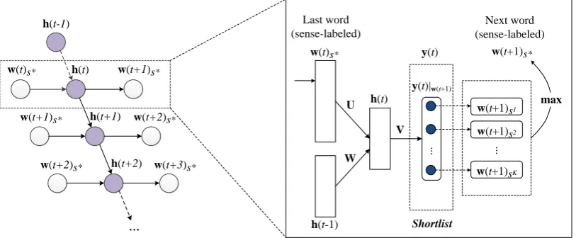
Given the automatically induced word sense inventories and the RNNLM which has already been trained on the sense-labeled data of source language, we first develop a greedy decoding algorithm for the sequential WSD, which works deterministically. Then we improve it using beam search.
Greedy. For wordw, we denote the sense-labeledwaswsk, whereskrepresents thekthsense ofw.
In each step, a single decision is made and the sense of next word (w(t+ 1)) which has the maximum
RNNLM output is chosen, given the current (sense-labeled) wordw(t)s∗ and the hidden layerh(t−1)
at the last time step as input. We simply need to compute a shortlist ofy(t) associated withw(t+ 1),
that is,y(t)|w(t+1)at each step. This process is illustrated in Figure 3.
Beam search. The greedy procedure described above can be improved using a left-to-right beam
search decoding for obtaining a better sequence. The beam-search decoding algorithm keepsBdifferent
sequences of decisions in the agenda, and the sequence with the best overall score is chosen as the final sense sequence.
Note that the dynamic programming decoding (e.g. viterbi) is not applicable here, because of the recurrent characteristic of RNNLM. At each step, decisions made by RNNLM depends on all previous decisions instead of the previous state only, hence markov assumption is not satisfied.
5 Experiments
5.1 Experimental Settings
The Chinese-English parallel datasets we use includeLDC03E24,LDC04E12(1998), theIWSLT 2008
evaluation campaign dataset and thePKU 863parallel dataset. All corpora are sentence-aligned. After
cleaning and filtering the corpus,4we obtain 918,681 pairs of sentences (21.7M words).
In this paper, we useBerkeleyAlignerto produce word alignments over the parallel dataset.5
Berke-leyAligneralso gives translation probabilities and marginal edge posterior probabilities. We adopt the
h(t-1)
Figure 3: Using RNNLM for WSD by sequential labeling (left). Decision at each step of the RNNLM-based WSD algorithm (right).
scikit-learntool (Pedregosa et al., 2011) to implement the AP clustering algorithm.6 The AP algorithm
is not fully automatic in deciding the cluster number. There is a tunable parameter callspreference. A
preferencewith a larger value encourages more clusters to be produced. We set the preferenceat the
median value of the input similarity matrix to obtain a moderate number of clusters. Thernnlmtoolkit
developed by Mikolov et al. (2011) is used to train RNNLM and obtain word embeddings.7 We induce
both single and sense-specific embeddings with 50 dimensions. Finally, We obtain embeddings of a
vocabulary of217K words, with a proportion of8.4%having multiple sense clusters.
5.2 Evaluation on Word Similarity
Word embeddings can be directly used for computing similarities between words, which benefits many practical applications. Therefore, we first evaluate our embeddings using a similarity measurement.
Word similarities are calculated using theMaxSimandAvgSimmetric (Reisinger and Mooney, 2010):
MaxSim(u, v) = max1≤i≤ku,1≤j≤kvs(ui, vj) (5)
standard similarity measure. In this study, we use thecosinesimilarity.
Previous works used the WordSim-353 dataset (Finkelstein et al., 2002) or the Chinese version (Jin and Wu, 2012) for the evaluation of general word similarity. These datasets rarely contain polysemous words, and thus is unsuitable for our evaluation. To the best of our knowledge, no datasets for polysemous word similarity evaluation have been published yet, either in English or Chinese. In order to fill this gap in the research community, we manually construct a Chinese polysemous word similarity dataset.
5.2.1 Chinese Polysemous Word Similarity Dataset Construction
We adopt the HowNet database (Dong and Dong, 2006) in constructing the dataset. HowNet is a Chinese knowledge database that maintains comprehensive semantic definitions for each word in Chinese. The process of the dataset construction includes three steps: (1) Commonly used polysemous words are extracted according to their sense definitions in HowNet. (2) For each polysemous word, we select several other words to form word pairs with it. (3) Each word pair is manually annotated with similarity. In step (1), we mainly took advantage of HowNet for the selection of polysemous words. However, the synsets defined in HowNet are often too fine-grained and many of them are difficult to distinguish,
6scikit-learn.org
particularly for non-experts. Therefore, we manually discard those words with senses that are hard to distinguish.
In step (2), for each polysemous wordw selected in step 1, we sample several other words to form
word pairs withw. The sampled words can be roughly divided into two categories:relatedandunrelated.
Therelatedwords are sampled manually. They can be thehypernym,hyponym,sibling,(near-)synonym,
antonym, ortopically relatedto one sense ofw. Theunrelatedwords are sampled randomly.
In step (3), we ask six graduate students who majored in computational linguistics to assign each word pair a similarity score. Following the setting of WordSim-353, we restrict the similarity score in the range (0.0, 10.0). To address the inconsistency of the annotations, we discard those word pairs with a standard deviation greater than 1.0. We end up with 401 word pairs annotated with acceptable consistency. Unlike the WordSim-353, in which most of the words are nouns, the words in our dataset are more diverse in terms of part-of-speech tags.
Table 2 lists a sample of word pairs with annotated similarities from the dataset. The whole evaluation
dataset will be publicly available for the research community.8
Word Paired word Category Mean.Sim Std.Dev
制服 征服conquer synonym 8.60 0.29
重点key point unrelated 0.12 0.19
出 进enter autonym 7.90 0.97
发表publish near-synonym 7.86 0.76
花 茎plant stem sibling 7.80 0.12
费用cost topic-related 5.86 0.90
面 食物food hypernym 6.50 0.71
Table 2: Sample word pairs of our dataset. The unrelated words are randomly sampled. Mean.Sim
represents the mean similarity of the annotations,Std.Dev represents the standard deviation.
5.2.2 Evaluation Results
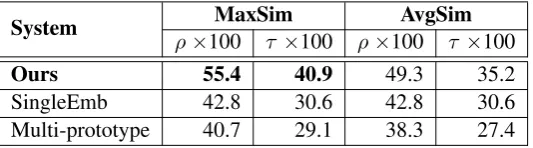
Following Zou et al. (2013), we use Spearman’sρcorrelation and Kendall’sτ correlation for evaluation.
The results are shown in Table 3. By utilizing sense-specific embeddings, our approach significantly
outperforms the single-version using eitherMaxSimorAvgSimmeasurement.
For comparison with multi-prototype methods, we borrow the context-clustering idea from Huang et al. (2012), which was first presented by Sch¨utze (1998). The occurrences of a word are represented by the average embeddings of its context words. Following Huang et al.’s settings, we use a context window
of size 10 and all occurrences of a word are clustered using the spherical k-means algorithm, wherekis
tuned with a development set and finally set to2.
System ρ×100MaxSimτ ×100 ρ×100AvgSimτ ×100
Ours 55.4 40.9 49.3 35.2
SingleEmb 42.8 30.6 42.8 30.6
Multi-prototype 40.7 29.1 38.3 27.4
Table 3: Spearman’sρcorrelation and Kendall’sτ correlation evaluated on the polysemous dataset.
Surprisingly, themulti-prototypemethod performs even slightly worse than the single-version, which
suggests that learning a fixed number of embeddings for every word may even harm the embedding. Additionally, the clustering process of the multi-prototype approach suffers from high memory and time cost, especially for the high-frequency words.
To obtain intuitive insight into the superior performance of sense-specific embeddings, we list in the last column of Table 1 the nearest neighborhoods of the sampled words in the evaluation dataset. The list shows that we are able to find the different meanings of a word by using sense-specific embeddings.
5.3 Application on Chinese NER
We further apply the sense-specific embeddings as features to Chinese NER. We first perform WSD on
the NER data using the algorithm introduced in Section 4. For beam search decoding, the beam sizeB
is tuned on a development set and is finally set to 16.
We conduct our experiments on data fromPeople’s Daily(Jan. and Jun. 1998).9 The original corpus
contains seven NE types.10 In this study, we select the three most common NE types:Person,Location,
Organization. The data from January are chosen as the training set (37,426 sentences). The first 2,000 sentences from June are chosen as the development set and the next 8,000 sentences as the test set.
CRF models are used in our NER system and are optimized by L2-regularized SGD. We use the CRFSuite (Okazaki, 2007) because it accepts feature vectors with numerical values. The state-of-the-art features (Che et al., 2013) are used in our baseline system. For both single and sense-specific embedding features, we use a window size of 4 (two words before and two words after).
5.3.1 Results
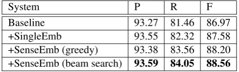
Table 4 demonstrates the performance of NER on the test set. As desired, the single embedding features improve the performance of our baseline, which were also shown in (Turian et al., 2010). Furthermore, the sense-specific embeddings outperform the single word embeddings by nearly 1% F-score (88.56 vs.
87.58), which is statistically significant (p-value<0.01using one-tail t-test).
System P R F
Baseline 93.27 81.46 86.97
+SingleEmb 93.55 82.32 87.58
+SenseEmb (greedy) 93.38 83.56 88.20
+SenseEmb (beam search) 93.59 84.05 88.56
Table 4: Performance of NER on test data.
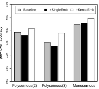
According to our hypothesis, the sense-specific embeddings should bring considerable improvements to the NER of polysemous words. To verify this, we evaluate the per-token accuracy of the polysemous words in the NER test data. We again adopt HowNet to determine the polysemy. Words that are defined with multiple senses are selected as test set. Figure 4 shows that the sense-specific embeddings indeed improve the NE recognition of the polysemous words, whereas the single embeddings even decrease the accuracy slightly. We also obtain improvements on the NE recognition of the monosemous words, which provide evidences that more accurate prediction of polysemous words is beneficial for the prediction of the monosemous words through contextual influence.
6 Related Work
Previous studies have explored the NNLMs, which predict the next word given some history or future words as context within a neural network architecture. Schwenk and Gauvain (2002), Bengio et al. (2003), Mnih and Hinton (2007), and Collobert et al. (2011) proposed language models based on feed-forward neural networks. Mikolov et al. (2010) studied language models based on RNN, which managed to represent longer history information for word-predicting and demonstrated outstanding performance.
Besides, researchers have also explored the word embeddings learned by NNLMs. Collobert et al. (2011) used word embeddings as the input of various NLP tasks, including part-of-speech tagging, chunking, NER, and semantic role labeling. Turian et al. (2010) made a comprehensive comparison of various types of word embeddings as features for NER and chunking. In addition, word embeddings
9www.icl.pku.edu.cn/icl groups/corpus/dwldform1.asp
Polysemous(2) Polysemous(3) Monosemous
per−tok
en accur
acy
0.60
0.65
0.70
0.75
0.80
0.85
0.90
Baseline +SingleEmb +SenseEmb
Figure 4: Per-token accuracy on the polysemous and monosemous words in the NER test data.
Polyse-mous(k) represents the set of words that have more than or equal toksenses defined in HowNet.
are shown to capture many relational similarities, which can be recovered by vector arithmetic in the embedding space (Mikolov et al., 2013b; Fu et al., 2014). Klementiev et al. (2012) and Zou et al. (2013) learned cross-lingual word embeddings by utilizing MT word alignments in bilingual parallel data to constrain translational equivalence.
Most previous NNLMs induce single embedding for each word, ignoring the polysemous property of languages. In an attempt to capture the different senses or usage of a word, Reisinger and Mooney (2010) and Huang et al. (2012) proposed multi-prototype models for inducing multiple embeddings for each word. They did this by clustering the contexts of words. These multi-prototype models simply induced a fixed number of embeddings for every word, regardless of the real sense capacity of the specific word. There has been a lot of work on using bilingual resources for word sense disambiguation (Gale et al., 1992; Chan and Ng, 2005). By using aligned bilingual data along with word sense inventories such as WordNet, training examples for WSD can be automatically gathered. We employ this idea for word sense induction in our study, which is free of any pre-defined word sense thesaurus.
The most similar work to our sense induction method is Apidianaki (2008). They presented a method of sense induction by clustering all occurrences of each word’s translation words. In their approach, occurrences are represented with their contexts. We suggest that clustering contexts suffer from high memory and time cost, as well as data sparsity. In our method, by clustering the embeddings of transla-tion words, we induce word senses much more efficiently.
To evaluate word similarity models, researchers often apply a dataset with human-judged similarities on word pairs, such as WordSim-353 (Finkelstein et al., 2002), MC (Miller and Charles, 1991), RG (Rubenstein and Goodenough, 1965) and Jin and Wu (2012). For context-based multi-prototype mod-els, (Huang et al., 2012) constructs a dataset with context-dependent word similarity. To the best of our knowledge, there is no publicly available datasets for context-unaware polysemous word similarity evaluation yet. This paper fills this gap.
7 Conclusion
This paper presents a novel and effective approach of producing sense-specific word embeddings by exploiting bilingual parallel data. The proposed embeddings are expected to capture the multiple senses of polysemous words. Evaluation on a manually annotated Chinese polysemous word similarity dataset shows that the sense-specific embeddings significantly outperforms the single embeddings and the multi-prototype approach.
Acknowledgments
We are grateful to Dr. Zhenghua Li, Yue Zhang, Shiqi Zhao, Meishan Zhang and the anonymous review-ers for their insightful comments and suggestions. This work was supported by the National Key Basic Research Program of China via grant 2014CB340503 and 2014CB340505, the National Natural Science Foundation of China (NSFC) via grant 61370164.
References
Marianna Apidianaki. 2008. Translation-oriented word sense induction based on parallel corpora. InIn Proceed-ings of the 6th Conference on Language Resources and Evaluation (LREC), Marrakech, Morocco.
Yoshua Bengio, R´ejean Ducharme, Pascal Vincent, and Christian Janvin. 2003. A neural probabilistic language model. The Journal of Machine Learning Research, 3:1137–1155.
Peter F Brown, Vincent J Della Pietra, Stephen A Della Pietra, and Robert L Mercer. 1993. The mathematics of statistical machine translation: Parameter estimation.Computational linguistics, 19(2):263–311.
Yee Seng Chan and Hwee Tou Ng. 2005. Scaling up word sense disambiguation via parallel texts. InAAAI, volume 5, pages 1037–1042.
Wanxiang Che, Mengqiu Wang, Christopher D. Manning, and Ting Liu. 2013. Named entity recognition with bilingual constraints. InProceedings of the 2013 Conference of the North American Chapter of the Association for Computational Linguistics: Human Language Technologies, pages 52–62, Atlanta, Georgia, June.
Ronan Collobert, Jason Weston, L´eon Bottou, Michael Karlen, Koray Kavukcuoglu, and Pavel Kuksa. 2011. Natural language processing (almost) from scratch.The Journal of Machine Learning Research, 12:2493–2537. Zhendong Dong and Qiang Dong. 2006.HowNet and the Computation of Meaning. World Scientific.
Lev Finkelstein, Evgeniy Gabrilovich, Yossi Matias, Ehud Rivlin, Zach Solan, Gadi Wolfman, and Eytan Ruppin. 2002. Placing search in context: The concept revisited.ACM Transactions on Information Systems, 20(1):116– 131.
Brendan J Frey and Delbert Dueck. 2007. Clustering by passing messages between data points. science, 315(5814):972–976.
Ruiji Fu, Jiang Guo, Bing Qin, Wanxiang Che, Haifeng Wang, and Ting Liu. 2014. Learning semantic hierar-chies via word embeddings. InProceedings of the 52th Annual Meeting of the Association for Computational Linguistics: Long Papers-Volume 1, Baltimore MD, USA.
William A Gale, Kenneth W Church, and David Yarowsky. 1992. Using bilingual materials to develop word sense disambiguation methods. InProceedings of the 4th International Conference on Theoretical and Methodologi-cal Issues in Machine Translation, pages 101–112.
Eric H Huang, Richard Socher, Christopher D Manning, and Andrew Y Ng. 2012. Improving word representations via global context and multiple word prototypes. InProceedings of the 50th Annual Meeting of the Association for Computational Linguistics: Long Papers-Volume 1, pages 873–882.
Peng Jin and Yunfang Wu. 2012. Semeval-2012 task 4: evaluating chinese word similarity. InProceedings of the First Joint Conference on Lexical and Computational Semantics-Volume 1: Proceedings of the main conference and the shared task, and Volume 2: Proceedings of the Sixth International Workshop on Semantic Evaluation, pages 374–377.
Dimitri Kartsaklis, Mehrnoosh Sadrzadeh, and Stephen Pulman. 2013. Separating disambiguation from composi-tion in distribucomposi-tional semantics. CoNLL-2013, pages 114–123.
Alexandre Klementiev, Ivan Titov, and Binod Bhattarai. 2012. Inducing crosslingual distributed representations of words. InProceedings of COLING 2012, pages 1459–1474, Mumbai, India, December.
Percy Liang, Ben Taskar, and Dan Klein. 2006. Alignment by agreement. InProceedings of the main conference on Human Language Technology Conference of the North American Chapter of the Association of Computa-tional Linguistics, pages 104–111.
Tomas Mikolov, Stefan Kombrink, Anoop Deoras, Lukar Burget, and J ˇCernock`y. 2011. Rnnlm-recurrent neural network language modeling toolkit. InProc. of the 2011 ASRU Workshop, pages 196–201.
Tomas Mikolov, Kai Chen, Greg Corrado, and Jeffrey Dean. 2013a. Efficient estimation of word representations in vector space. arXiv preprint arXiv:1301.3781.
Tomas Mikolov, Wen-tau Yih, and Geoffrey Zweig. 2013b. Linguistic regularities in continuous space word representations. InProceedings of NAACL-HLT, pages 746–751.
Tomas Mikolov. 2012.Statistical Language Models Based on Neural Networks. Ph.D. thesis, Ph. D. thesis, Brno University of Technology.
George A Miller and Walter G Charles. 1991. Contextual correlates of semantic similarity. Language and cognitive processes, 6(1):1–28.
Andriy Mnih and Geoffrey Hinton. 2007. Three new graphical models for statistical language modelling. In
Proceedings of the 24th international conference on Machine learning, pages 641–648.
Andriy Mnih and Geoffrey E Hinton. 2008. A scalable hierarchical distributed language model. InAdvances in neural information processing systems, pages 1081–1088.
Franz Josef Och and Hermann Ney. 2003. A systematic comparison of various statistical alignment models.
Computational linguistics, 29(1):19–51.
Naoaki Okazaki. 2007. Crfsuite: a fast implementation of conditional random fields (crfs). URL http://www. chokkan. org/software/crfsuite.
F. Pedregosa, G. Varoquaux, A. Gramfort, V. Michel, B. Thirion, O. Grisel, M. Blondel, P. Prettenhofer, R. Weiss, V. Dubourg, J. Vanderplas, A. Passos, D. Cournapeau, M. Brucher, M. Perrot, and E. Duchesnay. 2011. Scikit-learn: Machine learning in Python. Journal of Machine Learning Research, 12:2825–2830.
Joseph Reisinger and Raymond J Mooney. 2010. Multi-prototype vector-space models of word meaning. In
Human Language Technologies: The 2010 Annual Conference of the North American Chapter of the Association for Computational Linguistics, pages 109–117.
Herbert Rubenstein and John B Goodenough. 1965. Contextual correlates of synonymy. Communications of the ACM, 8(10):627–633.
Hinrich Sch¨utze. 1998. Automatic word sense discrimination. Computational linguistics, 24(1):97–123.
Holger Schwenk and Jean-Luc Gauvain. 2002. Connectionist language modeling for large vocabulary continuous speech recognition. InAcoustics, Speech, and Signal Processing (ICASSP), 2002 IEEE International Confer-ence on, volume 1, pages 765–768.
Richard Socher, Eric H Huang, Jeffrey Pennin, Christopher D Manning, and Andrew Ng. 2011. Dynamic pooling and unfolding recursive autoencoders for paraphrase detection. InAdvances in Neural Information Processing Systems, pages 801–809.
Joseph Turian, Lev Ratinov, and Yoshua Bengio. 2010. Word representations: a simple and general method for semi-supervised learning. In Proceedings of the 48th Annual Meeting of the Association for Computational Linguistics, pages 384–394.
Mo Yu, Tiejun Zhao, Daxiang Dong, Hao Tian, and Dianhai Yu. 2013. Compound embedding features for semi-supervised learning. InProceedings of NAACL-HLT, pages 563–568.