Mining Words in the Minds of Second Language Learners: Learner Specific Word Difficulty

Mining words in the minds of second language learners:

learner-specific word difficulty

Yo Ehara

_{Issei Sato}

_{Hidekazu Oiwa}

_{Hiroshi N akagawa}

(2) JSPS Research Fellow, Tokyo, Japan

(3) Information Technology Center, the University of Tokyo, Tokyo, Japan

④❡❤❛r❛✱s❛t♦✱♦✐✇❛⑥❅r✳❞❧✳✐t❝✳✉✲t♦❦②♦✳❛❝✳❥♣✱ ♥❛❦❛❣❛✇❛❅❞❧✳✐t❝✳✉✲t♦❦②♦✳❛❝✳❥♣

A

1 Introduction

When learning second languages, vocabulary knowledge is as important as, or sometimes more important, than grammar. The importance of vocabulary knowledge has been a main focus in the last decade in the field of second language acquisition (SLA).

Studies regarding vocabulary knowledge of second language learners have been mainly focusing on two major tasks: devising methods for measuring the size of the second language vocabulary of learners for testing purposes (Schmitt et al., 2001; Laufer and Nation, 1999; Nation, 1990) and determining the words that the learnersshouldlearn (Nation, 2006). However, there have been few studies on what kind of words learnersactuallyknow. This is the basic research question for our research.

To study what words second language learners actually know, we focused on thevocabulary predictiontask. In this task, we aim to build a model that predicts, given a word and a learner, whether or not the learner knows the word. As far as we know, Ehara et al. (2010) is the only study that dealt directly with the vocabulary prediction task. They applied this task to a reading support user interface for second language learners that automatically identifies the words unfamiliar to the learner on a Web page.

The vocabulary prediction task is important for both theory and application. From the theoretical point of view, this task is interesting in that it mines the words second language learners know and creates a model on what kinds of words learners actually know. From the model, we can interpret the patterns or tendency of the learners’ process of memorizing second language words. Studying the vocabulary prediction task may also lead to determining if learners actually learn words that SLA experts recommend.

From the application point of view, this task can be used in user-adaptation for reading and writing applications to support second language learners. Ehara et al. (2010)’s model is of this type. They successfully showed the effectiveness of their system. With the increase in Web-based language learning environments, possible data sources for learners’ vocabulary knowledge are also increasing. Studying the vocabulary prediction task can shed light on these data sources, and they can be used to further understand the vocabulary knowledge of second language learners.

By using machine learning terminology, the vocabulary prediction task can be categorized as a binary classification task: given a word and a learner, it predicts whether or not the learner knows the word. Therefore, a number of machine learning methods, such as a support vector machine (SVM) for the binary classification task, can be used as predictors. However, to answer our research question, what kind of words learnersactuallyknow, we want predictors to be able to do more than just predict. Rather, we want predictors that are practical and useful for analysis. Specifically, we list the following properties we want predictors to have.

interpretable weight vector Most predictors use weight vectors trained with data. Weight vectors of some models can be interpreted as quantitative measures of word difficulty and learner ability. Interpretable weight vectors are essential for analysis to find the patterns or tendency of learners’ process of memorization, and to further understand the basic research question: what kind of words do second language learners actually know? out-of-sample Settings in the vocabulary prediction task can be divided into two for handling

words, i.e., there is at least one training dataset for all the words appearing in the test data. This can be seen as filling in the blanks of a learner-word matrix. In contrast, theout-of-samplesetting support new words, i.e., some or all words in the test data are missing in the training data. To create the training data, we need to ask learners whether or not they know the words. Thus, creation of the training data is very financially costly and burdensome for learners. In a realistic setting, we can ask learners about only a small subset of words, and the predictors usually have to predict all the rest. The out-of-sample setting is more difficult but more realistic than the in-matrix setting.

learner-specific word difficulty This is the core beneficial property of the proposed model. Some interpretable weight vectors can determine word difficulty. However, the perceived difficulty of a word differs from learner to learner. For example, a learner interested in music may know music-related words that even high-level learners may not be familiar with. For another example, suppose that normally difficult words are used in the names of well known commercial products and services. In this case, again, low-ability learners may know these words through the product names. Thus, it is preferable for a model to be able to detect this kind of learner specialty.

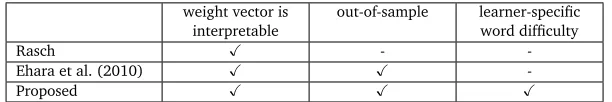
weight vector is interpretable

out-of-sample learner-specific word difficulty

Rasch Ø -

-Ehara et al. (2010) Ø Ø

-Proposed Ø Ø Ø

Table 1: Properties of models. The proposed model supports all preferred properties. Ordinary binary classifiers only can classify: their weight vectors are not interpretable asword difficulty

andlearner abilityas those of the other models listed here.

Table 1 summarizes the models explained in this paper. We can see that only the proposed model supports all the properties. Although ordinary binary classifiers, such as SVMs, can be used for the vocabulary prediction task, their weight vectors cannot be used to determine word difficulty and learner ability that we want for analysis. Thus, we ruled out typical binary classifiers.

The structure of this paper is as follows. We first focus on extending the basic interpretable model: the Rasch model (Rasch, 1960; Baker and Kim, 2004). Although the Rasch model lacks many of the preferred properties, it provides a rough idea for the vocabulary prediction task. To explain why the Rasch model lacks many of these properties, we then introducethe general formof the likelihood of the Rasch model. This generalization provides a way of supporting the preferred properties. Through this generalization, we can derive the Rasch model, the model proposed by Ehara et al. (2010), and the proposed model.

The contributions of this paper are as follows:

•We introduce the general form of likelihood of the Rasch model that can explain the reason this model lacks the desired properties.

•We propose a model that supports all desired properties using this general form. •In an evaluation, our model successfully detected the specialties of second language

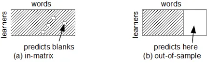
Figure 1: Two problem settings; (a) in-matrix, (b) out-of-sample.

2 Problem setting

LetUbe a set of learners, andVbe a set of vocabulary. We denote the number of learners as|U|and the number of words as|V|. A datum can be expressed using the triplet(y,u,v). Here,y∈ {0, 1}is the label denoting whether or not learneruknows wordv,(1,u,v)means that learneruknows wordv, and(0,u,v)means he/she does not know wordv. Using these notations, the vocabulary prediction task is defined to predict the label y given(u,v). We denote a dataset ofNdata asD={(y1,u1,v1), . . . ,(yN,uN,vN)}.

For simplicity, we assume that for one learneru∈Uand wordv∈Vpair, there exists only one labely. This restriction enables us to depict the data set in a matrix form, as shown in Figure 1. The rows of the matrix correspond to learners and the columns of the matrix correspond to words. Under this assumption, for one row (learner) and one column (word), there is only one cell; thus, only one labely. With this restriction,Nis the number of cells in the matrix. The dataset we used in the evaluation agrees with this restriction; however, we cannot always assume this restriction in a realistic setting. This is the reason we did not directly jump to matrix-based prediction methods such as low-rank approximation using singular value decomposition. For example, in a realistic dataset, such as word-click logs in a reading support system, contradiction and repetition are common. For contradiction, if both(1,u,v)and(0,u,v) appear in the dataset, it may mean these two datasets are unreliable. Repetition of multiple (1,u,v)may mean that learneruis more familiar with wordvthan just one(1,u,v). All the models that we explain in the later sections of this paper can handle these cases.

Figure 1 explains thein-matrixandout-of-samplesettings. The hashed areas denote the training data, and the blank areas denote the test data. In thein-matrixsetting, the test data are randomly placed in the matrix.

3 Rasch model

Although the vocabulary prediction task is quite novel, there have been a substantial amount of work in SLA about which words a learnershouldlearn first. Many studies recommend learners to learn words according to word frequency in general corpora because word frequency can be used as a rough measure of word difficulty. Of course, the learner does not necessarily learn the words in this recommended order. As stated in the introduction, it is one of our research questions to check if learnersactuallylearn in this order.

1. We rank words according to a measure of word difficulty. 2. We decide the threshold for a learner.

3. Words with greater difficulty than the threshold are predicted to be unfamiliar to the learner, and vice versa.

Although this model seems too simple, it is the core idea of the Rasch model, which has been widely used in language testing.

Figure 2: Simple vocabulary prediction model. (a) First, assume there is a difficulty measure that maps each word to a point on the axis of the measure. (b) Second, each learner’s ability is also mapped to a point on the same axis. (c) Third, the words with the greatest difficulty to the point designating the learner’s ability is predicted to be unfamiliar to the learner, and vice versa. Given learneruand wordv, the Rasch model models the probability of learneruknowing word

vas follows:

P y=1|u,v=σ au−dv, (1) whereσ(t) = 1+exp(−t)−1denotes the logistic sigmoid function. There are two kinds of parameters to be trained:

dv the difficulty of wordv,

au the ability of learneru.

In the Rasch model, the subtraction of two parametersau−dvin Eq. (1) denotes exactly the same mechanism as the simple vocabulary prediction in Figure 2. Here,dvmaps each wordv into a point on the axis, andauworks as a threshold. WhenP(y=1|u,v)≥0.5, we can assume learneruknows wordv. Due to the logistic sigmoid function,P(y=1|u,v)≥0.5 holds true if and only ifau−dv≥0, that is,au≥dv. Therefore, the Rasch model determines that learneru knows all words whose word difficultydvis lower than the learners’ abilityau. Note that not only the ability of learneraubut also the difficulty of worddvis estimated from the data in the Rasch model.

The priors for the parameters are usually set as follows:

P au|ηa = N €

0,η−1_a Š (∀u∈U), (2)

P dv|ηd = N €

whereN denotes the probability distribution function of the normal distribution. Frequently, the hyper parametersηaandηdare set asηa=ηd. Ifηa=ηd, the parameters,dvandauof the Rasch model can be obtained using a standard log-linear model solver.

One of the notable problems with the Rasch model is that it does not take into account the

out-of-samplesetting. That is, it cannot predict words that do not appear in the training set. For example, if there is a new word in a document in a reading support system, we need to re-create the training set with the new word for the system to be able to predict that word as well. This restriction makes the application systems using the vocabulary prediction task impractical.

4 General form of likelihood

In the previous section, we stated that the Rasch model does work under the out-of-sample setting, which frequently occurs in a realistic setting. This section attempts to locate the fundamental reason the out-of-sample problem arises by generalizing the likelihood of the Rasch model.

Let us discuss the difficulty parameterdvof the Rasch model from another perspective. If we define a function asf(v) =dv, we can understand thatdvis a function that takes wordvas its argument and returns the difficulty of wordv. This means that we do not need to allocate the number of variables|V|to determine the difficulty of a word as the Rasch model does. Instead, all that we need is a function that returns word difficulty for given wordv.

We can further extendf to be the formf(u,v): a function that takes learneruand wordvas its argument and returns the difficulty of wordvfor learneru. By usingf(u,v), we can generalize the likelihood function of the Rasch model as follows:

P y=1|u,v=σ au−f(u,v). (4) The Rasch model is a special version of Eq. (4) where we setf(u,v) =dv. We can see that the fundamental cause of the out-of-sample problem in the Rasch model comes from this poorly designed f. There is a 1-to-1 mapping between parameters and words in this design off. Therefore, if some words are missing in the training set, parameters arise that are not trained. Note that Eq. (4) generalizes only the likelihood of the Rasch model. Of course, to fully define a model, we must define priors as well. Moreover, the priors must be designed carefully; otherwise, a model can produce poor results regardless of the design off.

One may think of extending the learner ability parameterau to be a function as well. Of course, we can do this extension in theory. However, unlike word difficulty parameters, little information is practically available for learners. Therefore, it is preferable for a model to require as little information from learners as possible. Since the complex design off may require much information, we kept the learner ability parameterausimple.

4.1 Shared difficulty model

Even if there is a new word in the test data and there are words in the training data that share the same features with the new word, the word difficulty of the new word can be obtained by calculatingw⊤_{φ(v). The full form of the likelihood becomes the following.}

P y=1|u,v;w=σ€au−w⊤φ(v) Š

. (5)

Priors for the likelihood Eq. (5) are set as follows. We call this model the shared difficulty model.

P au|ηa = N €

0,η−_a1Š (∀u∈U), (6)

P w|ηw = N €

0,η−_w1IŠ, (7)

whereIdenotes theK×K-sized identity matrix. If we setη_w=η_a, this model reduces to a simple l2-norm-regularized logistic regression as Ehara et al. (2010) used. However, they did not mention the out-of-sample setting or the general likelihood.

5 Proposed model

One problem in both the Rasch and shared difficulty models is that all learners share a single word difficulty measure. This means that the same ranking of a word is shared by all the learners, e.g., the word “tremble” is more difficult thanworshipaccording to all the learners. Thus, the Rasch and shared difficulty models cannot take into account a leaner’s specialty. In reality, it is common that even low-ability learners know difficult words with the help of their interests in a specific topic. For example, learners who are interested in music are likely to have a large vocabulary of music-related words in second languages regardless of the difficulty of the words. Modeling this kind of learner specialty is essential in designing user-adaptive supports for second language learners.

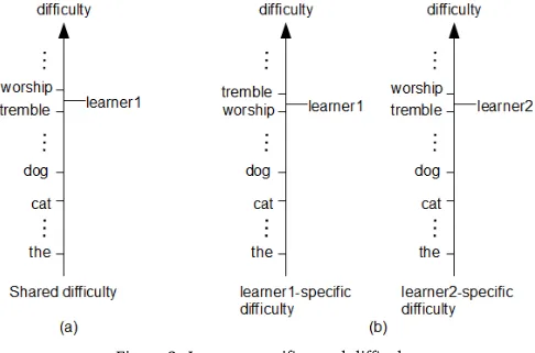
Figure 3: Learner-specific word difficulty.

Name Design off Priors Notes

Rasch f(u,v) =dv

P au|ηa=N €

0,η−1_a Š

P dv|ηd=N €

0,η−_d1Š

-Shared diffi-culty model (Ehara et al., 2010)

f(u,v) =w⊤_φ(v) P au|ηa=N €

0,η−_a1Š

P w|ηw=N €

0,η−_w1IŠ

Reduced to Rasch model if φ(v) is 1-dimensional and

φ(v) =1.

Proposed f(u,v) =w⊤

uφ(v) P au|ηa

=N€0,η−1_a Š

P w0=N €

0,η−1_w IŠ

P wu|w0=N €

w0,λ−1I Š

Reduced to the shared difficulty model if we set wu=w0 (∀u∈U). Table 2: Summary of models explained so far. The Rasch model is a special case of the shared difficulty model, and the shared difficulty model is a special case of the proposed model.

right side of the axis, learner thresholds are plotted according to the learners’ ability parameters

au. The predictor determines that a learner does not know all the words above his/her threshold. In Figure 3 (a), all three learners share the same word difficulty. Therefore, the model cannot represent a learner who knows the word “worship” but does not know the word “tremble”. This problem can be solved by introducing a difficulty axis for every learner as Figure 3 (b) does. In (b), “learner 1” is modeled as knowing the word “worship” but not the word “tremble”, while “learner 2” is modeled as knowing the word “tremble” but not the word “worship”. This kind of flexible modeling is impossible in the Rasch and shared difficulty models.

With the general model explained above, we can easily explain the fundamental cause of this problem: in the current models, f(u,v)depends only onv, and does not depend onu. Therefore, tackling this problem is simple: letf(u,v)depend onuas well. In the proposed model, we definef(u,v) =w⊤

uφ(v). The full form of the likelihood is shown as follows.

P y=1|u,v;wu=σ €

au−w⊤uφ(v) Š

. (8)

This likelihood has far more parameters to be trained than the current models. Since the dimension size of the feature space isK,wuis aK-dimension vector. Since we have|U|learners, we haveK|U|parameters to tune in total. Priors must be carefully designed to tune this large number of parameters. We designed the priors as follows:

P au|ηa = N €

0,η−1_a Š (∀u∈U), (9)

P w0 = N €

0,η−_w1IŠ, (10)

P wu|w0 = N €

w0,λ−1I Š

. (11)

6 Estimation of model parameters

This section describes methods for estimating the model parameters. We use maximum-a-posteriori (MAP) estimation for all three models: Rasch, shared difficulty, and proposed. As we explained, the shared difficulty and Rasch models are special cases of the proposed model. Therefore, we first explain the optimization of the proposed model.

The negative log of the negative log posterior of the proposed model takes the following form:

l W,a,w0 = N X

i=1

nll yi,ui,vi+

λ

2 X

u∈U wu−w0

2

(12)

+ η₂ww02+η₂aX u∈U

a2

u . (13)

We define the negative log likelihood function of the proposed model asnll y,u,v def= log€1+exp€−y€au−w⊤uφ(v)

ŠŠŠ

. We define Wandaas follows for concise notation: W={wu|∀u∈U},a ={au|∀u∈U}. This functionl W,a,w0is convex (Kajino et al., 2012) over all the variablesW,a,w0. Thus, the MAP model parametersW,ˆ ˆa, andwˆ0can be estimated by minimizingl W,a,w0w.r.t.W,a, andw0.

Based on Kajino et al. (2012), we minimizel W,a,w0iteratively as follows:

minimizing w.r.t. W, a We fixw0 and minimizel W,a,w0w.r.t. Wanda. Kajino et al. (2012) used the Newton method for this optimization. Using the Newton method requires

O(K2)memory, whereKis the dimension ofwuandw0. This is problematic whenK

increases. To tackle this problem, we used L-BFGS (Liu and Nocedal, 1989), which requires onlyO(K)memory, for this optimization instead. Specifically, we used the library liblbfgs (Okazaki, 2007).

minimizing w.r.t. w0 We fixWandato minimizel w.r.t. w0. This minimization can be achieved analytically as follows:

w0=

λ ηw+|U|λ

X

u∈U

wu . (14)

We repeated these two minimizations iteratively until convergence.

Both the Rasch and shared difficulty models are special cases of the proposed model when wu=w0 (∀u∈U). This means that the second minimization is unnecessary for the Rasch and shared difficulty models. Thus, the parameters, i.e., the weight vector, of the Rasch and shared difficulty models can be obtained by simply performing the first minimization.

7 Evaluation

7.1 Dataset

Corpus name Type of English Size (in token) Description British National

Cor-pus (BNC) (The BNC Consortium, 2007)

British 100 mil. General corpus

The Corpus of Con-temporary American English (COCA) (Davies, 2011)

American 450 mil. General corpus

Open American National Corpus (OANC) (Ide and Suderman, 2007)

American 14 mil. General corpus

Brown corpus (Fran-cis and Kucera, 1979)

American 1 mil. General corpus

Google 1-gram (Brants and Franz, 2006)

Mixed 1,024,948 mil. Huge, but not gen-eral

Table 3: Feature sources.

This dataset was designed to be quite exhaustive. Every learner was handed a randomly sorted questionnaire comprising 12, 000 words and asked to answer how well he/she knew the words in the questionnaire based on a five-point scale. We regarded level 5 as onlyy=1; the learner knows the word. Otherwise we regardedy=0; the learner does not know the word. Out of the 12, 000 words, 1 word was a pseudo-word, i.e., it looks like an English word but actually is not. Fifteen learners were paid, and 1 learner was not. Since we found that the unpaid learner’s data were too noisy, we used only the data of the 15 paid learners. We had|V|=11, 999 words × |U|=15 learners; 179, 985 data points in total.

The negative log of the 1-gram probabilities of each word in each corpus is used as features for training. The collected corpora for feature sources are compiled in Table 3. Ehara et al. (2010) used one large corpus, Google-1gram. However, from the perspective of SLA, it is typically not justified because it is not a general corpus; thus, its frequencies could be biased. To avoid being biased, we collected many general corpora and used them as features.

When training, hyper parameters were chosen by grid search and 5-fold cross validation within the training set. The set of hyper parameters that performed best in this cross validation was selected. Then, we trained the model with all the training sets using the selected hyper parameters. We then applied the model to the test set to obtain the results. For the Rasch and shared difficulty models, each hyper parameter,ηd,ηa, andηw, was chosen by grid search from {0.01, 2−3_{, 2}−2_{, 2}−1_{, 1.0, 2}1_{, 2}2_{, 2}4_{}. For the proposed model, each hyper parameter,η}

a,ηw, and

λ, was chosen by grid search from{2−2_{, 2}−1_{, 1.0, 2}1_{, 2}2_}.

7.2 Evaluation of learner-specificity

For a measure of learner-specificity, we introduce thevarianceof learner-specific word difficulty. In the proposed model, the learner-specific difficultyf(u,v)of wordvfor learneruis defined as

f(u,v) =w⊤

uφ(v). Unlike the current models that assign single word difficulty for all learners, we can naturally define the variance of word difficulty over learners. Given the set of estimated weight vectors for all|U|learners,{wuˆ |u∈U}, for wordv∈V, we defineM ean(v)andVar(v) as follows:

M ean(v) def= 1 |U|

X

u∈U

f(u,v) = 1 |U|

X

u∈U ˆ w⊤

uφ(v), (15)

Var(v) def= 1 |U|

X

u∈U

f(u,v)−M ean(v)2= 1 |U|

X

u∈U €

ˆ w⊤

uφ(v)−M ean(v) Š2

. (16)

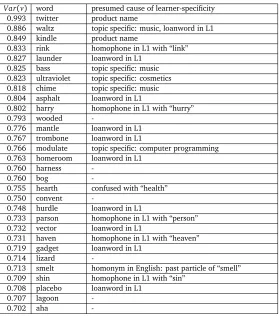
Table 4 lists the words with largest variancesVar(v)in descending order.Var(v)increases when some low-ability learners know the words and some high-ability learners do not. In other words, it increases when low-ability learners know the word for some reason other than the easiness of the word, and vice versa. Table 4 is constructed from the weight vectors of the proposed model. The weight vectors are trained in the in-matrix setting. Out of 179, 985 data points, 177, 985 were used for training. Features and hyper parameter tuning are explained in §7.1. 2, 000 data points were used to check the accuracy, which was 83.40%.

For example, it is very interesting and noteworthy that the word “twitter” comes at the top of the list of Table 4. This is presumably due to the famous micro-blogging service, Twitter. The word “twitter” itself is a rare word. For example, in the British National Corpus, the frequency of the word “twitter” is merely 17 while the word “the” is 6, 043, 900. The words whose frequency is the same with the word “twitter” are: “abet”, “beguile”, and “coddle”. Since these three words are in the dataset as well, the rareness of words only cannot explain the large variance of the word “twitter”. This dataset was created in Japan in January 2009 when Twitter was not as predominant as it is today. Therefore, some low-level learners knew the word “twitter” through the name of the service while some high-level learners did not. Additionally, Table 4 ranks another similar example at the third: “kindle”. The first Amazon Kindle was released in the United States in 2007.

Likewise, we annotated presumable reasonsVar(v)increased in the rightmost column of Table 4. Although these reasons are speculation, it is difficult to find the correct reason learners know a word, even for learners themselves, because we usually do not remember how we learned foreign words. Our speculations are intuitive and understandable for Japanese-native English as a Second Language (ESL) learners.

Product name The words “twitter” and “kindle” correspond to this case. When a difficult word is used as the name of a famous product, it is possible that even low-ability learners would know the word through the name of the product, which makes the variance larger. Loanwords in L1Some words in the second language are borrowed by the learners’ native

Var(v) word presumed cause of learner-specificity 0.993 twitter product name

0.886 waltz topic specific: music, loanword in L1 0.849 kindle product name

0.833 rink homophone in L1 with “link” 0.827 launder loanword in L1

0.825 bass topic specific: music 0.823 ultraviolet topic specific: cosmetics 0.818 chime topic specific: music 0.804 asphalt loanword in L1

0.802 harry homophone in L1 with “hurry” 0.793 wooded

-0.776 mantle loanword in L1 0.767 trombone loanword in L1

0.766 modulate topic specific: computer programming 0.763 homeroom loanword in L1

0.760 harness

-0.760 bog

-0.755 hearth confused with “health” 0.750 convent

-0.748 hurdle loanword in L1

0.733 parson homophone in L1 with “person” 0.732 vector loanword in L1

0.731 haven homophone in L1 with “heaven” 0.719 gadget loanword in L1

0.714 lizard

-0.713 smelt homonym in English: past particle of “smell” 0.709 shin homophone in L1 with “sin”

0.708 placebo loanword in L1 0.707 lagoon

-0.702 aha

-Table 4: Top 30 words with largest variancesVar(v)in descending order. LargeVar(v)suggests large learner-specificity. Japanese is the native language (L1) of this dataset.

perceive the meaning of the word through its corresponding loanword in L1, which makes the variance larger.

Homophones in L1 If there are two words that are homophones in the learners’ native lan-guage, and one of the two words is easier than the other, a low-ability learner may mistake the difficult one for the easy one. For example, a large variance of the word “rink” is caused by low-ability learners’ mistake for the word “link” because the Japanese language does not distinguish “l” and “r”. For example, Japanese has no distinction between “par” and “per”, the large variance of the word “parson” is presumably due to some learners mistaking this word for the word “person”.

Homonyms in English“smelt” is a verb that means extracting metals by heat. Yet, it is also the past participle of the word “smell”. Although the conjugated forms were removed from this dataset, some low-ability learners presumably did not notice it and thought that they were asked if they knew the word “smelt” as the past participle of the word “smell”. Some high-ability learners presumably knew that the word “smelt” has a meaning other than the past participle of “smell” and not asked about “smelt” as the past participle. If they did not know what was the meaning other than the past participle of “smell”, they answered no in the dataset.

Note that the variance of the learners’ responseyfor a word in the raw datacannotproduce an interesting listing as in Table 4 becauseyis binary, 0 or 1. It trivially lists words of which half the learners in the dataset know. For example, if there are 15 learners in a data set, it is trivial to determine the words with the highest variance ofyas those that 8 learners knew and 7 learners did not, or 7 learners knew and 8 learners did not. This means that many words have the highestyvariance. In this dataset, 1, 408 of 11, 999 words had the highestyvariance. Therefore,yvariance does not produce any interesting results.

In contrast to Table 4, the words with smallestVar(v)are trivial. They are words all the learners knew or all the learners did not know. The 30 words with the smallest variances were: am, beach, doll, during, eastern, equal, excellent, green, handwriting, hungry, important, logic, love, luck, marine, paradise, shop, technical, writing, pet, unknown, loose, maker, acquittal, arduous, cot, exchequer, hindsight, innuendo, and purr.

Finally, we investigated the accuracy in the out-of-sample setting. We split the 11, 999 words into 2, 000 words for the test set and the rest for the training set. The size of training data was 149, 985 and the size of test data was 30, 000. Hyper parameter tuning and feature set were the same as we stated in §7.1. The Rasch model achieved 66.32%, the shared difficulty model (Ehara et al., 2010) achieved 77.67%, and the proposed model achieved 77.81%.

8 Related Work

The proposed model is mathematically very similar to those proposed by Evgeniou and Pontil (2004) and Kajino et al. (2012). However, these models are for totally different purposes than ours: Evgeniou and Pontil (2004) aimed at multi-task learning and Kajino et al. (2012) aimed at crowd-sourcing. As the Rasch model is rarely used for these purposes, they did not mention the relationship between the Rasch and proposed models, let alone the generalization of the likelihood of the Rasch model. Strictly speaking, these two models differ from our model in that they do not include the Rasch and shared difficulty models (Ehara et al., 2010) as special cases while our proposed model does.

We extended word difficulty to learner-specific word difficulty by focusing on the analysis of the vocabulary knowledge of adult second language learners. Aside from second languages, study of vocabulary knowledge is also important for the analysis of child development in terms of native language. In computational linguistics, Kireyev and Landauer (2011) proposed an extension of word difficulty called “word maturity” by focusing on the analysis of child development in terms of native language. Their extension was aimed at “track the degree of knowledge of each word at different stages of language learning” using latent semantic analysis. Thus, both their purpose and method of extending word difficulty differ from ours.

linguistics. The relationship between vocabulary knowledge and text readability has been thoroughly studied by educational experts (Nation, 2006).

A substantial amount of work has been done by mainly SLA experts in estimating vocabulary

size. Two major testing approaches have been proposed:multiple-choice, (Nation, 1990), and

Yes/No(Meara and Buxton, 1987). ForYes/Notests, Eyckmans (2004) studied the validity and relation to readability prediction.

In the field of psychology, the shared difficulty model (Ehara et al., 2010) is almost mathemati-cally identical to the linear logistic test model (LLTM) (Fischer, 1983). Also, the vocabulary that humans memorize is studied as “mental lexicon” (Amano and Kondo, 1998), although most of the mental-lexicon work is not aimed at predicting vocabulary.

Conclusion

We proposed a model for the vocabulary prediction task. Although there have been few studies on it, it is interesting from both theoretical and practical points of views.

We introduced three preferred properties for predictors for this task:interpretable weight vector,

out-of-sample setting, andlearner-specific word difficulty. Typical machine-learning classifiers, such as SVMs, lack the first property, interpretable weight vector. Although the Rasch model has this property, it lacks the latter two properties.

To understand why the Rasch model lacks the latter two properties, we introduced the general form of the Rasch model. From this general form, we derived our proposed model, which supports the latter two properties.

In the qualitative evaluation, we wanted to see which words are the most learner-specific. Therefore, we introduced the variance of learner-specific word difficulty and listed the top 30 words with largest variances. The results exhibited social aspects of the learners. For example, “twitter” and “kindle” came first and third, which suggests that some low-ability learners know these words through service and product names, although they are usually difficult English words. Note that this analysis is possible because the proposed model supports the third property, learner-specific difficulty. Since the current models do not support this property, this analysis is impossible with these models. Moreover, the proposed model achieved accuracy competitive with the current models under the out-of-sample setting, which is more realistic than the in-matrix setting.

Future work includes using topic models to determine learners’ specialties. We also plan to introduce a sparse prior, such as Laplace prior, instead of Gaussian prior on the user-specific weight vector in Eq. (11) to obtain a more concise model in which the weights specific to each user only deviate from the overall weights.

References

Amano, S. and Kondo, T. (1998). Estimation of mental lexicon size with word familiarity database. InFifth International Conference on Spoken Language Processing.

Baker, F. B. and Kim, S.-H. (2004). Item Response Theory: Parameter Estimation Techniques. Marcel Dekker, New York, second edition.

Davies, M. (2011). N-grams data from the corpus of contemporary american english (coca). Downloaded from❤tt♣✿✴✴✇✇✇✳♥❣r❛♠s✳✐♥❢♦on June 23, 2012.

Ehara, Y., Shimizu, N., Ninomiya, T., and Nakagawa, H. (2010). Personalized reading support for second-language web documents by collective intelligence. InProceedings of the 15th international conference on Intelligent user interfaces (IUI 2010), pages 51–60, Hong Kong, China. ACM.

Evgeniou, T. and Pontil, M. (2004). Regularized multi–task learning. InProceedings of the 10th ACM SIGKDD international conference on Knowledge discovery and data mining (KDD 2004), pages 109–117. ACM.

Eyckmans, J. (2004).Measuring receptive vocabulary size : reliability and validity of the yes/no vocabulary test for French-speaking learners of Dutch. PhD thesis, Radboud University Nijmegen.

Feng, L., Jansche, M., Huenerfauth, M., and Elhadad, N. (2010). A comparison of features for automatic readability assessment. InProceedings of the 23rd International Conference on Computational Linguistics (Coling 2010): Posters, pages 276–284, Beijing, China. Coling 2010 Organizing Committee.

Fischer, G. (1983). Logistic latent trait models with linear constraints.Psychometrika, 48(1):3– 26.

François, T. and Fairon, C. (2012). An “ai readability” formula for french as a foreign language. InProceedings of the 2012 Joint Conference on Empirical Methods in Natural Language Processing and Computational Natural Language Learning (EMNLP-CoNLL 2012), pages 466–477, Jeju Island, Korea. Association for Computational Linguistics.

Francis, W. N. and Kucera, H. (1979). Brown corpus manual. Brown university, Rhodes island, third edition.

Ide, N. and Suderman, K. (2007). The open american national corpus (oanc). Corpus available at❤tt♣✿✴✴✇✇✇✳❆♠❡r✐❝❛♥◆❛t✐♦♥❛❧❈♦r♣✉s✳♦r❣✴❖❆◆❈✴ (Retrieved on October 24, 2012).

Kajino, H., Tsuboi, Y., and Kashima, H. (2012). A convex formulation for learning from crowds. InProceedings of the 26th Conference on Artificial Intelligence (AAAI-2012), pages 73–79, Tronto, Ontario, Canada.

Kate, R., Luo, X., Patwardhan, S., Franz, M., Florian, R., Mooney, R., Roukos, S., and Welty, C. (2010). Learning to predict readability using diverse linguistic features. InProceedings of the 23rd International Conference on Computational Linguistics (Coling 2010), pages 546–554, Beijing, China. Coling 2010 Organizing Committee.

Kireyev, K. and Landauer, T. K. (2011). Word maturity: Computational modeling of word knowledge. InProceedings of the 49th Annual Meeting of the Association for Computational Linguistics: Human Language Technologies (ACL-HLT 2011), pages 299–308, Portland, Oregon, USA. Association for Computational Linguistics.

Laufer, B. and Nation, P. (1999). A vocabulary-size test of controlled productive ability.

Liu, D. and Nocedal, J. (1989). On the limited memory BFGS method for large scale optimiza-tion.Mathematical Programming, 45(1):503–528.

Meara, P. and Buxton, B. (1987). An alternative to multiple choice vocabulary tests.Language Testing, 4(2):142–154.

Nation, I. S. P. (1990).Teaching and Learning Vocabulary. Heinle and Heinle, Boston, MA.

Nation, I. S. P. (2006). How large a vocabulary is needed for reading and listening?Canadian Modern Language Review, 63(1):59–82.

Okazaki, N. (2007). libLBFGS: L-BFGS library written in C. Software available at❤tt♣✿ ✴✴✇✇✇✳❝❤♦❦❦❛♥✳♦r❣✴s♦❢t✇❛r❡✴❧✐❜❧❜❢❣s✴ (Retrieved on October 24, 2012). Rasch, G. (1960). Probabilistic Models for Some Intelligence and Attainment Tests. Danish Institute for Educational Research, Copenhagen.

Schmitt, N., Schmitt, D., and Clapham, C. (2001). Developing and exploring the behaviour of two new versions of the vocabulary levels test.Language Testing, 18(1):55–88.

The BNC Consortium (2007). The british national corpus, version 3 (bnc xml edition). Distributed by Oxford University Computing Services on behalf of the BNC Consortium. URL: