Local Space-Time Smoothing for Version Controlled Documents
Unlike static documents, version con-trolled documents are continuously edited by one or more authors. Such collabo-rative revision process makes traditional modeling and visualization techniques in-appropriate. In this paper we propose a new representation based on local space-time smoothing that captures important revision patterns. We demonstrate the ap-plicability of our framework using experi-ments on synthetic and real-world data.
1 Introduction
Most computational linguistics studies concen-trate on modeling or analyzing documents as se-quences of words. In this paper we consider modeling and visualizing version controlled doc-uments which is the authoring process leading to the final word sequence. In particular, we focus on documents whose authoring process naturally seg-ments into consecutive versions. The revisions, as the differences between consecutive versions are often called, may be authored by a single author or by multiple authors working collaboratively.
One popular way to keep track of version con-trolled documents is using a version control sys-tem such as CVS or Subversion (SVN). This is often the case with books or with large com-puter code projects. In other cases, more special-ized computational infrastructure may be avail-able, as is the case with the authoring API of Wikipedia.org, Slashdot.com, and Google Wave. Accessing such API provides information about what each revision contains, when was it sub-mitted, and who edited it. In any case, we for-mally consider a version controlled document as a sequence of documents d1, . . . , dl indexed by
their revision number wheredi typically contains
some locally concentrated additions or deletions, as compared todi−1.
In this paper we develop a continuous represen-tation of version controlled documents that gener-alizes the locally weighted bag of words represen-tation (Lebanon et al., 2007). The represenrepresen-tation smooths the sequence of version controlled doc-uments across two axes-timetand space s. The time axist represents the revision and the space axissrepresents document position. The smooth-ing results in a continuous map from a space-time domain to the simplex of term frequency vectors
γ : Ω→PV where Ω⊂R2, and (1)
The mapping above (V is the vocabulary) cap-tures the variation in the local distribution of word content across time and space. Thus[γ(s, t)]w is
the (smoothed) probability of observing word w in space s (document position) and time t (ver-sion). Geometrically,γrealizes a divergence-free vector field (since w[γ(s, t)]w = 1, γ has zero
order derivatives fields
∇γ = ( ˙γs,γ˙t). (2)
2 Space-Time Smoothing for Version Controlled Documents
With no loss of generality we identify the vocabu-laryV with positive integers{1, . . . , V}and rep-resent a wordw ∈ V by a unit vector1 (all zero except for 1 at thew-component)
e(w) = (0, . . . ,0,1,0, . . . ,0) w∈V. (3)
We extend this definition to word sequences thus representing documentsw1, . . . , wN(wi ∈
V) as sequences of V-dimensional vectors
e(w1), . . . , e(wN). Similarly, a version
con-trolled document is sequence of documents d(1), . . . , d(l) of potentially different lengths d(j) =w(j)
1 , . . . , w (j)
N(j). Using (3) we represent
a version controlled document as the array
e(w1(1)), . . . , e(wN(1)(1))
..
. . .. ...
e(w1(l)), . . . , e(w(Nl)(l))
(4)
where columns and rows correspond to space (document position) and time (versions).
The array (4) of high dimensional vectors repre-sents the version controlled document without any loss of information. Nevertheless the high dimen-sionality ofV suggests we smooth the vectors in (4) with neighboring vectors in order to better cap-ture the local word content. Specifically we con-volve each component of (4) with a 2-D smooth-ing kernel Kh to obtain a smooth vector fieldγ
over space-time (Wand and Jones, 1995) e.g.,
γ(s, t) =
neighboring unit vectors, traces a continuous sur-face in PV ⊂ RV. Assuming that the kernel
Kh is a normalized density it can be shown that
1
Note the slight abuse of notation asV represents both a set of words and an integerV ={1, . . . , V}withV =|V|.
γ(s, t) is a non-negative normalized vector i.e., γ(s, t)∈PV (see (1) for a definition ofPV)
mea-suring the local distribution of words around the space-time location(s, t). It thus extends the con-cept of lowbow (locally weighted bag of words) introduced in (Lebanon et al., 2007) from single documents to version controlled documents.
One difficulty with the above scheme is that the document versions d1, . . . , dl may be of
dif-ferent lengths. We consider two ways to resolve this issue. The first pads shorter document ver-sions with zero vectors as needed. We refer to the resulting representationγ as the non-normalized representation. The second approach normalizes all document versions to a common length, say
l
j=1N(j). That is each word in the first
doc-ument is expanded into j=1N(j) words, each word in the second document is expanded into
j=2N(j) words etc. We refer to the resulting
representationγas the normalized representation. The non-normalized representation has the ad-vantage of conveying absolute lengths. For ex-ample, it makes it possible to track how differ-ent portions of the documdiffer-ent grow or shrink (in terms of number of words) with the version num-ber. The normalized representation has the advan-tage of conveying lengths relative to the document length. For example, it makes it possible to track how different portions of the document grow or shrink with the version number relative to the to-tal document length. In either case, the space-time domainΩon which γ is defined (5) is a two di-mensional rectangular domainΩ = [0, I]×[0, J]. Before proceeding to examine how γ may be used in the four tasks described in Section 1 we demonstrate our framework with a simple low di-mensional example. Assuming a vocabulary of two words V = {1,2} we can visualize γ by displaying its first component as a grayscale im-age (since [γ(s, t)]2 = 1 − [γ(s, t)]1 the
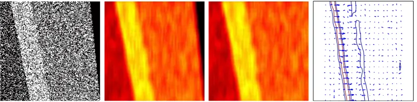
Figure 1: Four space-time representations of a simple synthetic version controlled document overV = {1,2}(see text for more details). The left panel displays the first component of (4) (non-smoothed array of unit vectors corresponding to words). The second and third panels display[γ(s, t)]1for the non-normalized and normalized representations respectively. The fourth panel displays the gradient vector field( ˙γs(s, t),γ˙t(s, t))(contour levels represent the gradient magnitude). The black portions of the first two panels correspond to zero padding due to unequal lengths of the different versions.
30, 40 and 120 words with the first segment in-creasing and the third segment dein-creasing at half the rate of the first segment with each revision. The length of the second segment was constant across the different versions. Figure 1 displays the nonsmoothed ragged array (4) (left), the non-normalized[γ(s, t)]1(middle left) and the
normal-ized[γ(s, t)]1(middle right).
While the left panel doesn’t distinguish much between the second and third segment the two smoothed representations display a nice seg-mentation of the space-time domain into three segments, each with roughly uniform values. The non-normalized representation (middle left) makes it easy to see that the total length of the version controlled document is increasing but it is not easy to judge what happens to the relative sizes of the three segments. The normalized rep-resentation (middle right) makes it easy to see that the first segment increases in size, the second is constant, and the third decreases in size. It is also possible to notice that the growth rate of the first segment is higher than the decay rate of the third.
3 Visualizing Change in Space-Time
We apply the space-time representation to four tasks. The first task, visualizing change, is de-scribed in this section. The remaining three tasks are described in the next three section.
The space-time domainΩrepresents the union of all document versions and all document posi-tions. Some parts of Ω are more homogeneous and some are less in terms of their local word dis-tribution. Locations in Ω where the local word distribution substantially diverges from its
neigh-bors correspond to sharp content transitions. On the other hand, locations whose word distribution is more or less constant correspond to slow con-tent variation.
We distinguish between three different types of changes. The first occurs when the word content changes substantially between neighboring doc-ument positions within a certain docdoc-ument ver-sion. As an example consider a document loca-tion whose content shifts from high level introduc-tory motivation to a detailed technical description. Such change is represented by
γ˙s(s, t)2 =
A second type of change occurs when a certain document position undergoes substantial change in local word distribution across neighboring ver-sions. An example is erroneous content in one version being heavily revised in the next version. Such change along the time axis corresponds to the magnitude of
Expression (6) may be used to measure the in-stantaneous rate of change in the local word dis-tribution. Alternatively, integrating (6) provides a global measure of change
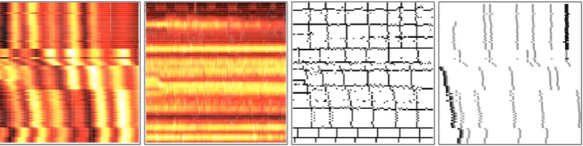
Figure 2: Gradient and edges for a portion of the version controlled Wikipedia Religion article. The left panel displays
γ˙s(s, t)2 (amount of change across document locations for different versions). The second panel displays
γ˙t(s, t)2
(amount of change across versions for different document positions). The third panel displays the local maxima of
γ˙s(s, t)2 +
γ˙t(s, t)2 which correspond to potential edges, either vertical lines (section and subsection boundaries) or horizontal lines (between substantial revisions). The fourth panel displays boundaries of sections and subsections as black and gray lines respectively.
the total amount of version change across differ-ent documdiffer-ent positions. h(s)may be used to de-tect document regions undergoing repeated sub-stantial content revisions andg(t)may be used to detect revisions in which substantial content has been modified across the entire document.
We conclude with the integrated directional derivative
1
0
˙
αs(r) ˙γs(α(r)) + ˙αt(r) ˙γt(α(r))2dr (8)
whereα : [0,1]→ Ωis a parameterized curve in the space-time and α˙ its tangent vector. Expres-sion (8) may be used to measure change along a dynamically moving document anchor such as the boundary between two book chapters. The space coordinate of such anchor shifts with the version number (due to the addition and removal of con-tent across versions) and so integrating the gra-dient across one of the two axis as in (7) is not appropriate. Definingα(r)to be a parameterized curve in space-time realizing the anchor positions
(s, t) ∈Ωacross multiple revisions, (8) measures the amount of change at the anchor point.
3.1 Experiments
The right panel of Figure 1 shows the gradient vector field corresponding to the synthetic ver-sion controlled document described in the previ-ous section. As expected, it tends to be orthog-onal to the segment boundaries. Its magnitude is displayed by the contour lines which show highest magnitudes around segment boundaries.
Figure 2 shows the norm γ˙s(s, t)2 (left), γ˙t(s, t)2 (middle left) and the local maxima
of γ˙s(s, t)2 +γ˙t(s, t)2 (middle right) for a
portion of the version controlled Wikipedia Re-ligion article. The first panel shows the amount of change in local word distribution within doc-uments. High values correspond to boundaries between sections, topics or other document seg-ments. The second panel shows the amount of change as one version is replaced with another. It shows which revisions change the word distri-butions substantially and which result in a rela-tively minor change. The third panel shows only the local maxima which correspond to edges be-tween topics or segments (vertical lines) or revi-sions (horizontal lines).
4 Edge Detection
In many cases documents may be divided to semantically coherent segments. Examples of text segments include individual news stories in streaming broadcast news transcription, sections in article or books, and individual messages in a discussion board or an email trail. For non-version controlled documents finding the text segments is equivalent to finding the boundaries or edges be-tween consecutive segments. See (Hearst, 1997; Beeferman et al., 1999; McCallum et al., 2000) for several recent studies in this area.
Things get a bit more complicated in the case of version controlled documents. Segments, and their boundaries exist in each version. As in case of image processing, we may view segment boundaries as edges in the space-time domain
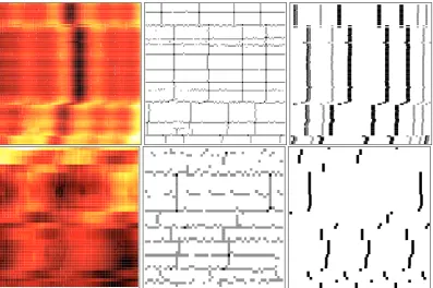
Figure 3: Gradient and edges of a portion of the version controlled Atlanta Wikipedia article (top row) and the Google Wave Amazon Kindle FAQ (bottom row). The left column displays the magnitude of the gradient in both space and time
γ˙s(s, t)2 +
γ˙t(s, t). The middle column displays the local maxima of the gradient magnitude (left column). The right column displays the actual segment boundaries as vertical lines (section headings for Wikipedia and author change in Google Wave). The gradient maxima corresponding to vertical lines in the middle column matches nicely the Wikipedia section boundaries. The gradient maxima corresponding to horizontal lines in the middle column correspond nicely to major revisions indicated by a discontinuities in the location of the section boundaries.
in a two dimensional geographical map.
Assuming all edges are correctly identified, we can easily identify the segments as the interior points of the closed boundaries. In general, how-ever, attempts to identify segment boundaries or edges will only be partially successful. As a result predicted edges in practice are not closed and do not lead to interior segments. We consider now the task of predicting segment boundaries or edges in
Ωand postpone the task of predicting a segmenta-tion to the next secsegmenta-tion.
Edges, or transitions between segments, corre-spond to abrupt changes in the local word dis-tribution. We thus characterize them as points in Ω having high gradient value. In particu-lar, we distinguish between vertical edges (transi-tions across document posi(transi-tions), horizontal edges (transitions across versions), and diagonal edges (transitions across both document position and version). These three types of edges may be di-agnosed based on the magnitudes of γ˙s, γ˙t, and
˙
α1γs+ ˙α2γtrespectively.
4.1 Experiments
Besides the synthetic data results in Figure 2, we conducted edge detection experiments on six different real world datasets. Five datasets are Wikipedia.com articles: Atlanta, Religion, Lan-guage, European Union, and Beijing. Religion and European Union are version controlled docu-ments with relatively frequent updates, while At-lanta, language, and Beijing have less frequent changes. The sixth dataset is the Google Wave Amazon Kindle FAQ which is a less structured version controlled document.
Preprocessing included removing html tags and pictures, word stemming, stop-word removal, and removing any non alphabetic characters (numbers and punctuations). The section heading informa-tion of Wikipedia and the informainforma-tion of author of each posting in Google Wave is used as ground truth for segment boundaries. This information was separated from the dataset and was used for training and evaluation (on testing set).
Article Rev. Voc. ppp(((yyy))) Error Rate F1 Measure
Size a b c a b c
Atlanta 2000 3078 0.401 0.401 0.424 0.339 0.000 0.467 0.504
Religion 2000 2880 0.403 0.404 0.432 0.357 0.000 0.470 0.552 Language 2000 3727 0.292 0.292 0.450 0.298 0.000 0.379 0.091 European Union 2000 2382 0.534 0.467 0.544 0.435 0.696 0.397 0.663
Beijing 2000 3857 0.543 0.456 0.474 0.391 0.704 0.512 0.682
Amazon Kindle FAQ 100 573 0.339 0.338 0.522 0.313 0.000 0.436 0.558
Figure 4: Test set error rate and F1 measure for edge prediction (section boundaries in Wikipedia articles and author change in Google Wave). The space-time domainΩwas divided to a grid with each cell labeled edge (y = 1) or no edge (y= 0) depending on whether it contained any edges. Method a corresponds to a predictor that always selects the majority class. Method b corresponds to the TextTiling test segmentation algorithm (Hearst, 1997) without paragraph boundaries information. Method c corresponds to a logistic regression classifier whose feature set is composed of statistical summaries (mean, median, max, min) ofγ˙s(s, t)within the grid cell in question as well as neighboring cells.
the version controlled Wikipedia articles Religion and Atlanta. The local gradient maxima nicely match the segment boundaries which lead us to consider training a logistic regression classifier on a feature set composed of gradient value statis-tics (min, max, mean, median ofγ˙s(s, t)in the
appropriate location as well as its neighbors (the space-time domainΩwas divided into a finite grid where each cell either contained an edge (y = 1) or did not (y= 0)). The table in Figure 4 displays the test set accuracy and F1 measure of three pre-dictors: our logistic regression (method c) as well as two baselines: predicting edge/no-edge based on the marginal p(y)distribution (method a) and TextTiling (method b) (Hearst, 1997) which is a popular text segmentation algorithm. Since we do not assume paragraph information in our experi-ment we ignored this component and considered the document as a sequence with w = 20 and 29 minimum depth gaps parameters (see (Hearst, 1997)). We conclude from the figure that the gra-dient information leads to better prediction than TextTiling (on both accuracy and F1 measure).
5 Segmentation
As mentioned in the previous section, predicting edges may not result in closed boundaries. It is possible to analyze the location and direction of the predicted edges and aggregate them into a se-quence of closed boundaries surrounding the seg-ments. We take a different approach and partition points inΩtokdistinct values or segments based on local word content and space-time proximity.
For two points(s1, t2),(s2, t2)∈Ωto be in the
same segment we expectγ(s1, t1)to be similar to
γ(s2, t2) and for (s1, t1) to be close to (s2, t2).
The first condition asserts that the two locations discuss the same topic. The second condition as-serts that the two locations are not too far from each other in the space time domain. More specif-ically, we propose to segmentΩby clustering its points based on the following geometry
d((s1, t1),(s2, t2)) =dH(γ(s1, t1), γ(s2, t2)) +c1(s1−s2)2+c2(t1−t2)2 (9)
wheredH :PV ×PV →Ris Hellinger distance
d2H(u, v) = V
i=1
(√ui−√vi)2. (10)
The weightsc1, c2 are used to balance the
contri-butions of word content similarity with the simi-larity in time and space.
5.1 Experiments
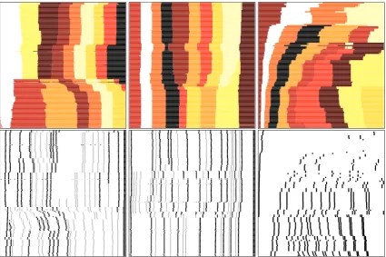
Figure 5 displays the ground truth segment bound-aries and the segmentation results obtained by ap-plyingk-means clustering (k= 11) to the metric (9). The figure shows that the predicted segments largely match actual edges in the documents even though no edge or gradient information was used in the segmentation process.
6 Predicting Future Operations
The fourth and final task is predicting a future revision dl+1 based on the smoothed
Figure 5:Predicted segmentation (top) and ground truth segment boundaries (bottom) of portions of the version controlled Wikipedia articles Religion (left), Atlanta (middle) and the Google Wave Amazon Kindle FAQ(right). The predicted segments match the ground truth segment boundaries. Note that the first 100 revisions are used in Google Wave result. The proportion of the segments that appeared in the beginning is keep decreasing while the revisions increases and new segments appears.
terms ofΩ, this means predicting features associ-ated withγ(s, t), t≥tbased onγ(s, t), t < t.
6.1 Experiments
We concentrate on predicting whether Wikipedia edits are reversed in the next revision. This ac-tion, marked by a label UNDO or REVERT in the Wikipedia API, is important for preventing con-tent abuse or removing immature concon-tent (by pre-dicting ahead of time suspicious revisions).
We predict whether a version will undergo UNDO in the next version using a support vec-tor machine based on statistical summaries (mean, median, min, max) of the following feature set γ˙s(s, t), ¨γs(s, t), γ˙t(s, t)), γ˙t(s, t),
g(h), and h(s). Figure 6 shows the test set er-ror and F1 measure for the logistic regression based on the smoothed space-time representation (method c), as well as two baselines. The first baseline (method a) predicts the majority class and the second baseline (method b) is a logistic regression based on the term frequency content of the current test version. Using the derivatives of γ, we obtain a prediction that is better than
choos-ing majority class or logistic regression based on word content. We thus conclude that the deriva-tives above provide more useful information (re-sulting in lower error and higher F1) for predicting future operations than word content features.
7 Related Work
While document analysis is a very active research area, there has been relatively little work on ex-amining version controlled documents. Our ap-proach is the first to consider version controlled documents as continuous mappings from a space-time domain to the space of local word distribu-tions. It extends the ideas in (Lebanon et al., 2007) of using kernel smoothing to create a continuous representation of documents. In fact, our frame-work generalizes (Lebanon et al., 2007) as it re-verts to it in the case of a single revision.
Article Rev. Voc. ppp(((yyy))) Error Rate F1 Measure
Size a b c a b c
Atlanta 2000 3078 0.218 0.219 0.313 0.212 0.000 0.320 0.477 Religion 2000 2880 0.123 0.122 0.223 0.125 0.000 0.294 0.281 Language 2000 3727 0.189 0.189 0.259 0.187 0.000 0.334 0.455 European Union 2000 2382 0.213 0.208 0.331 0.209 0.000 0.275 0.410 Beijing 2000 3857 0.137 0.137 0.219 0.136 0.000 0.247 0.284
Figure 6: Error rate and F1 measure over held out test set of predicting future UNDO operation in Wikipedia articles. Method a corresponds to a predictor that always selects the majority class. Method b corresponds to a logistic regression based on the term frequency vector of the current version. Method c corresponds a logistic regression that uses summaries (mean, median, max, min) ofγ˙s(s, t),γ˙s(s, t),g(t), andh(s).
1997; Beeferman et al., 1999; McCallum et al., 2000) with (Hearst, 1997) being the closest in spirit to our approach. An influential model for topic modeling within and across documents is la-tent Dirichlet allocation (Blei et al., 2003; Blei and Lafferty, 2006). Our approach differs in be-ing fully non-parametric and in that it does not require iterative parametric estimation or integra-tion. The interpretation of local word smoothing as a non-parametric statistical estimator (Lebanon et al., 2007) may be extended to our paper in a straightforward manner.
Several attempts have been made to visualize themes and topics in documents, either by keep-ing track of the word distribution or by dimen-sionality reduction techniques e.g., (Fortuna et al., 2005; Havre et al., 2002; Spoerri, 1993; Thomas and Cook, 2005). Such studies tend to visualize a corpus of unrelated documents as opposed to or-dered collections of revisions which we explore.
8 Summary and Discussion
The task of analyzing and visualizing version con-trolled document is an important one. It allows external control and monitoring of collaboratively authored resources such as Wikipedia, Google Wave, and CVS or SVN documents. Our frame-work is the first to develop analysis and visualiza-tion tools in this setting. It presents a new rep-resentation for version controlled documents that uses local smoothing to map a space-time domain
Ω to the simplex of tf vectors PV. We
demon-strate the applicability of the representation for four tasks: visualizing change, predicting edges, segmentation, and predicting future revision oper-ations.
Visualizing changes may highlight significant structural changes for the benefit of users and help the collaborative authoring process. Improved edge prediction and text segmentation may assist in discovering structural or semantic changes and their evolution with the authoring process. Pre-dicting future operation may assist authors as well as prevent abuse in coauthoring projects such as Wikipedia.
The experiments described in this paper were conducted on synthetic, Wikipedia and Google Wave articles. They show that the proposed for-malism achieves good performance both qualita-tively and quantitaqualita-tively as compared to standard baseline algorithms.
It is intriguing to consider the similarity be-tween our representation and image processing. Predicting segment boundaries are similar to edge detection in images. Segmenting version con-trolled documents may be reduced to image seg-mentation. Predicting future operations is similar to completing image parts based on the remain-ing pixels and a statistical model. Due to its long and successful history, image processing is a good candidate for providing useful tools for version controlled document analysis. Our framework fa-cilitates this analogy and we believe is likely to re-sult in novel models and analysis tools inspired by current image processing paradigms. A few po-tential examples are wavelet filtering, image com-pression, and statistical models such as Markov random fields.
Acknowledgements
References
Beeferman, D., A. Berger, and J. D. Lafferty. 1999. Statistical models for text segmentation. Machine
Learning, 34(1-3):177–210.
Blei, D. and J. Lafferty. 2006. Dynamic topic models. In Proc. of the International Conference on Machine
Learning.
Blei, D., A. Ng, , and M. Jordan. 2003. Latent dirich-let allocation. Journal of Machine Learning Re-search, 3:993–1022.
Fortuna, B., M. Grobelnik, and D. Mladenic. 2005. Visualization of text document corpus. Informatica, 29:497–502.
Havre, S., E. Hetzler, P. Whitney, and L. Nowell. 2002. Themeriver: Visualizing thematic changes in large document collections. IEEE Transactions on
Visu-alization and Computer Graphics, 8(1).
Hearst, M. A. 1997. Texttiling: Segmenting text into multi-paragraph subtopic passages. Computational
Linguistics, 23(1):33–64.
Lebanon, G., Y. Mao, and J. Dillon. 2007. The lo-cally weighted bag of words framework for doc-uments. Journal of Machine Learning Research,
8:2405–2441, October.
McCallum, A., D. Freitag, and F. Pereira. 2000. Max-imum entropy Markov models for information ex-traction and segmentation. In Proc. of the
Interna-tional Conference on Machine Learning.
Spoerri, A. 1993. InfoCrystal: A visual tool for infor-mation retrieval. In Proc. of IEEE Visualization.
Thomas, J. J. and K. A. Cook, editors. 2005.
Illu-minating the Path: The Research and Development Agenda for Visual Analytics. IEEE Computer
Soci-ety.
Wand, M. P. and M. C. Jones. 1995. Kernel
Smooth-ing. Chapman and Hall/CRC.
Wang, C., D. Blei, and D. Heckerman. 2009. Continu-ous time dynamic topic models. In Proc. of