ECE-320 Lab 7: Discrete-Time PID and PI Controllers and sisotool
Overview
In this lab you will be controlling both of the one degree of freedom systems you previously modeled using discrete-time PID and PI controllers. Both one degree of freedom systems must be controlled, and if there are two people in your lab group each lab partner should do a different system.
You will need to download the files for Lab 7 from the class website.
Design Specifications: For each of your systems, you should try and adjust your parameters until you have achieved the following:
Rectilinear Systems (Model 210)
Settling time less than 1.5 seconds.
Steady state error less than 0.1 cm for a 1 cm step, and less than 0.05 cm for a 0.5 cm step
Percent Overshoot less than 25%
Your memo should include four graphs for each of the 1 dof systems you used (a PID controller and a PI controller for each system, two different sampling intervals Your memo should compare the
difference between the predicted response (from the model) and the real response (from the real system) for each of the systems.
Background/Review
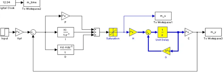
The file DT_PID.mdl is a Simulink model that implements a discrete-time PID controller. It is somewhat unusual in that the plant is represented in state-variable form, but this is the usual form we will using in this class. The Simulink model looks like the model shown in Figure 1:
The file DT_PID_driver.m is the Matlab file that runs this code. We will be utilizing Matlab’s sisotool for determining the pole placement and the values of the gains.
Before we go on, we need to remember the following two things about discrete-time systems:
For stability, all poles of the system must be within the unit circle. However, zeros can be outside of the unit circle.
The closer to the origin your dominant poles are, the faster your system will respond. However, the control effort will generally be larger.
The basic transfer function form of the components of a discrete-time PID controller are as follows:
Proportional (P) term :
Integral (I) term:
Derivative (D) term :
PI Controller: To construct a PI controller, we add the P and I controllers together to get the overall transfer function:
In sisotool this will be represented as
In order to get the coefficients we need out of the sisotool format we equate coefficients to get:
PID Controller: To construct a PID controller, we add the P, I, and D controllers together to get the overall transfer function:
In sisotool this will be represented as
For the PID controller, we can have either two complex conjugate zeros or two real zeros.
Sisotool (Brief) Example
Run the Matlab program DT_PID_driver.m. This program is set up to read the data file
bobs_210_model.mat, which is a continuous time state variable model for a one degree of freedom rectilinear system, construct an equivalent discrete-time system using a sample and hold with a delay (the sample time is given by Ts), and implement a P controller with gain 0.0116. It will put the value of
the transfer function for your system, , in your workspace. Now we are ready for sisotool.
Getting Started
Type sisotool in the command window
Click close when the help window comes up
Click on View, then Design Plots Configuration, and turn off all plots except the Root Locus plot (set the Plot Type to Root Locus for Plot 1, and set the Plot Type to None for all other Plots)
Loading the Transfer Function
In the SISO Design window, Click on file → import.
We will usually be assigning Gp(z) to block G (the plant). Under the System heading, click on the line that indicates G, then click on Browse.
Choose the available Model that you want assigned to G (Click on the appropriate line) and then click on Import, and then on Close.
Click OK on the System Data (Import Model) window
Once the transfer function has been entered, the root locus is displayed. Make sure the poles and zeros of your plant are where you think they should be. Note that there will be three poles (one at zero) for our second order system since for this system there is a delay inserted by the Simulink model.
Generating the Step Response
Click on Analysis → Response to Step Command (the system is unstable at this point)
You will probably have two curves on your step response plot. To just get the output, type Analysis → Other Loop Responses. If you only want the output, then only r to y is checked, and then click OK. However, sometimes you will also want the r to u output, since it shows the control effort for P, I, and PI controllers.
You can move the location of the pole in the root locus plot by putting the cursor over the pink button and holding the left mouse button down as you move the pole locations. You should note that the step response changes as the pole locations change.
Entering a Compensator (controller): We will implement a PI controller here
Click on Designs, then Edit Compensators.
Right click in the Dynamics window to enter real poles and zeros. You will be able to changes these values very easily later. Since we want a PI controller, we need a pole to be a 1 and we need to be able to change the value of the zero. For now assume the zero is at -1.
Look at the form of C to be sure it's what you intended, and then look at the root locus with the compensator.
You can again see how the step response changes with the compensator by moving the locations of the zero (grab the pink dot and slide it) and moving the gain of the system (grab the squares and drag them). Remember we need all poles and zeros to be inside the unit circle for stability!
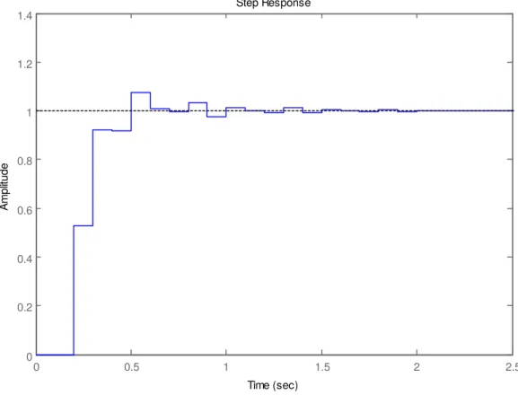
Move the pole and zero around until the zero is approximately -0.295 and the gain is approximately 0.0563. You should get a figure like that shown in Figure 2.
Step Response
Time (sec)
Am
pl
itu
de
0 0.5 1 1.5 2 2.5
0 0.2 0.4 0.6 0.8 1 1.2 1.4
Figure 2. Discrete-time example with w PI controller.
Adding Constraints
Right Click on the Root Locus plot, and choose Design Requirements then either New to add new constraints, or Edit to edit existing constraints.
At this point you have a choice of various types of constraints.
Printing/Saving the Figures:
To save a figure sisotool has created, click File → Print to Figure
Odds and Ends :
You may want to fix the axes. To do this,
Right click on the Root Locus Plot
Choose Properties
Choose Limits
Set the limits and turn the Auto Scale off
You may also want to put on a grid, as another method of checking your answers. To do this, right click on the Root Locus plot, then choose Grid
It is easiest if you use the zero/pole/gain format for the compensators. To do this click on Edit → SISO Tool Preferences → Options and click on zero/pole/gain.
Back to Matlab.
Determine the correct values of a and K
Enter these in the Matlab code DT_PID_driver.m
Modify DT_PID_driver.m to compute the proportional and integral gains
For each of your two 1 dof systems, you will need to go through the following steps:
Step 1: Set up the 1 dof system exactly the way it was when you determined its model parameters.
Step 2: Modify DT_PID_driver.m to read in the correct model file. You may have to copy this model file to the current folder.
Step 3: Modify DT_PID_driver.m to use the correct saturation_level for the system you are using.
Step 4: Set the sampling interval to 0.1 seconds (the first time) and then 0.05 seconds (the second time).
Step 5: PID and PI Control
Design a PID and then a PI controller using sisotool to meet the design specs. Use a constant prefilter (i.e., a number, most likely the number 1)
Implement the correct gains into DT_PID_driver.m
Simulate the system for 2.0 seconds. If the design constrains are not met, or the control effort hits a limit, redesign your controller (you might also try a lower input signal). Try and stay away from the maximum allowed control values as much as possible, they are not as good a predictor with discrete-time systems as with continuous time systems.
Reset the system using ECPDSPReset.mdl
Compile the correct closed loop ECP Simulink driver (Model210_DT_PID.mdl), connect to the system, and run the simulation.