Nonlinear and Hybrid Systems Verification
Thesis by
Stephen Prajna
In Partial Fulfillment of the Requirements for the Degree of
Doctor of Philosophy
California Institute of Technology Pasadena, California
2005
c
Acknowledgements
I would like to express my gratitude to my advisor, Professor John Doyle, for ad-mitting me to Caltech and for providing his guidance and advice during my years at Caltech. Working with John has opened a whole new world to me. I really appreciate the intellectual freedom and the “think outside the box” spirit that he has given to me and his other students.
My acknowledgements also go to Professors Anders Rantzer, Pablo Parrilo, Ali Jadbabaie, and George Pappas for being my mentors. It has been an honor for me to work with them. In addition, I thank them for inviting me to visit Lund, ETH, and Penn at various times during my studies. Back at Caltech, thanks to Professors Richard Murray, Jerrold Marsden, Mani Chandy, and Hideo Mabuchi for serving on my committees and providing constructive feedbacks on my work.
I would like to thank Professors Manfred Morari, Arjan van der Schaft, Torkel Glad, Karl Henrik Johansson, Bjarne Foss, and Raffaello d’Andrea for their hospital-ity when I visited their institutions in the spring and summer of 2004. I also thank Professor Yaser Abu-Mostafa for supporting one of my conference trips in the same year.
To my friends Antonis Papachristodoulou, Domitilla del Vecchio, Xin Liu, Harish Bhat, Melvin Flores, Melvin Leok, and Shreesh Mysore, and the rest of CDS, thank you for the camaraderie and the good time that we had.
Abstract
Complex behaviors that can be exhibited by hybrid systems make the verification of such systems both important and challenging. Due to the infinite number of possi-bilities taken by the continuous state and the uncertainties in the system, exhaustive simulation is impossible, and also computing the set of reachable states is generally intractable. Nevertheless, the ever-increasing presence of hybrid systems in safety critical applications makes it evident that verification is an issue that has to be ad-dressed.
In this thesis, we develop a unified methodology for verifying temporal properties of continuous and hybrid systems. Our framework does not require explicit compu-tation of reachable states. Instead, functions of state termed barrier certificates and density functions are used in conjunction with deductive inference to prove properties such as safety, reachability, eventuality, and their combinations. As a consequence, the proposed methods are directly applicable to systems with nonlinearity, uncertainty, and constraints. Moreover, it is possible to treat safety verification of stochastic sys-tems in a similar fashion, by computing an upper-bound on the probability of reaching the unsafe states.
Contents
Acknowledgements iii
Abstract iv
1 Introduction 1
1.1 Background . . . 1
1.2 Contributions and Outline . . . 4
1.3 Notations . . . 5
2 Worst-Case Safety Verification 7 2.1 Continuous Systems . . . 9
2.1.1 Convex Conditions . . . 9
2.1.2 Non-Convex Conditions . . . 12
2.1.3 Incorporating Constraints . . . 13
2.2 Hybrid Systems . . . 16
2.2.1 Modelling Framework . . . 16
2.2.2 Conditions for Safety . . . 18
2.2.3 Hybrid Systems with Constraints . . . 21
2.3 Computational Method . . . 22
2.3.1 Sum of Squares Optimization . . . 23
2.3.2 Direct Computation . . . 25
2.3.3 Iterative Computation . . . 29
2.4 Examples . . . 31
2.4.2 Hybrid System . . . 33
2.4.3 Limit of Design . . . 34
2.5 Appendix: Non-Convex Conditions . . . 36
3 Stochastic Safety Verification 39 3.1 Continuous Systems . . . 41
3.2 Hybrid Systems . . . 46
3.2.1 Piecewise Deterministic Markov Processes . . . 46
3.2.2 Switching Diffusion Processes . . . 49
3.2.3 Stochastic Hybrid Systems . . . 51
3.3 Examples . . . 54
3.3.1 Stochastic Differential Equation . . . 54
3.3.2 Switching Diffusion Process . . . 55
4 Reachability and Eventuality Verification 58 4.1 Discrete Example . . . 60
4.2 Continuous Systems . . . 64
4.2.1 Safety and Reachability Verification . . . 64
4.2.2 Eventuality Verification . . . 70
4.2.3 Other Verification . . . 72
4.3 Hybrid Systems . . . 74
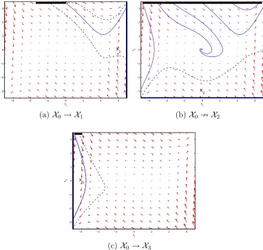
4.4 Examples . . . 75
4.4.1 Successive Safety and Reachability Refinements . . . 75
4.4.2 Eventuality and Eventuality – Safety Verification . . . 76
5 On the Necessity of Barrier Certificates 81 5.1 A Converse Theorem . . . 81
5.2 Some Remarks . . . 87
6 Conclusions 91
List of Figures
2.1 Phase portrait of the system in Section 2.4.1. . . 32
2.2 Discrete transition diagram of the system in Section 2.4.2. . . 33
2.3 Block diagram of the system in Section 2.4.3. . . 35
3.1 Phase portrait of the system in Section 3.3.1. . . 55
3.2 Phase portrait of the system in Section 3.3.2. . . 57
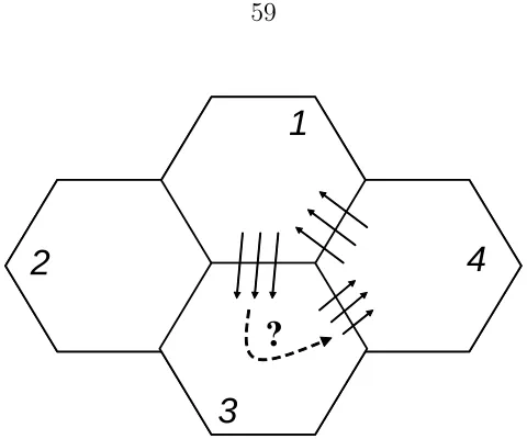
4.1 System analysis by abstraction. . . 59
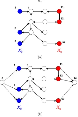
4.2 Verification of a simple discrete transition system. . . 61
4.3 Proving the reachability of X1 and X3 fromX0 in Section 4.4.1. . . 77
4.4 Possible transitions from X0 toX1, X2, and X3 in Section 4.4.1. . . 78
List of Tables
Chapter 1
Introduction
1.1
Background
Much research effort has been devoted to the development of hybrid systems theory in the recent years. Hybrid systems [48,92] are systems whose dynamics involve both continuous and discrete processes in interactions. Research on hybrid systems (see, e.g., [5, 7, 8, 25, 45, 51, 52, 89]) is partly motivated by the ubiquity of engineering and physical systems that are best modelled as such systems. One important example is the class of embedded and software-based control systems, which consist of discrete controllers, typically logical and event-based, interconnected with analog and often nonlinear actuators, sensors, and plants. Embedded and software-based systems have become increasingly ubiquitous in our everyday life. In fact, the trend shows that next generation control systems will be mostly of this type [53, 56].
when correctness, robustness, and optimality are of paramount importance, which renders design by informal reasoning combined with trial and error ineffective.
Besides the more traditional properties such as stability and input-output per-formance, properties of interest in hybrid systems also include safety, reachability, and eventuality. In principle, safety verification aims to show that starting from any initial condition in some prescribed set, a system cannot evolve to some unsafe region in the state space. On the other hand, reachability verification aims to show that for
some — and eventuality verification for all — initial conditions in some prescribed set, the system will evolve to some target region in the state space. The above prop-erties are the most relevant when the system specifications are given in temporal logic formulas [36, 46] such as
(from a multi-vehicle coordination scenario): “if Agent 1 starts at zoneA
and Agent 2 starts at zone B, then under the given control strategy, • Agent 1 will reach zoneC in finite time,
• Agent 2 will not reach zone Dbefore Agent 1 reaches C,
• both Agent 1 and Agent 2 will never enter a forbidden zoneE at any time,”
which is the kind of specifications that seem likely to dominate next generation control systems. These verification questions are by no mean easy to answer, as for very simple classes of hybrid systems they are known to be undecidable already [30].
the use of an efficient data structure called ordered binary decision diagrams [18] has allowed model checking of systems with an astronomical number of states. Still, when the number of possible states is infinite, such as when the state space is continuous, model checking is no longer applicable. Indeed, the difficulty of applying model checking to hybrid systems is caused by the continuous part of their state space. Deductive verification, on the other hand, verifies system properties through formal deduction based on a set of inference rules. Deductive verification is applicable to infinite state systems, but has a drawback in the sense that guidance from a user is almost always needed in the process.
From control theory, there exist also comprehensive bodies of techniques for veri-fying properties of continuous systems such as stability, performance, robust stability, robust performance, and so on (see e.g., [40, 98]). These techniques are deductive in nature, since the systems considered have an infinite number of states. If the systems have a special structure (e.g., linear), then the verification can be automated. Unfor-tunately, the techniques are geared to verify properties that are expressed in terms of Lyapunov stability or signal/system norms, and as such are not directly applicable to verification of properties such as safety, reachability, and eventuality, let alone more general temporal logic formulas.
1.2
Contributions and Outline
The objective of this thesis is to develop unified theoretical and computational frame-works that will facilitate automated verification of properties such as safety, reach-ability, and eventuality for continuous and hybrid systems. In doing so, we have used theoretical concepts calledbarrier certificates and density functions, in addition to a computational relaxation framework called sum of squares optimization, which involves sum of squares decompositions of multivariate polynomials, semidefinite pro-gramming, and real algebraic geometry. The contributions and outline of the thesis are as follows.
In Chapter 2, we introduce the concept of barrier certificates and propose us-ing them for safety verification of continuous and hybrid systems in the worst-case setting. A barrier certificate is a function (or a set of functions) of state satisfying some inequalities on both the function itself and its derivative along the flow of the system. In this setting, a barrier certificate proves that all possible system trajec-tories starting from a given initial set cannot reach a given unsafe region. The use of barrier certificates for verifying safety is analogous to the use of Lyapunov func-tions for proving stability, and eliminates the need to propagate sets of states. As a consequence, our approach is directly applicable to systems with nonlinearity, un-certainty, constraints, and hybrid dynamics. We also propose using a class of convex relaxation, i.e., sum of squares optimization, to compute barrier certificates for sys-tems whose descriptions are in terms of polynomials. Sum of squares optimization provides a hierarchical way to search for barrier certificates, where at each level the computational cost grows polynomially with respect to the system size. Because of this, our methodology seems to be more scalable than many other existing methods that can handle nonlinear continuous and hybrid systems. This chapter is based on the papers [65, 66].
system is not safe. Indeed, it is more natural to consider safety verification with probabilistic interpretation, e.g., to prove that the probability of reaching the unsafe set is lower than some safety margin. This is the subject of Chapter 3. Our method uses supermartingales as barrier certificates and upper-bounds the reach probability using a certain supermartingale inequality. The method is applicable to a large class of stochastic continuous and hybrid systems with polynomial descriptions, and is the first proposed computational method that can provide a verifiable upper bound on the reach probability. This chapter is based on the paper [67].
In Chapter 4, we consider the duality relation between proving safety and reach-ability. Using insights from the linear programming duality appearing in the discrete shortest path problem and the concept of density functions, we show that proving reachability or eventuality in continuous systems can also be performed by solving a convex optimization problem. Convex programs involving barrier certificates and density functions for verifying safety, reachability, eventuality, and some other tem-poral specifications are formulated. The chapter is based on the paper [76].
In Chapter 5, the duality relation between safety and reachability is used to prove a converse theorem for safety verification using barrier certificates. Under reasonable technical conditions, we prove that there exists a barrier certificate for a nonlinear continuous system if and only if the safety property holds. The chapter is based on the paper [75].
We end the thesis in Chapter 6 by presenting some conclusions and suggestions for future research.
1.3
Notations
We denote the set of real numbers by Rand the Euclideann-space byRn. The trace of ann×n matrixM, i.e., the sum of its diagonal elements, is denoted by Tr(M). In addition, we use int(X), cl(X), and ∂X to denote the interior, the closure, and the boundary of a set X ⊆Rn.
By f : X →Y we mean a function f mapping X ⊆ Rn to Y ⊆
the spaces of k-times continuously differentiable functions mapping X ⊆ Rn to Rm
by Ck(X,Rm), and when m = 1, we will write Ck(X). Correspondingly, the spaces of continuous functions on X are denoted by C(X,Rm) and C(X), equipped with the supremum norm if necessary. The zero subscript as in C1
0(Rn) indicates that the
functions have compact supports. The dual space of a normed linear space K, i.e., the space of all continuous linear functionals on K, is denoted by K∗. By hk∗, ki we
mean the value of a continuous linear functional k∗ ∈ K∗ applied to k∈ K.
For a differentiable function F :Rn →R, we define
∂F ∂x(x),
∂F ∂x1
(x) · · · ∂F
∂xn (x)
,
and
∂2F
∂x2(x),
∂2F
∂x2 1
(x) · · · ∂
2F
∂x1∂xn (x) ... . .. ...
∂2F
∂x1∂xn
(x) · · · ∂
2F
∂x2
n (x)
.
The divergence of a differentiable vector field f :Rn→
Rn,
∂f1
∂x1
(x) +...+ ∂fn
∂xn (x),
is denoted by ∇ ·f(x). The flow of ˙x=f(x) starting at x0 is denoted byφt(x0). For
a set Z ⊆Rn, we define φt(Z),{φt(x0) :x0 ∈Z}.
Chapter 2
Worst-Case Safety Verification
In this chapter, we consider safety verification of nonlinear continuous and hybrid systems in the worst-case setting. Some disturbance signal and model uncertainty may also be included in the system description. We want to verify that under any circumstances, there is no trajectory of the system that starts from a given set of possible initial states and goes to an unsafe region in the state space. Such anal-ysis is particularly important for safety critical systems like air traffic control [90], autonomous vehicle systems [33], and life support systems [28].
con-structing abstractions (i.e., discrete quotients) of the systems, and then performing model checking on the resulting discrete systems. See for instance [2,4,10,13,22,87,91]. We will present a method for safety verification that is different from the above approaches as it does not require computation of reachable sets, but instead relies on what we term barrier certificates. For a continuous system, a barrier certificate is a function of state satisfying a set of inequalities on both the function itself and its Lie derivative along the flow of the system. In the state space, the zero level set of a barrier certificate separates an unsafe region from all system trajectories starting from a set of possible initial states. Therefore, the existence of such a function provides an exact certificate/proof of system safety.
Similar to the Lyapunov approach for proving stability, the main idea here is to study properties of the system without the need to compute the flow explicitly. Although an over-approximation of the reachable set may also be used as a proof for safety, a barrier certificate can be much easier to compute when the system is nonlinear and uncertain. Moreover, barrier certificates can be easily used to verify safety in infinite time horizon. Note also that there are some connections between our method and viability theory [11], invariant set theory [11,14], and also the verification approaches in [37, 83, 88]. We will discuss these connections later as we progress.
Our method can be easily extended to handle hybrid systems. In the hybrid case, a barrier certificate is constructed from a set of functions of continuous state indexed by the system location1. Instead of satisfying the aforementioned inequalities in the
whole continuous state space, each function needs to satisfy the inequalities only within the invariant of the location. Functions corresponding to different locations are linked via appropriate conditions that must be satisfied during discrete transi-tions between the locatransi-tions. The idea is analogous to using multiple Lyapunov-like functions [38] for stability analysis of hybrid systems.
With this methodology, it is possible to treat a large class of hybrid systems, including those with nonlinear continuous dynamics, uncertainty, and constraints. When the vector fields of the system are polynomials and the sets in the system
de-1
scription are semialgebraic (i.e., described by polynomial equalities and inequalities), a tractable computational method called sum of squares optimization [61, 62, 69, 72] can be utilized for constructing a polynomial barrier certificate, e.g., using the soft-ware SOSTOOLS [69,72]. While the computational cost of this construction depends on the degrees of the vector fields and the barrier certificate in addition to the number of discrete locations and the continuous state dimension, for fixed polynomial degrees the complexity grows polynomially with respect to the other quantities. Hence, we expect our method to be more scalable than many other existing methods. Successful application of our method to a NASA life support system, which is a nonlinear hybrid system with six discrete modes and ten continuous state variables, has been reported in [28].
This chapter is organized as follows. In Section 2.1, safety verification of contin-uous systems is addressed. We present some conditions for barrier certificates which guarantee the safety of the system. Later in the same section, we incorporate con-straints into the framework. Safety verification of hybrid systems is then addressed in Section 2.2. Section 2.3 is devoted to computation of barrier certificates. Finally, Section 2.4 contains some examples illustrating the use of the methodology.
2.1
Continuous Systems
2.1.1
Convex Conditions
In this section, we address safety verification of continuous systems, to establish a foundation for the subsequent results. Consider a continuous system described by a set of ordinary differential equations in the state space form:
˙
x(t) = f(x(t), d(t)), (2.1)
the vector fieldf(x, d). At the least it will be continuous, which makesx(t) piecewise continuously differentiable.
In safety verification, only parts of trajectories that are contained in a given set X ⊆Rn and that start from a given set of possible initial states X0 ⊆ X are
consid-ered. We denote the unsafe region of the system by Xu, with Xu ⊆ X. With these notations, the safety property in the worst-case setting can be defined as follows. The definition can be directly extended for other classes of systems as needed.
Definition 2.1 (Safety) Given the system (2.1), the state set X ⊆ Rn, the initial set X0 ⊆ X, the unsafe set Xu ⊆ X, and the disturbance set D ⊆ Rm, we say
that the safety property holds if there exist no time instant T ≥ 0 and a piecewise continuous and bounded disturbanced: [0, T]→ D that gives rise to an unsafe system trajectory, i.e., a trajectory x : [0, T] → Rn satisfying x(0) ∈ X0, x(T) ∈ Xu, and
x(t)∈ X ∀t∈[0, T].
Our method for verifying safety relies on the existence of what we will call barrier certificate. For continuous systems, the following proposition states the conditions that are satisfied by a barrier certificate.
Proposition 2.2 Let the system x˙ = f(x, d) and the sets X ⊆ Rn, X0 ⊆ X, Xu ⊆
X, D ⊆ Rm be given, with f ∈ C(Rn+m,Rn). Suppose there exists a differentiable function B :Rn →R such that
B(x)≤0 ∀x∈ X0, (2.2)
B(x)>0 ∀x∈ Xu, (2.3)
∂B
∂x(x)f(x, d)≤0 ∀(x, d)∈ X × D, (2.4)
then the safety of the system in the sense of Definition 2.1 is guaranteed.
Proof. Our proof is by contradiction. Assume that there exists a barrier certificate
an initial condition x0 ∈ X0 such that a trajectory x(t) of the system starting at
x(0) = x0 satisfies x(t) ∈ X for all t ∈ [0, T] and x(T) ∈ Xu. Condition (2.4)
implies that the derivative ofB(x(t)) with respect to time is non-positive on the time interval [0, T]. A direct consequence of this (which for example can be shown using the mean value theorem) is thatB(x(T)) must be less than or equal toB(x(0)), which is contradictory to (2.2)–(2.3). Thus the initial hypothesis is not correct: the system must be safe.
A function B(x) satisfying the conditions in Proposition 2.2 is termed a barrier certificate. The zero level set of a barrier certificate “provides a barrier” between possible system trajectories and the given unsafe region, in the sense that no trajectory of the system starting from the initial set can cross this level set to reach the unsafe region (cf. Section 2.4.1 for a visual illustration). In proving that the system is safe, no explicit computation of system trajectories nor reachable sets is required.
In the above proposition, we have assumed that the unknown disturbance input can vary arbitrarily fast. If the variation of the disturbance is bounded (for example, when there are uncertain parameters, which can be regarded as time-invariant distur-bance), then a less conservative verification can be performed by considering a barrier certificate B(x, d) that also depends on the instantaneous value of the disturbance and modifying (2.2)–(2.4) accordingly. For example, in (2.4) we need to take into account the extra derivative term ∂B∂d(x, d) ˙d, with the disturbance variation ˙d taking its value in some bounded set.
Note that the set of barrier certificates satisfying the conditions in Proposition 2.2 is convex. This can be established by taking arbitraryB1(x) andB2(x) satisfying the
above conditions and showing that for all α ∈[0,1], B(x) =αB1(x) + (1−α)B2(x)
satisfies the conditions as well. The convexity property is very beneficial for the computation of B(x). As we will see later in Section 2.3, a barrier certificateB(x) in this convex set can be searched directly using convex optimization.
compute the smallest invariant set that containsX0, and then show that this set does
not intersect Xu. However, among invariant sets whose descriptions have bounded complexity (e.g., sets described using finite degree polynomials), the smallest set may not be one that does not intersect Xu. Not only that, such smallest invariant set may be very difficult to find and may not be unique. Our approach, on the other hand, uses an arbitrary invariant set containingX0 that does not intersectXu. As such, our
method is computationally much easier than the smallest invariant set approach. We would like to remark that other approaches similar to ours are also presented in [83, 88]. These papers address the verification problem from a computer science point of view, and proposes methods for constructing invariants of the system. An invariant here is a property that holds for every reachable state of the system. Thus, in the barrier certificate framework, for example, B(x) ≤ 0 is an invariant of the system. The difference is that their conditions for the invariants are more restrictive than ours, and the invariants are not computed using convex optimization, but instead using Gr¨obner basis method followed by solving a system of linear equations.
2.1.2
Non-Convex Conditions
Although the conditions in Proposition 2.2 are good for computation since they define a convex set of barrier certificates, the conditions seem rather conservative (i.e., within a class of barrier certificates with bounded complexity) as the derivative inequality (2.4) needs to be satisfied on the whole state set X. It is natural to expect that the conditions can be relaxed by requiring a similar derivative inequality to hold only on and near the set of x ∈ X for which B(x) = 0. This kind of condition is used in Proposition 2.3 below. Unfortunately, the set of barrier certificates will no longer be convex, hence a direct computation of a barrier certificate using convex optimization is not possible, although we can still search for a barrier certificate in the non-convex set using an iterative method, as we will see in Section 2.3.3.
Proposition 2.3 Let the systemx˙ =f(x, d)and the setsX ⊆Rn,X0 ⊆ X,Xu ⊆ X,
satisfies the following conditions:
B(x)≤0 ∀x∈ X0, (2.5)
B(x)>0 ∀x∈ Xu, (2.6)
∂B
∂x(x)f(x, d)<0 ∀(x, d)∈ X × D such that B(x) = 0, (2.7)
then the safety of the system in the sense of Definition 2.1 is guaranteed.
Proof. ConsiderT >0, as the case whereT = 0 is trivial. Suppose that a disturbance signal d: [0, T]→ D and a corresponding unsafe trajectory x: [0, T]→ X exist. Let
t1 andt2 be two time instants such that 0≤t1 < t2 ≤T, B(x(t1))≤0,B(x(t2))≥0,
and
∂B
∂x(x(t))f(x(t), d(t))<0 ∀t∈[t1, t2].
Now integrate ∂B
∂x(x(t))f(x(t), d(t)) over the time interval [t1, t2] to obtain a contra-diction, thus proving that the system is safe.
The above proposition is sufficient for our purposes and its proof is also straight-forward. However, it is interesting to note that other (non-convex) conditions can be derived using viability theory [11]. Interested readers are referred to the appendix in Section 2.5.
2.1.3
Incorporating Constraints
The method we have proposed in Section 2.1.1 can be extended to accommodate a larger class of systems. Consider the following system:
˙
x(t) = f(x(t), v(t)), (2.8)
0 = g(x(t), v(t)), (2.9)
0≤h(x(t), v(t)), (2.10)
0≤ Z t
0
where x(t)∈ X ⊆ Rn is the state vector, and v(t)∈ V ⊆ Rm is a vector of auxiliary variables, which may include disturbance inputs. We assume that v(t) is piecewise continuous along time, and that f(x, v), g(x, v), h(x, v), and σ(x, v) are continuous in their arguments. In general they will be vector-valued functions, for which the equality and inequality in (2.9)–(2.11) are interpreted entry-wise.
Note that the above formulation includes a very large class of systems, for example: • Systems described by differential-algebraic equations (DAEs) can be
accommo-dated by including the equality constraints (2.9) in the formulation.
• Memoryless uncertainties [40] relating some signals in the system can be taken into account by the inequality constraints (2.10).
• Uncertain time-varying inputs can be characterized using (2.10) for inputs with bounded magnitude, or (2.11) for inputs with bounded energy.
• Some classes of dynamic uncertainties can be described using hard2 integral
quadratic constraints (IQCs) [49], which is a special case of (2.11).
More importantly, their combinations clearly can still be described by (2.8)–(2.11). First, we need to specify what is considered as a valid trajectory of the system. A trajectory x : [0, T] → X is a valid trajectory of the system (2.8)–(2.11) on the time interval [0, T] if there exists a piecewise continuous and bounded v : [0, T]→ V such that x(t) is a solution of the differential equations (2.8), and the constraints (2.9)–(2.11) are satisfied by x(t) and v(t) for all t ∈ [0, T]. Since the vector field
f(x, v) is continuous, x(t) will be piecewise continuously differentiable.
Similar to before, in the safety verification we will denote the initial set by X0 and
the unsafe set by Xu. The safety property for this system is defined as follows.
Definition 2.4 (Safety – Constrained Systems) Given the system (2.8)–(2.11),
the state set X ⊆ Rn, the initial set X0 ⊆ X, the unsafe set Xu ⊆ X, and the set
2
The notion “hard” here means that the constraint must be satisfied for allt≥0; a “soft” integral constraint has the formR∞
0 σ(x(τ), d(τ))dτ ≥0. Some important integral constraints for robustness
V ⊆ Rm, we say that the safety property holds if there exist no time instant T ≥ 0
and a piecewise continuous and bounded signal v : [0, T] → V that gives rise to an unsafe system trajectory, i.e., a trajectory x : [0, T] → Rn such that (2.9)–(2.11) are satisfied by (x(t), v(t)) for all t ∈ [0, T], and also x(0) ∈ X0, x(T) ∈ Xu, and
x(t)∈ X ∀t∈[0, T].
For handling this class of systems, we will multiply g(x, v), h(x, v), and σ(x, v) given in (2.9)–(2.11) by some function multipliers satisfying certain positivity criteria, and add the products to the derivative condition that must be satisfied by the barrier certificate. This can be regarded as a generalization of the so-called S-procedure
(in which the multipliers are constants; see [95]), and has been proposed in [58] for constructing Lyapunov functions for systems described by (2.8)–(2.11).
Proposition 2.5 Let the system (2.8)–(2.11) and the sets X ⊆ Rn, X0 ⊆ X, Xu ⊆ X, V ⊆ Rm be given, with f ∈ C(
Rn+m,Rn), g ∈ C(
Rn+m,Rp), h ∈ C(
Rn+m,Rq),
σ ∈ C(Rn+m,Rr). Suppose there exist a function B ∈ C1(Rn), function multipliers
λ1 ∈C(Rn+m,Rp), λ2 ∈C(Rn+m,Rq), and constant multiplier λ3 ∈Rr such that3
B(x)≤0 ∀x∈ X0, (2.12)
B(x)>0 ∀x∈ Xu, (2.13)
∂B
∂x(x)f(x, v) +λ
T
1(x, v)g(x, v)
+λT2(x, v)h(x, v) +λ3Tσ(x, v)≤0 ∀(x, v)∈ X × V, (2.14)
λ2(x, v)≥0 ∀(x, v)∈ X × V, (2.15)
λ3 ≥0. (2.16)
Then the safety of the system in the sense of Definition 2.4 is guaranteed.
Proof. The proof is similar to the proof of Proposition 2.2, except that here the conditions (2.14)–(2.16) will be used to show that B(x(t)) is non-increasing along time. That can be shown directly by integrating the left hand side of (2.14) with
3
respect to time and using the fact that Z t
0
λT1(x(τ), v(τ))g(x(τ), v(τ)) +λT2(x(τ), v(τ))h(x(τ), v(τ)) +λT3σ(x(τ), v(τ))
dτ
is non-negative for t∈[0, T], which follows from (2.9)–(2.11) and (2.15)–(2.16).
2.2
Hybrid Systems
2.2.1
Modelling Framework
Throughout this section, we adopt the hybrid modelling framework that was first proposed in [1]; see also [3] for a more detailed explanation and example. A hybrid system is a tupleH = (X, L, X0, I, F,T) with the following components:
• X ⊆Rn is the continuous state space.
• Lis a finite set of locations. The overall state space of the system isX =L×X, and a state of the system is denoted by (l, x)∈L× X.
• X0 ⊆X is the set of initial states.
• I :L→2X is the invariant, which assigns to each locationl a setI(l)⊆ X that
contains all possible continuous states while at location l.
• F : X → 2Rn is a set of vector fields. F assigns to each (l, x) ∈ X a set
F(l, x) ⊆ Rn which constrains the evolution of the continuous state according to the differential inclusion ˙x(t)∈F(l(t), x(t)).
• T ⊆X ×X is a relation capturing discrete transitions between two locations. A transition ((l, x),(l′, x′))∈ T indicates that from the state (l, x) the system
can undergo a discrete jump to the state (l′, x′).
Valid trajectories of the hybrid system H start at some initial state (l0, x0)∈X0
state evolves according to the differential inclusion ˙x(t) ∈ F(l(t), x(t)), with x(t) remains inside the invariant setI(l(t)). For our purpose, we will model the uncertainty in the continuous flow by some disturbance inputs in the following manner:
F(l, x) ={x˙ ∈Rn : ˙x=fl(x, d) for some d∈ D(l)},
where fl(x, d) is a vector field that governs the flow of the system at location l, and
d(t) is a vector of disturbance inputs that takes value in the set D(l(t)) ⊆ Rm. We assume that d(t) is piecewise continuous and bounded on any finite time interval, and that fl ∈ C(Rn+m,Rn) for all l ∈ L. Finally, at a state (l1, x1), a discrete
transition to (l2, x2) can occur if ((l1, x1),(l2, x2))∈ T. We assume non-determinism
in the discrete transition, i.e., the transition may or may not occur, but no stochastic characterization is used or given.
Given a hybrid systemH and a set of unsafe statesXu ⊆X, the safety verification problem is concerned with proving that all valid trajectories of the hybrid system H
cannot enter the unsafe region Xu. More specifically, the safety property is defined as follows.
Definition 2.6 (Safety – Hybrid Systems) Given a hybrid system H and an
un-safe set Xu ⊆ X, the safety property holds if there exist no time instant T ≥ 0, a
piecewise continuous and bounded disturbance input d : [0, T] → Rm, and a finite sequence of transition times 0 ≤ t1 ≤ t2 ≤ . . . ≤ tN ≤ T that give rise to an unsafe
system trajectory, i.e., a trajectory (l, x) : [0, T] → X satisfying (l(0), x(0)) ∈ X0,
x(t) ∈I(l(t)) for t ∈ [0, T], and (l(T), x(T))∈Xu. (Note that the disturbance input
here must also satisfy d(t)∈ D(l(t)) for all t∈[0, T].)
respec-tively,
Init(l) ={x∈ X : (l, x)∈X0},
Unsafe(l) ={x∈ X : (l, x)∈Xu},
both of which can be empty. To each tuple (l, l′) ∈ L2 with l 6= l′, we associate a
guard set
Guard(l, l′) =
{x∈ X : ((l, x),(l′, x′))
∈ T for some x′
∈ X },
which is the set of continuous states from which the system can undergo a transition from location l to location l′, and a (possibly set valued) reset map
Reset(l, l′) :x
7→ {x′
∈ X : ((l, x),(l′, x′))
∈ T },
whose domain is Guard(l, l′). Obviously, if no discrete transition from location l to
locationl′ is possible, then Guard(l, l′) will be regarded as empty, and the associated
reset map needs not be defined.
2.2.2
Conditions for Safety
polynomial hybrid systems using piecewise polynomial Lyapunov functions [68]. We state the conditions that must be satisfied by the barrier certificate in the following theorem. The notations and assumptions imposed on the system are as described in Section 2.2.1.
Theorem 2.7 Let the hybrid systemH = (X, L, X0, I, F,T)and the unsafe setXu ⊆
X be given. Suppose there exists a collection{Bl(x) :l ∈L}of functionsBl ∈C1(Rn)
which, for all l∈L and (l, l′)∈L2, l 6=l′, satisfy
Bl(x)≤0 ∀x∈Init(l), (2.17)
Bl(x)>0 ∀x∈Unsafe(l), (2.18)
∂Bl
∂x (x)fl(x, d)<0 ∀(x, d)∈I(l)× D(l) such that Bl(x) = 0, (2.19) Bl′(x′)≤0 ∀x′ ∈Reset(l, l′)(x), for all x∈Guard(l, l′) s.t. Bl(x)≤0. (2.20) Then the safety of the system in the sense of Definition 2.6 is guaranteed.
Proof. Assume that a barrier certificate {Bl(x) : l ∈L} satisfying the above condi-tions can be found. Take any trajectory of the hybrid system that starts at arbitrary (l0, x0) ∈ X0, and consider the evolution of Bl(t)(x(t)) along this trajectory.
Condi-tion (2.17) asserts that Bl0(x0) ≤ 0. Next, (2.19) implies that during a segment of
continuous flowBl(t)(x(t)) cannot become positive, which can be shown using
Propo-sition 2.3. On the other hand, (2.20) guarantees that Bl(t)(x(t)) cannot jump to a
positive value during a discrete transition. Consequently, any such trajectory can never reach an unsafe state (lu, xu) ∈ Xu, whose Blu(xu) is positive according to
(2.17). We conclude that the safety of the system is guaranteed.
Similar to what we encounter in the continuous case, conditions (2.19)–(2.20) in the above theorem define a non-convex set of barrier certificates. Conditions defining a convex set of barrier certificates are given in the following theorem.
Theorem 2.8 Let the hybrid systemH = (X, L, X0, I, F,T), the unsafe setXu ⊆X,
Suppose there exists a collection {Bl(x) :l∈L} of differentiable functions Bl :Rn→
R which, for all l ∈L and (l, l′)∈L2, l 6=l′, satisfy
Bl(x)≤0 ∀x∈Init(l), (2.21)
Bl(x)>0 ∀x∈Unsafe(l), (2.22)
∂Bl
∂x (x)fl(x, d)≤0 ∀(x, d)∈I(l)× D(l), (2.23) Bl′(x′)−λl,l′Bl(x)≤0 ∀x′ ∈Reset(l, l′)(x), for all x∈Guard(l, l′). (2.24) Then the safety of the system in the sense of Definition 2.6 is guaranteed.
Proof. Analogous to the proof of Theorem 2.7, but with Proposition 2.2 now being used to show thatBl(t)(x(t)) cannot become positive during a segment of continuous
flow.
Remark 2.9 The convexity of the set of barrier certificates in Theorem 2.8 can be
established by taking two arbitrary collections{B1
l(x) :l ∈L}and{Bl2(x) :l∈L}
sat-isfying the conditions in the theorem and showing that for all α ∈[0,1] the collection
{αB1
l(x) + (1−α)Bl2(x) :l ∈L} satisfies the conditions as well. Note that for this
convexity, it is crucial that the multipliers λl,l′ are fixed in advance.
Remark 2.10 Two possible choices for λl,l′ are 0 and 1. The choice λl,l′ = 0 corre-sponds to modifying (2.20) to
Bl′(x′)≤0 ∀x′ ∈Reset(l, l′)(x), for some l ∈L and x∈Guard(l, l′),
and in this case, a successful verification will actually prove that the system is safe
even if during a transition from locationl tol′ the continuous state is allowed to jump
to any continuous statex′ in the image of the reset map. On the other hand, choosing
2.2.3
Hybrid Systems with Constraints
In the remainder of this section, we will briefly discuss how constraints can be in-corporated in verification of hybrid systems. Similar to the continuous case (cf. Sec-tion 2.1.3), there are three kinds of constraints that can be handled: algebraic equal-ity, algebraic inequalequal-ity, and integral constraints. Here we will focus on integral constraints, as verification by explicit calculation of reachable sets is the most dif-ficult when such constraints exist. To the best of our knowledge, the only existing literature addressing this problem is [39], in which a method for bounding an image of the flow map between two affine switching surfaces for affine hybrid systems with integral quadratic constraints is presented.
Instead of assuming that the disturbanced(t) is contained inD(l(t)), suppose now that d(t) and the continuous state x(t) is constrained via a hard integral constraint:
Z t
0
σ(x(τ), d(τ))dτ ≥0 ∀t >0, (2.25)
where d(t) is again assumed to be piecewise continuous and bounded on any finite time interval. Apart from this change, valid trajectories of the system are generated in the same manner as in Section 2.2.1. Conditions guaranteeing safety when an integral constraint is present are given in the following theorem.
Theorem 2.11 Let the hybrid system H = (X, L, X0, I, F,T), the unsafe set Xu ⊆
X, and the constraint (2.25) be given, with σ ∈ C(Rn+m,
Rr). Suppose there exist a collection {Bl(x) :l ∈L} of functions Bl ∈C1(Rn) and a constant multiplier λ∈Rr
that satisfy
Bl(x)≤0 ∀x∈Init(l), (2.26)
Bl(x)>0 ∀x∈Unsafe(l), (2.27)
∂Bl
∂x (x)fl(x, d) +λ
Tσ(x, d)
≤0 ∀(x, d)∈I(l)×Rm, (2.28)
Bl′(x′)−Bl(x)≤0 ∀x′ ∈Reset(l, l′)(x), for all x∈Guard(l, l′), (2.29)
for all l ∈ L and (l, l′) ∈ L2, l′ 6= l. Then the safety of the system is guaranteed in
the sense of Definition 2.6 (except that d(t) is not contained in D(l(t)), but instead must satisfy (2.25)).
Proof. Assume that a barrier certificate satisfying the above conditions can be found, but at the same time there exists aT ≥0 and a valid trajectory of the hybrid system on the time interval [0, T] such that (l(T), x(T))∈Xu. Assume that discrete transitions for this trajectory occur at timet1,t2, ...,tN where the system switches to locationl1,l2, ...,lN. Denote the continuous states before and after thei-th transition byx−i and x+i , respectively. Then, from (2.28) and (2.30) we obtain
Bl0(x
−
1)−Bl0(x0) +Bl1(x
−
2)−Bl1(x +
1) +...+BlN(x(T))−BlN(x
+
N) =
Z t−1 0
∂Bl0
∂x (x(τ))fl0(x(τ), d(τ))dτ +...+
Z T t+
N
∂BlN
∂x (x(τ))flN(x(τ), d(τ))dτ
≤ −λT
Z T
0
σ(x(τ), d(τ))dτ ≤0.
Now, (2.29) guarantees that Bli(x
+
i )−Bli−1(x
−
i ) ≤ 0 for i = 1, ..., N, and hence, it follows from the above inequality that BlN(x(T))≤Bl0(x0). Using (2.26)–(2.27), we
obtain a contradiction, thus proving the theorem.
Remark 2.12 The set of {Bl(x) : l ∈ L} and λ satisfying the conditions in Theo-rem 2.11 is convex.
2.3
Computational Method
postulate the barrier certificate to be polynomial. The method uses sum of squares optimization [61,62,69,72] — a convex relaxation framework based on sum of squares decompositions of multivariate polynomials [80] and semidefinite programming [93].
2.3.1
Sum of Squares Optimization
In this subsection, we give a brief review on sum of squares optimization. Some parts of the subsection are based on [72]. See also [61, 62] for more detailed expositions.
Let the indeterminate x take its value in Rn. From this point onward, we will consider polynomials in x with real coefficients. We say that a polynomial p(x) is a sum of squares (SOS), if there exist polynomials f1(x), . . . , fm(x) such that
p(x) = m X
i=1
fi2(x). (2.31)
It follows from the definition that the set of sums of squares polynomials in n vari-ables is a convex cone. The existence of an SOS decomposition (2.31) can be shown equivalent to the existence of a real positive semidefinite matrix Q such that
p(x) = ZT(x)QZ(x), (2.32)
whereZ(x) is the vector of monomials of degree less than or equal to degree(p(x))/2. By monomial, we mean a polynomial of the form xα1
1 . . . xα
n
n , where the αi’s are nonnegative integers, and in this case, the degree of the monomial is α1+. . .+αn.
Expressing an SOS polynomial as a quadratic form in (2.32) has also been re-ferred to as the Gram matrix method [21]. The decomposition (2.31) can be easily converted into (2.32) and vice versa. This equivalence makes an SOS decomtion computable using semidefinite programming, since finding a symmetric posi-tive semidefinite matrix Q subject to the affine constraint (2.32) is nothing but a semidefinite programming problem [93]. Computation of SOS decompositions using semidefinite programming was first suggested in [61].
SOS polynomials that is crucial in many control applications, where we can obtain a tractable computational relaxation by replacing various polynomial inequalities with SOS conditions. However, it should be noted that not all nonnegative polynomials are sums of squares. The equivalence between nonnegativity and sum of squares is only guaranteed in three cases: univariate polynomials of any even degree, quadratic polynomials in any number of indeterminates, and quartic polynomials in three vari-ables [80]. Indeed, nonnegativity is NP-hard to test [54], whereas the SOS condition is polynomial time verifiable through solving appropriate semidefinite programs. De-spite this, in many cases we are able to obtain solutions to computational problems that are otherwise at the moment unsolvable, simply by replacing the nonnegativity conditions with SOS conditions.
A sum of squares program is a convex optimization problem of the following form:
Minimize m X
j=1
wjcj
subject to
ai,0(x) +
m X
j=1
ai,j(x)cj is SOS, fori= 1, ..., p,
where the cj’s are scalar real decision variables, the wj’s are given real numbers, and the ai,j(x)’s are given polynomials (with fixed coefficients). Note that equal-ity constraint ai,0(x) +Pmj=1ai,j(x)cj = 0 can be included by asking both (ai,0(x) +
Pm
j=1ai,j(x)cj) and −(ai,0(x) +
Pm
j=1ai,j(x)cj) to be SOS. See also another
equiv-alent canonical form of SOS programs in [69]. Sum of squares programs can still be solved via semidefinite programming using the Gram matrix method explained above. As a matter of fact, SOS programs and semidefinite programs are equivalent, since semidefinite programs can also be viewed as SOS programs with the polynomi-als ai,j(x) being quadratic. The software SOSTOOLS [69–72], in conjunction with a semidefinite programming solver such as SeDuMi [85], can be used to efficiently solve SOS programs.
semi-algebraic sets, i.e., sets of the form
{x∈Rn:fj(x)≥0, gk(x)6= 0, hℓ(x) = 0 ∀j, k, ℓ},
where fj(x)’s, gk(x)’s, and hℓ(x)’s are polynomials. The main tool used for this purpose is Positivstellensatz [84] (see also [15]), a theorem in real algebraic geometry characterizingcertificates for infeasibility of the above system of polynomial equalities and inequalities. Computation of such infeasibility certificates using hierarchies of SOS programs has been proposed in [62]. The idea is to choose a degree bound for the certificates, then affinely parameterize a set of candidate certificates and find the proper ones in this set by solving a SOS program. If the semialgebraic set is empty and the degree bound is chosen to be large enough, then the SOS program will be feasible.
2.3.2
Direct Computation
The setting of Section 2.2.2 is used in this and the next subsections; other settings can be treated analogously. Consider a hybrid system H = (X, L, X0, I, F,T) whose
vector fields fl(x, d) are polynomial for all l ∈ L. Furthermore, assume that for all
l ∈L, the invariant region I(l) is given by
I(l) = {x∈Rn :g
I(l)(x)≥0}.
In these set descriptions, the gI(l)’s are vectors of polynomials, and the inequalities
are satisfied entry-wise. For example, when I(l) is the n-dimensional hypercube [x1, x1]×...×[xn, xn], we may define
gI(l)(x) =
(x1 −x1)(x1−x1)
...
(xn−xn)(xn−xn)
Similarly, define the sets D(l), Init(l), Unsafe(l), and Guard(l, l′) by the inequalities
gD(l)(d)≥0,gInit(l)(x)≥0,gUnsafe(l)(x)≥0, and gGuard(l,l′)(x)≥0. Finally, assume
Reset(l, l′)(x) =
{x′
∈Rn :gReset(l,l′)(x, x′)≥0}
to be the value of the reset map Reset(l, l′) evaluated atx∈Guard(l, l′).
When theBl(x)’s are polynomials, verifying that agivenbarrier certificate{Bl(x) :
l ∈ L} satisfies the conditions in Theorems 2.7 or 2.8 is equivalent to proving that some basic semialgebraic sets are empty. Consider for example the condition (2.17) for a particularl ∈L. The condition is satisfied if and only if the basic semialgebraic set
{x∈Rn :B
l(x)≥0, Bl(x)6= 0, gInit(l)(x)≥0}
is empty. Proving that the above set is empty can be done using Positivstellensatz, with the help of SOS optimization as mentioned in the previous subsection.
What is more important, however, is the computation of barrier certificates. Sum of squares optimization has been exploited for algorithmically constructing Lyapunov functions for nonlinear systems [58, 61]. A similar approach can be used in the com-putation of barrier certificates. In this case, real coefficients c1,l, ..., cm,l are used to parameterize sets of candidates for the functions Bl(x),∀l ∈L, in the following way:
Bl(x) =X j
cj,lbj,l(x), (2.33)
where the bj,l(x)’s are elements of some finite polynomial basis; for example, they could be monomials of degree less than or equal to some pre-chosen bound. Then the search for a barrier certificate {Bl(x) : l ∈ L} — or equivalently, the values of
cj,l’s, such that the convex conditions in Theorems 2.8 are satisfied — can be directly performed by solving a SOS program, as stated in the following algorithm.
of I(l), D(l), Init(l), Unsafe(l), Guard(l, l′), and Reset(l, l′)(x) be given, along with
some nonnegative constants λl,l′, for each l∈L and (l, l′)∈L2, l 6=l′.
1. Parameterize Bl(x)’s: Fix a degree bound for the barrier certificate, and
parameterize Bl(x) ∀l ∈ L in terms of some unknown coefficients cj,l’s as in
(2.33), by having all monomials whose degrees are less than the degree bound as
the bj,l(x)’s.
2. Parameterize the multipliers: In a similar way, fix some degree bounds
and use some other unknown coefficients to parameterize polynomial vectors
λInit(l)(x), λUnsafe(l)(x), λI(l)(x, d), λD(l)(x, d), λGuard(l,l′)(x, x′), λReset(l,l′)(x, x′) of the same dimensions as the corresponding g∗(·)’s.
3. Compute the coefficients: Choose a small positive number ǫ. Use SOS
optimization to find values of the coefficients which make the expressions
−Bl(x)−λTInit(l)(x)gInit(l)(x), (2.34)
+Bl(x)−ǫ−λTUnsafe(l)(x)gUnsafe(l)(x), (2.35)
− ∂B∂xl(x)fl(x, d)−λTI(l)(x, d)gI(l)(x)−λTD(l)(x, d)gD(l)(d), (2.36)
−Bl′(x′) +λl,l′Bl(x)−λTGuard(l,l′)(x, x′)gGuard(l,l′)(x)
−λTReset(l,l′)(x, x′)gReset(l,l′)(x, x′) (2.37) and the entries ofλInit(l)(x), λUnsafe(l)(x),λI(l)(x, d), λD(l)(x, d),λGuard(l,l′)(x, x′),
λReset(l,l′)(x, x′) sums of squares, for each l ∈L and (l, l′)∈L2, l6=l′.
Proposition 2.14 If the sum of squares optimization problem given in Algorithm 2.13
is feasible, then the polynomials {Bl(x) : l ∈ L} obtained by substituting the corre-sponding values ofcj,l’s to their polynomial parameterization satisfy the conditions of
Theorem 2.8, and therefore {Bl(x) :l ∈L} is a barrier certificate.
Proof. We show that the entries of λInit(l)(x) and (2.34) being SOS implies (2.17)
as follows. Notice that −Bl(x)−λT
is a SOS, and also that for any x ∈ Init(l), the second term is nonnegative. Thus, −Bl(x) ≥ λT
Init(l)(x)gInit(l)(x) ≥ 0 ∀x ∈ Init(l), i.e., condition (2.17) holds. Similar
arguments can be used for the other conditions.
Remark 2.15 If the reset map Reset(l, l′) actually maps x ∈ Guard(l, l′) to a
sin-gleton, e.g., if Reset(l, l′) :x7→ g
Reset(l,l′)(x) for some polynomial vector gReset(l,l′)(x), then expression (2.37) can be simplified to
−Bl′(gReset(l,l′)(x)) +λl,l′Bl(x)−λTGuard(l,l′)(x)gGuard(l,l′)(x).
The computational cost of Algorithm 2.13 depends on three factors: the degrees of (2.34)–(2.37), the cardinality of L, and the dimension of (x, d). For fixed degrees, however, the required computations grow polynomially with respect to the cardinal-ity of L and/or the dimension of (x, d). A hierarchy of computations can then be proposed, where we start with a low degree for the barrier certificate and increase it as needed. In many cases, a low degree barrier certificate can be used to verify safety if the system is “sufficiently” safe (in the sense that a small perturbation will not make the system unsafe).
We would also like to remark that although the computational approach discussed in this section assumes that the descriptions of the system and sets are polynomial, non-polynomial descriptions can be handled (although possibly with some conser-vatism) in at least two different ways:
• First, a non-polynomial vector field can be approximated by a polynomial vector field and the approximation error can be “covered” by including some uncer-tainty description, which has been treated in Section 2.1.3. In a similar way, we can cover sets with non-polynomial descriptions with those that are described using polynomials.
a new variable ˜x = ex, we can obtain an equivalent polynomial description in the new state variable ˙˜x = exx˙ = ˜x2, with inequality constraint ˜x ≥ 0. Then
a polynomial barrier certificate can be constructed for the new system, which will correspond to a non-polynomial barrier certificate in the original system. The details of the recasting algorithm are outside the scope of this section, but we refer interested readers to [59].
2.3.3
Iterative Computation
The SOS optimization approach described in the previous subsection can be used to find a barrier certificate that lies in the convex set defined by the conditions in Theorem 2.8. The conditions in Theorem 2.7, however, define a non-convex set of barrier certificates. As a consequence, the search for a barrier certificate in this set cannot be performed through direct SOS optimization, although conditions for the barrier certificate can still be formulated as sum of squares conditions as follows.
Proposition 2.16 Let the hybrid systemH and the descriptions ofI(l), D(l), Init(l),
Unsafe(l), Guard(l, l′), and Reset(l, l′)(x) be given. Suppose there exist
polynomi-als Bl(x) and λBl(x, d); positive numbers ǫ1 and ǫ2; and vectors of sums of squares
λUnsafe(l)(x), λInit(l)(x), λI(l)(x, d), λD(l)(x, d), λGuard(l,l′)(x, x′), λReset(l,l′)(x, x′), and
λl,l′(x, x′); such that the following expressions:
−Bl(x)−λTInit(l)(x)gInit(l)(x), (2.38)
+Bl(x)−ǫ1−λTUnsafe(l)(x)gUnsafe(l)(x), (2.39)
−∂B∂xl(x)fl(x, d)−ǫ2−λTD(l)(x, d)gD(l)(d)−λTI(l)(x, d)gI(l)(x)−λBl(x, d)Bl(x),
(2.40) −Bl′(x′) +λl,l′(x, x′)Bl(x)−λTGuard(l,l′)(x, x′)gGuard(l,l′)(x)
−λTReset(l,l′)(x, x′)gReset(l,l′)(x, x′) (2.41) are sums of squares for all l ∈L and (l, l′)∈L2, l 6=l′. Then the collection {B
l(x) :
Proof. Analogous to the proof of Proposition 2.14.
In this case, direct computation of {Bl(x) : l ∈ L} via SOS optimization is not possible due to the multiplication of the unknown coefficients of Bl(x)’s with those of λBl(x, d)’s and λl,l′(x, x
′)’s in (2.40)–(2.41). By fixing either of them, all
the unknown coefficients will be constrained in an affine manner, which reduces the problem4 to a SOS program. For example, fixing the multipliers will convexify the
set of {Bl(x) : l ∈L}’s satisfying the conditions (2.38)–(2.41), resulting in a smaller convex set contained in the original non-convex set.
The motivation to search for barrier certificates in the non-convex set is the fact that when we put a bound on their complexity (e.g., by bounding the polynomial de-grees), such barrier certificates are generally less conservative than barrier certificates in the convex set (cf. the comment at the beginning of Section 2.1.2). For instance, the former may prove safety for larger disturbance sets, guard sets, unsafe sets, etc. We will now present a simple iterative method to search for a barrier certificate in the non-convex set. In the iteration, we start with some sufficiently small sets, and increase their sizes as the iteration progresses.
Algorithm 2.17 (Iterative Method)
1. Initialization: Start with sufficiently small D(l), Guard(l, l′), etc. Specify
λBl(x, d)andσl,l′(x, x
′)in advance, e.g., by choosingλ
Bl(x) = 0andσl,l′(x, x
′) =
0or1. Search forBl(x)’s and the remaining multipliers using SOS optimization as described in Algorithm 2.13.
2. Fix the barrier certificate: Fix theBl(x)’s obtained from the previous step.
Enlarge D(l), Guard(l, l′), etc. Search for λ
Bl(x, d)’s, σl,l′(x, x
′)’s, and the
re-maining multipliers.
3. Fix the multipliers: Fix the λBl(x, d)’s and σl,l′(x, x
′)’s obtained from the
previous step. Enlarge D(l), Guard(l, l′), etc. Search for B
l(x)’s and the
re-maining multipliers. Repeat to Step 2.
4
For an example illustrating the benefit of using this method, we refer the reader to Section 2.4.2. It should be noted, however, that solving a non-convex optimization problem by an iteration like the above is not guaranteed to yield a globally optimal solution, as the iteration may actually converge to a local optimum. In our case, the barrier certificate we obtain at the end of our iteration may not be a barrier certificate that is able to prove safety for the maximum possible disturbance sets, etc.
2.4
Examples
2.4.1
Continuous System
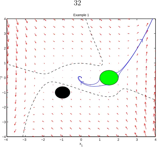
Consider the two-dimensional system (taken from [40, page 180])
˙
x1
˙
x2
=
x2
−x1 +13x31−x2
,
with X =R2. We want to verify that all trajectories of the system starting from the initial set X0 = {x ∈ R2 : (x1 −1.5)2 +x22 ≤ 0.25} will never reach the unsafe set
Xu = {x ∈ R2 : (x1 + 1)2 + (x2 + 1)2 ≤ 0.16}. Note that the system has a stable
focus at the origin and two saddle points at (±√3,0). SinceX0 contains a part of the
unstable manifold corresponding to the equilibrium (√3,0), the safety of this system cannot be verified exactly by computation of forward reachable sets in a finite time horizon.
For example, a polynomial barrier certificateB(x) that satisfies (2.2)–(2.4) is given by
B(x) = −13 + 7x21+ 16x22−6x21x22− 7
6x
4
1−3x1x32+ 12x1x2 −
12 3 x
3 1x2.
−4 −3 −2 −1 0 1 2 3 4 −4 −3 −2 −1 0 1 2 3 4 x 1 x2 Example 1
Figure 2.1: Phase portrait of the system in Section 2.4.1. Solid patches are (from left to right) Xu and X0, respectively. Dashed curves are the zero level set of B(x),
whereas solid curves are some trajectories of the system. The functionB(x) is strictly greater than zero for all x∈ Xu and strictly less than zero for all x∈ X0.
exhibiting the quadratic form −∂B
∂x(x)f(x) =Z(x)
TQZ(x), with
Q=
20 0 15 0 −15/2 −5
0 3 0 3/2 0 0
15 0 12 0 −6 −4
0 3/2 0 6 0 0
−15/2 0 −6 0 3 2 −5 0 −4 0 2 4/3
, Z(x) = x2 x2 2 x1
x1x2
x2 1x2
x3 1 .
In this case, the matrix Q is positive semidefinite, which implies the existence of a sum of squares decomposition for −∂B∂x(x)f(x) (and hence its nonnegativity). That (2.2)–(2.3) are satisfied can be shown by sum of squares arguments as well, and is also depicted pictorially in Figure 2.1. The zero level set of the barrier certificate separates Xu from all trajectories starting from X0. Hence, the safety of the system
x ′ = f 2(x,d) x 1 2+x 2 2+x 3 2≥ 0.03
x
1 2≤
5.12 x ′ = f
1(x,d) x 1 2 +0.01x 2 2 +0.01x 3 2≤ 1.01 0.99 ≤ x
1 2+0.01x
2 2+0.01x
3 2≤ 1.01
0.03 ≤ x
1 2+x
2 2+x
3 2≤ 0.05
CONTROL NO CONTROL
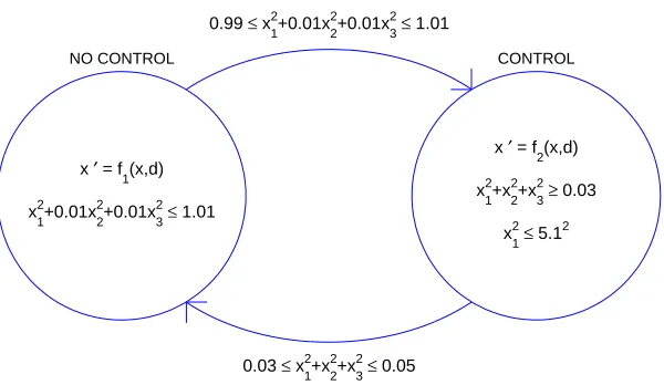
Figure 2.2: Discrete transition diagram of the system in Section 2.4.2. This system has two discrete locations: NO CONTROL and CONTROL, with the vector field and the invariant of each location depicted inside the corresponding circle. The texts labelling the transitions between locations describe the guard sets.
2.4.2
Hybrid System
Consider a hybrid system whose discrete transition diagram is depicted in Figure 2.2. The system starts in location 1 (NO CONTROL mode), with its continuous state initialized at Init(1) ={x∈R3 :x2
1+x22+x23 ≤0.01}. In this location, the continuous
state evolves according to ˙ x1 ˙ x2 ˙ x3 = x2
−x1+x3
x1+ (2x2+ 3x3)(1 +x23) +d
,f1(x, d),
until it reaches some point in the guard set Guard(1,2) = {x ∈ R3 : 0.99 ≤ x2 1 +
0.01x2
2+ 0.01x23 ≤1.01}, at which instance a controller whose objective is to prevent
|x1| from getting too big will be turned on, and the system jumps to location 2
(CONTROL mode). In location 2, the continuous dynamics is described by ˙ x1 ˙ x2 ˙ x3 = x2
−x1+x3
−x1 −2x2−3x3+d
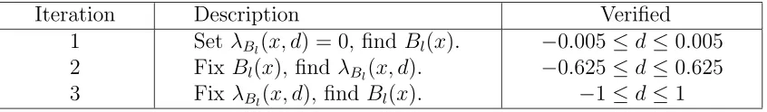
Iteration Description Verified 1 Set λBl(x, d) = 0, find Bl(x). −0.005≤d≤0.005
2 FixBl(x), find λBl(x, d). −0.625≤d≤0.625
3 FixλBl(x, d), find Bl(x). −1≤d≤1
Table 2.1: Description and results of the iterative method in Section 2.4.2. The third column indicates the disturbance range for which safety is verified.
The system will remain in this location until the continuous state enters the second guard set Guard(2,1) ={x∈ R3 : 0.03≤x2
1+x22+x23 ≤ 0.05}, where the controller
will be turned off and the system jumps to location 1. We assume nondeterminism in the jump from location 1 to location 2 and vice versa. For this system, the invariant of the discrete locations are given by I(1) ={x∈ R3 : x2
1+ 0.01x22 + 0.01x23 ≤ 1.01}
and I(2) ={x∈R3 :x2
1+x22+x23 ≥0.03, x21 ≤5.12}.
Our task in this example is to verify that |x1| never gets bigger than 5, if the
instantaneous magnitude of the disturbanced is bounded by 1. We define our unsafe sets as Unsafe(1) = ∅ and Unsafe(2) = {x ∈ R3 : 5 ≤ x1 ≤ 5.1} ∪ {x ∈ R3 :
−5.1≤x1 ≤ −5}, and compute a quartic barrier certificate satisfying the conditions
in Theorem 2.7. Using the iterative method described in Section 2.3.3 to enlarge the verifiable disturbance set, we obtain the results shown in Table 2.1. At the third iteration, we are able to prove the safety of the system.
2.4.3
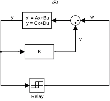
Limit of Design
.
In this example, we analyze the reachability of a linear system in feedback inter-connection with a relay. The block diagram of the system is shown in Figure 2.3, with the matrices A,B,C, and D given by
A=
0 1 0
0 0 1
−0.2 −0.3 −1
, B =
0 0 0.1
,
C =h 1 0 0 i
, D=h 0
i
y w
v
Relay K
x’ = Ax+Bu y = Cx+Du
Figure 2.3: Block diagram of the system in Section 2.4.3. We ask if it is possible to design a controller K that steers the system from an initial set X0 to a destination
setXu, subject to some other specifications.
and the relay element having the following characteristic:
w=
10, if y≥0,
−10, if y <0.
For the setsX ={x∈R3 :x2
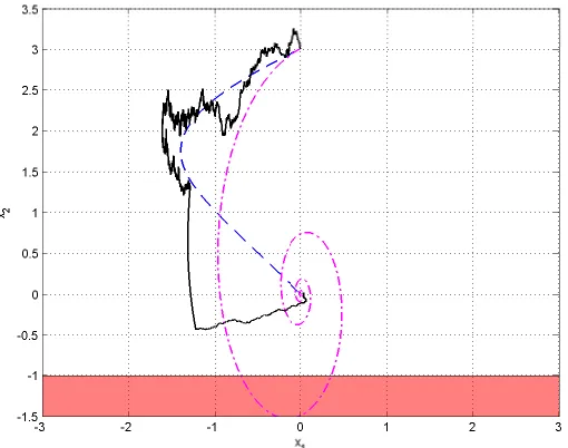
1+x22+x23 ≤42},X0 ={x∈R3 : (x1+2)2+x22+x23 ≤
0.12}, andXu ={x∈R3 : (x
1−2)2+x22+x23 ≤0.12}, we pose the following question:
Is it possible to design a controller K (possibly nonlinear and time-varying) with the
L2-gain not greater than one, which is connected to the system in the way shown in
Figure 2.3, such that the system can be steered fromX0 toXu while maintaining the state in X?
The requirement that the L2-gain of the controller is not greater than one can be
equivalently formulated as an integral quadratic constraint (IQC) [49] Z T
0
[y2(t)−v2(t)]dt ≥0 ∀T ≥0.
required conditions can be found. Hence we conclude that the given specification is impossible to meet.
2.5
Appendix: Non-Convex Conditions
In Section 2.1.2, it is mentioned that other non-convex conditions guaranteeing safety can be derived using viability theory. For example, using a viability theorem by Nagumo [55] and a characterization of contingent cone for a set described by inequal-ities [12], the following proposition can be obtained.
Proposition 2.18 Let the system x˙ =f(x) and the sets X ⊆Rn, X0 ⊆ X, Xu ⊆ X
be given, with the vector field f : Rn →Rn being locally Lipschitz continuous and X
being open. Suppose there exists a function B ∈ C1(Rn) that satisfies the following
conditions:
B(x)≤0 ∀x∈ X0, (2.42)
B(x)>0 ∀x∈ Xu, (2.43)
∂B
∂x(x)6= 0 ∀x∈ X such that B(x) = 0, (2.44) ∂B
∂x(x)f(x)≤0 ∀x∈ X such that B(x) = 0, (2.45)
then the safety of the system in the sense of Definition 2.1 is guaranteed.
Notice in particular that if there is no disturbance input, the vector field f(x) is locally Lipschitz continuous, and X is open, then the statement in Proposition 2.3 follows as a corollary of Proposition 2.18. We will now state some definitions and results needed to prove Proposition 2.18.
Definition 2.19 (Contingent Cone) LetX be a normed space,K be a non-empty
subset of X, and x belong to K. The (Bouligand) contingent cone to K at x is
TK(x) =
v ∈X : lim inf h→0+
dK(x+hv)
h = 0
where dK(y) is the distance of y to K, i.e., dK(y) = infz∈Kky−zk.
In proving Proposition 2.18, we will use X = Rn and K = {x∈ X : B(x) ≤0}. The contingent cone toK is characterized in the following lemma.
Lemma 2.20 (See, e.g., [12]) Let X = Rn and K = {x ∈ X : B(x) ≤ 0} for a continuously differentiable B(x). Then TK(x) = X if x is in the interior of K, and
TK(x) =
v ∈X : ∂B
∂x(x)v ≤0
for any x such that B(x) = 0, under the condition that ∂B
∂x(x)6= 0.
Theorem 2.21 (Nagumo5
) Let X be a finite dimensional vector space, K ⊆X be locally compact and f(x)be continuous from K toX. ThenK is locally viableunder
f(x), i.e., for any initial state x0 ∈K there existτ >0 such that at least one solution
x(t) of the differential equations x˙ = f(x) starting at x0 stays in K on [0, τ], if and
only if
f(x)∈TK(x) ∀x∈K.
Proof of Proposition 2.18. LetK be as defined in Lemma 2.20, and consider any initial condition x0 ∈∂K∩ X, where ∂K here denotes the boundary ofK. Since
f(x) ∈ TK(x) for all x ∈ K ∩ X, by Theorem 2.21 there is at least a trajectory of the system starting atx0 that on a small enough time interval is contained in K∩ X.
But in fact there is only one such trajectory, since in the proposition we assert that
f(x) is locally Lipschitz continuous, which guarantees uniqueness of solutions