Volume 2011, Article ID 501703,14pages doi:10.1155/2011/501703
Research Article
Channel Frequency Response Estimation for
MIMO Systems with Frequency-Domain Equalization
Yang Yang,
1Zhiping Shi,
2Yong Huat Chew,
3and Tjeng Thiang Tjhung
31Department of Electrical and Computer Engineering, Lehigh University, 19 Memorial Drive West, Bethlehem, PA 18015, USA 2National Key Laboratory of Communication, University of Electronic Science and Technology of China,
Chengdu 610054, Sichuan, China
3Institute for Infocomm Research, 1 Fusionpolis Way, #21-01 Connexis, Singapore 138632
Correspondence should be addressed to Yang Yang,[email protected]
Received 15 April 2010; Revised 24 October 2010; Accepted 2 December 2010
Academic Editor: Yeheskel Bar-Ness
Copyright © 2011 Yang Yang et al. This is an open access article distributed under the Creative Commons Attribution License, which permits unrestricted use, distribution, and reproduction in any medium, provided the original work is properly cited.
Since its recent adoption for the uplink transmissions in the next-generation cellular systems 3GPP long-term evolution (LTE) and LTE advanced, single-carrier frequency-domain equalization (SC-FDE), an effective technique to mitigate the distortion induced by long-spanning intersymbol interference has seen a surge of interest in the research community. Implementation of SC-FDE in multiple-input multiple-output (MIMO) systems usually requires, in advance, the channel information in terms of the channel frequency response (CFR). In this paper, we present a training-based CFR estimation scheme, which is hardware efficient when integrated with SC-FDE and space-time coding (STC) in MIMO systems. A thorough mean square error (MSE) analysis of this CFR estimation scheme is provided, where we consider linear estimators based on both least squares (LS) and minimum MSE (MMSE) criteria by assuming different knowledge of the channel statistics. More specifically, for the LS-based approach, we assume noa prioriknowledge of the channel statistics is given other than the noise statistics, while for the MMSE-based method, we assume both the channel covariance matrix and the noise statistics are known. Given a constraint which effectively limits the transmit power of training signals, we also investigate the optimal design of training signals under both criteria. For the special case when the number of transmit antennas is equal to 2, we further demonstrate that the CFR estimation could be implemented in an adaptive manner by means of certain block-wise recursive algorithms. Extensive simulation results are provided, which demonstrate the efficacy of this CFR estimation scheme.
1. Introduction
The severe frequency selectivity often characterizing wide-band radio channels would inevitably induce intersym-bol interference (ISI) which can span over many symintersym-bol intervals. High-speed broadband wireless systems targeting data rate of tens of megabits or beyond should be, as a result, designed to mitigate the effect of such intense ISI. Traditionally, time-domain equalization (TDE) is a popular approach to compensate for ISI in single-carrier communication systems. But for wideband channels, TDE becomes unattractive as its complexity grows exponen-tially with channel memory or it requires very long finite impulse response filters to achieve acceptable performance. An alternative approach is the single-carrier frequency-domain equalization (SC-FDE), which has the advantage
··· ··· ···
+ + TX 1
Block ST encoder Data
sequence
Training sequence
CP insertion
CP insertion
MIMO channel AWGN
AWGN CP removal
CP removal
FFT
FFT
FDE
IFFT
IFFT
CFR estimation Training
sequence Data sequence RX 1
TXNT RXNR
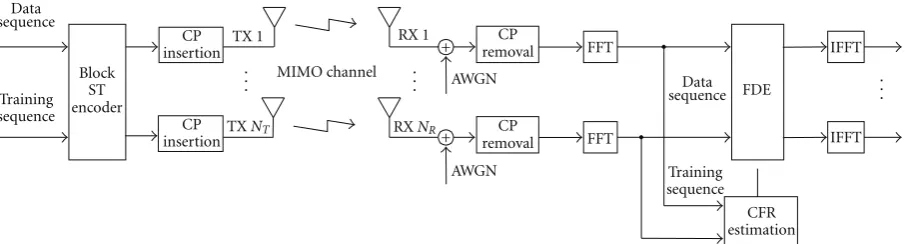
Figure1: Block diagram of the CFR estimation for MIMO system with STC and SC-FDE.
adopted for the uplink transmissions in the next-generation cellular systems 3 GPP long-term evolution (LTE) and LTE advanced [4]. SC-FDE has thus grasped more attention in both academic and industrial circles.
SC-FDE has also been applied to multiple-input multiple-output (MIMO) communication systems. This, however, is often done jointly with space-time coding (STC), in order that the spatial diversity available in a MIMO system can be exploited to further mitigate the frequency selectivity, for example, [5–9]. For this case, properly designed ST block codes (STBCs) are generally required and there exist some works in that regard. For example, a time-reversal Alamouti-like STBC scheme with FDE was proposed firstly in [5]. This scheme is attractive as it can achieve full spatial diversity, and nearly full transmit rate if the cyclic prefix (CP) overhead is ignored. For SC-FDE in MIMO systems with more than 2 transmit antennas, a general block-level STC was proposed in [6] and a method based on quasi-orthogonal STBCs was proposed in [7].
Note that when performing FDE in MIMO systems, the channel frequency response between each transmit-receive antenna pair is usually required at the receiver to recover the transmitted signals [2,3]. To obtain such channel frequency response (CFR) knowledge, one approach is to obtain the channel impulse response (CIR) firstly and then transfer it back to the frequency domain through FFT processing. As a result, the CFR estimation problem merely reduces to the problem of estimating the CIR in MIMO systems, which has been vigorously investigated over the years, for example, see [10] and references therein. As an alternative, one can apply the FFT firstly, and then estimate the CFR directly afterwards. In fact, we notice that this alternative approach, or the CFR estimation problem, has been studied, for example, in [11] for systems with single transmit and single receive antenna, and in [12] for SC-FDE in ultra-wideband communication systems. However, there does not seem to exist a lot of works which explore this alternative approach particularly for MIMO systems employing both STC and SC-FDE. This line of work merits interest on its own terms, for not only can it advance the existing knowledge on the subject of CFR estimation, but the CFR estimation scheme, when designed in a manner to be integrated with the techniques of STC and FDE in MIMO systems, can be amenable to system implementation, and has the potential
to induce less hardware complexity and cost. This basically motivates our work as detailed next.
In this paper, we present and investigate a CFR estimation scheme for MIMO systems with both STC and FDE. In this scheme, training sequences are encoded in space and time in a similar manner as data sequences. (We notice that the CIR estimation for MIMO channels using ST codes was consid-ered in [13,14].) In fact, the same set of coding hardware can be reused; thus, no additional hardware complexity is introduced at the transmitter and this is particularly suitable for mobile terminals. At the receiver, different from the tradi-tional approach where CIR is obtained first then transferred to CFR, these training sequences are simply processed in a similar fashion as the data sequences, for example, CP removal and FFT processing. Following these procedures, estimation of the CFR can thus be done directly in the frequency domain. As the CFR estimation can make use of the existing FFT modules for FDE, fewer complexity or cost would be required at the receiver. This scheme is illustrated in
Figure 1. Further, in this paper, we provide a thorough mean square error (MSE) analysis for the CFR estimation based on two criteria, least squares (LS) and minimum MSE (MMSE), by assuming different a priori knowledge of the channel statistics. More specifically, for the LS-based approach, we assume noa prioriknowledge of the channel statistics is given other than the noise statistics, while for the MMSE-based method, we assume both the channel covariance matrix and the noise statistics are known. Under both criteria, we also study the optimal training sequence design by imposing a constraint on the transmit power of training sequences. Finally, we investigate the adaptive implementation of the proposed CFR estimation scheme for Alamouti-like trans-missions. We provide several block-wise recursive algorithms to update the adaptive filter, and also study the convergence behaviors of these recursive algorithms.
this special case, and provide a brief convergence analysis. In
Section 5, we provide extensive simulation results and also compare with others’ work to demonstrate the efficacy of this estimation approach.Section 6concludes this paper.
Notation. Throughout this paper, we use bold upper case letters to denote matrices and bold lower case letters to signify column vectors. Superscript {·}H, {·}∗, and {·}T will be used to denote the complex conjugate transpose, conjugate, and transpose of a matrix or vector, respectively. We use diag{a}for a diagonal matrix with its diagonal vector given by a, and ⊗ for Kronecker product. IK denotes the identity matrix of sizeK×K, and0M×N for a zero matrix of size M ×N. We use the subscript {·}F to denote the
matrices or vectors in the frequency domain, and (·)+for the nonnegative part of a real-valued scalar or matrix.
2. Signal and System Model
We consider an ST-coded MIMO system equipped with NT transmit and NR receive antennas. With symbol rate sampling, let h(p,q) = [h(p,q)(0),. . .,h(p,q)(ν)]T denote the
equivalent baseband discrete-time CIR (including the trans-mit and receive filters as well as the multipath effect) between thepth transmit antenna and theqth receive antenna, where 1 ≤ p ≤ NT, 1 ≤ q ≤ NR, and ν is the channel order. We assume the channel is quasistatic, that is, its response remains time invariant within one ST-coded frame but can vary from frame to frame. We defineNSvectors of dimension
L×1,{si}NS
i=1as the training sequences, where the symbols
in si belong to the same alphabet A, and L denotes the sequence length and is assumed to be at least equal to the number of multipaths, that is,L ≥ν+ 1. In this proposed CFR estimation scheme, the training sequencesiis encoded in space and time, using the same ST block encoder for data sequences, as depicted in Figure 1. As a result of this, the same set of hardware can be reused without additional complexity and cost. As for the ST encoder, we adopt the code design described in [6]. It is an extension of the original orthogonal STBCs in [15,16] for frequency-selective fading channels. This type of STBCs are capable of achiev-ing full spatial diversity and are particularly amenable to FDE.
Without loss of generality, suppose theNStraining blocks are ST coded in a manner that they are transmitted overNc= 2NStime slots, where a time slot is defined as the duration required to transmit a CP appended training block. Thus, the code rate is given byR=NS/Nc=1/2. There exist some sporadic code designs which could achieve code rate higher than 1/2. For example, whenNT =3 and 4, the code design withR = 3/4 can be found in [16]. However, it has been proved in [17] that with complex signal constellation and under the orthogonality assumption, R cannot be greater than 3/4 forNT >2. For simplicity, in this part we only focus on the case ofR=1/2 forNT >2. The special case ofR=1 forNT=2 will be discussed in detail inSection 4.
Let {Πi}NS
i=1 be a set of NS ×NT real-valued matrices of a full-rate generalized orthogonal STBC design for real
symbols. Entries of Πi are either 0 or ±1, and Πi further satisfies the following conditions [18, Chapter 7]:
ΠT
iΠi=INT, ΠT
iΠj= −ΠTjΠi, i /=j.
(1)
Then, for the block-level generalized complex orthogonal STBC that is employed in our work, the code matrix, if denoted asG∈CNcL×NT, can be written as
G= NS
i=1
ΓAi⊗si+ΓBi⊗P (1)
L s∗i
, (2)
where ΓAi and ΓBi are both Nc × NT matrices, and are, respectively, defined as
ΓAi= ⎡ ⎣ Πi
0NS×NT ⎤
⎦, ΓB
i= ⎡ ⎣0NS×NT
Πi
⎤
⎦. (3)
In (2),P(1)L is anL×Lpermutation matrix which performs a reverse cyclic shift when applied to an arbitraryL×1 vector, for example, supposes= [s(0),s(1),. . . s(L−1)]T, we then have
P(1)L s∗=[s∗(0),s∗(L−1),s∗(L−2),. . .,s∗(1)]T. (4) Given the properties ofΠiin (1), it can be easily verified that ΓAiandΓBihave the following properties:
ΓT
AiΓAi=INT, ΓTBiΓBi=INT, ΓT
AiΓAj = −ΓTAjΓAi, ΓTBiΓBj = −ΓTBjΓBi, i /=j,
ΓT
AiΓBj =0NT×NT, ∀i,j.
(5)
LetG(:,i) denote theith column ofGthat corresponds to the training blocks to be transmitted from theith transmit antenna overNc time slots. For notational convenience, we express theith column ofGas follows:
G(:,i)= NS
m=1
Γ(:,i)⊗sm+Γ(:,i)⊗P(1)L s∗m
= sT
i(1),sTi(2),. . .,sTi(Nc)
T
,
(6)
wherei=1,. . .,NT. To give an example ofG, let us consider a code design with rateR =1/2 forNT =3, whereNS=4 andNc=8. For this instance,Gis illustrated as below
G= ⎛ ⎜ ⎜ ⎜ ⎜ ⎜ ⎜ ⎜ ⎜ ⎜ ⎜ ⎜ ⎜ ⎜ ⎜ ⎜ ⎜ ⎜ ⎜ ⎜ ⎜ ⎝
s1 s2 s3
−s2 s1 −s4
−s3 s4 s1
−s4 −s3 s2
P(1)L s∗1 P(1)L s∗2 P(1)L s∗3
−P(1)L s∗2 P(1)L s∗1 −P(1)L s∗4
−P(1)L s∗3 PL(1)s∗4 P(1)L s∗1
−P(1)L s∗4 −P
(1)
L s∗3 P (1)
L s∗2 ⎞ ⎟ ⎟ ⎟ ⎟ ⎟ ⎟ ⎟ ⎟ ⎟ ⎟ ⎟ ⎟ ⎟ ⎟ ⎟ ⎟ ⎟ ⎟ ⎟ ⎟ ⎠ = ⎛ ⎜ ⎜ ⎜ ⎜ ⎜ ⎜ ⎜ ⎜ ⎜ ⎜ ⎜ ⎜ ⎜ ⎜ ⎜ ⎜ ⎜ ⎜ ⎝
s1(1) s2(1) s3(1)
s1(2) s2(2) s3(2)
s1(3) s2(3) s3(3)
s1(4) s2(4) s3(4)
s1(5) s2(5) s3(5)
s1(6) s2(6) s3(6)
s1(7) s2(7) s3(7)
After ST coded, the transmission structure of the training sequences is shown inTable 1.
To avoid the interblock interference from preceding information or training sequences, a CP with a length of
ν is inserted for each block before transmission. Then, at time slotk, the training sequencesp(k) is forwarded to the
pth transmit antenna after CP insertion. The length of total training symbols from each transmit antenna, denoted as Nb, is equal toNb =Nc(L+ν), and its minimum length is Nb=Nc(2ν+ 1) whenLis chosen to be equal toν+ 1.
3. CFR Estimation for
MIMO Transmissions
(
N
T>
2)
At the receiver, symbols corresponding to the CP are discarded. Thus, the received signal at theqth receive antenna at time slotkcan be written as
xq(k)
= NT
p=1
H(p,q)sp(k) +nq(k), q=1,. . .,NR, k=1,. . .,Nc,
(8)
whereH(p,q)is anL×Lchannel matrix with its (k,l)th entry
given byh(p,q)((k−l) mod L), andn
q(k) denotes the additive white Gaussian noise (AWGN) vector. It is easy to verify that H(p,q)is a circulant matrix. Thus, its eigen matrix is the FFT
matrix, or in other words, its eigendecomposition can be written as
H(p,q)=FH L ·diag
h(Fp,q)·FL. (9)
FL is the orthonormal FFT matrix whose (k,l)th entry is given by
FL(k,l)= 1 √
Lexp
−j2π(k−1)(l−1)
L
, (10)
where k = 1,. . .,Land l = 1,. . .,L. If denotingD(Fp,q) = diag(h(Fp,q)), we have
D(Fp,q)(i,i)=h(Fp,q)(i)=ν k=0
h(p,q)(k)e−j2πk(i−1)/L, (11)
where i = 1,. . .,L. Applying the FFT operations on both sides of (8), we obtain
xqF(k)=
NT
p=1
D(Fp,q)spF(k) +nqF(k), (12)
wherexqF(k)=FLxq(k),spF(k)=FLsp(k), andnqF(k)=
FLnq(k).
SinceD(Fp,q)is diagonal, we can rewrite (12) into
xqF(k)=
NT
p=1
SpF(k)hF(p,q)+nqF(k), (13)
Table1: Transmission structure of training sequences (NT>2).
1 · · · Nc
TX 1 s1(1) · · · s1(Nc)
..
. ... ... ...
TXNT sNT(1) · · · sNT(Nc)
where SpF(k) = diag{spF(k)}. Stacking Nc blocks of received signals at theqth receive antenna, we have
⎡ ⎢ ⎢ ⎢ ⎢ ⎣
xqF(1) .. . xqF(Nc)
⎤ ⎥ ⎥ ⎥ ⎥ ⎦
xqF =
⎡ ⎢ ⎢ ⎢ ⎢ ⎣
S1F(1) · · · SNTF(1)
..
. . .. ...
S1F(Nc) · · · SNTF(Nc)
⎤ ⎥ ⎥ ⎥ ⎥ ⎦
SF
×
⎡ ⎢ ⎢ ⎢ ⎢ ⎢ ⎣
h(1,Fq) .. . h(NT,q)
F ⎤ ⎥ ⎥ ⎥ ⎥ ⎥ ⎦
hqF
+
⎡ ⎢ ⎢ ⎢ ⎢ ⎣
n1F(1)
.. . nqF(Nc)
⎤ ⎥ ⎥ ⎥ ⎥ ⎦
nqF
(14) or in a more simplified form
xqF =SFhqF +nqF. (15)
Collecting the received signals across all those NR receive antennas, we obtain the received data matrix XF = [x1F,. . .,xNR
F ], which is expressed as
XF =SFHF +NF, (16)
whereHF =[h1
F,. . .,hNFR] andNF =[n1F,. . .,nNFR]. Thus,
our task is to recover the CFRHF from (16). Additionally, let us denote hq = [h(1,q)T
,. . .,h(NT,q)T]T
as the corresponding CIR associated with theqth antenna, and stack all the CIR acrossNR receive antennas in matrix
H=[h1,. . .,hNR]. We further define the compound inverse
FFT (IFFT) matrix FH
NT = INT ⊗FHL, and the compound transmit matrixTNT=INT⊗[Iν+1|0(ν+1)×(L−ν−1)]. Therefore,
the corresponding CIR estimate can be computed by
H=√1
LTNTF
H
NTHF, (17)
where HF is the CFR estimate for HF. In the sequel, we discuss the linear CFR estimators based on both LS and MMSE criteria, along with the respective optimal designs of training sequences.
3.1. LS Estimator with Power Constraint. For the convenience of ensuing analysis, we explicitly make the following assump-tion.
(A1) All noise components are assumed to be com-plex, independently and identically Gaussian dis-tributed with zero mean and variance σ2
we have nqF ∼ CN(0NcL×1,σ 2
nINcL) and NF ∼
CN(0NcL×NR,σ 2
nNRINcL).
Except for the noise statistics, we assume noa priori knowl-edge of the channel parameters (e.g., the covariance matrix of the CFR) is given, and we only consider the conventional LS method. Therefore, the unique LS solution HF that minimizes the cost function defined byXF −SFHF2can be written as
HF =SH
FSF −1
SH
FXF. (18)
It should be noted that if we want to obtain the CFR with a length greater than the default lengthL, interpolation is needed.
Based on assumption (A1), it is clear that this estimate is unbiased since E{HF} = HF. Let us define the CFR estimation error as EF = HF −HF. Using (16) and (18), we obtain
EF =
SH
FSF −1
SH
FNF. (19)
Its correlation matrix,REF = E{EFEHF}, can be calculated through
REF =σ2
nNR
SH
FSF −1
. (20)
Thus, the MSE for this CFR estimation is given by
EEF2=trRE F
=σ2
nNR·tr
SH
FSF −1
. (21)
Now we consider the problem of designing the matrix
SF so that the estimation error is minimized. To have a reasonable solution, it is necessary to impose a constraint to limit the power of training sequences. Let such a constraint be SF2 ≤ P0, where P0 is a given constant. Note that
the power used in the cyclic prefix is not included in this formulation. Mathematically, this power constraint can also be written as tr{SH
FSF} ≤ P0. For simplicity, we start
with a general problem formulation, without examining the structure of the data matrix SF but only assuming it has full rank. Therefore, our task is to findSF that minimizes the MSE subject to the power constraint given above. This constrained optimization problem can be cast as
min SF
trSH
FSF −1
,
s.t. trSFHSF
≤P0.
(22)
To solve this problem, the following lemma will be useful.
Lemma 1. For any M ×M positive semidefinite Hermitian matrix A with its (i,j)th entry given by ai j, the following
inequality holds
tr A−1!≥ M
i=1
1
aii
, (23)
where the equality is achieved if and only ifAis diagonal.
Applying this lemma and the method of Lagrange multipliers [19], we could readily solve this optimization problem. For brevity, we omit the details and simply provide the solution
SH
FSF = P0
NTL
INTL, (24)
which means that the diagonal entries of SFHSF have the same value. Re-examining the matrix SF as defined in (14) and its relation to G in (2), we find that due to the orthogonal structure of the ST code, SH
FSF is precisely
diagonal. Moreover, recall{si}NS
i=1are training sequences, we
definesiF = FLsi and SiF = diag{siF} fori = 1,. . .,NS. Then, we arrive at the following result.
Theorem 1. The following equality holds
SH
FSF =INT⊗ ⎧ ⎨ ⎩2
NS
i=1
SHiFSiF
⎫ ⎬
⎭. (25)
Proof. SFHSF is anNTL×NTLmatrix and can be expressed in the block matrix form as
SH
FSF = ⎛ ⎜ ⎜ ⎜ ⎜ ⎝
Ξ1,1 · · · Ξ1,NT
..
. . .. ...
ΞNT,1 · · · ΞNT,NT
⎞ ⎟ ⎟ ⎟ ⎟
⎠, (26)
whereΞi,j,i =1,. . .,NT, j =1,. . .,NT, is a square matrix of size L×L. According to both (6) and (14), Ξi,j can be expressed as
Ξi,j=
(
INc⊗FL !
·G(:,i))H( INc⊗FL
!
·G :,j!)
= ⎧ ⎨ ⎩ Ns
m=1
ΓT
Am(:,i)⊗S
H
mF +ΓTBm(:,i)⊗SmF ⎫⎬ ⎭ × ⎧ ⎨ ⎩ Ns
n=1
ΓAn :,j !
⊗SnF +ΓBn :,j
!
⊗SH
nF
⎫⎬ ⎭.
(27)
To simplify (27), we need to use the mixed-product propertyof Kronecker product, that is, (A⊗B)(C⊗D) = AC⊗BD, whereA,B,C, andDare matrices of such size that one can form the matrix productsACandBD. Further, given the properties ofΓAmandΓBnin (5), we have the following:
ΓT
Am(:,i)ΓAn :,j ! = ⎧ ⎪ ⎪ ⎪ ⎪ ⎨ ⎪ ⎪ ⎪ ⎪ ⎩
1, m=n, i=j, 0, m=n, i /=j,
−ΓT
An(:,i)ΓAm :,j !
, m /=n.
(28)
Similar properties also hold forΓTBm(:,i)ΓBn(:,j). Moreover,
we have ΓT
Am(:,i)ΓBn :,j !
=ΓT
Bm(:,i)ΓAn :,j !
=0, ∀i,j,m,n.
Based on the above properties, (27) can be simplified into
Ξi,j=
⎧ ⎪ ⎪ ⎨ ⎪ ⎪ ⎩
2 NS
i=1
SH
iFSiF, i= j,
0, i /=j.
(30)
Plugging (30) into (26), we then obtain (25).
Based on (24) and (25), we summarize the following result.
Theorem 2. The optimal training signals under the LS criterion should satisfy the following condition:
NS
i=1
SHiFSiF =2P0
NTL
IL. (31)
This condition is the same as
NS
i=1
++siF j!++2
= P0
2NTL
, ∀j∈[1,L], (32)
wheresiF(j)denotes thejth element ofsiF.
Of note is that althoughTheorem 2states the conditions for training signals to be optimal in the sense of achiev-ing the minimum value of MSE, it does not mean any sequences which satisfy (32) would be suitable for practical applications. This is because practical implementation of communication systems will inevitably impose some addi-tional constraints on the sequences. To give an example, let us consider the CP-based communication systems. These systems are usually plagued by the well-known peak-to-average ratio (PAR) problem; thus, sequences with lower PAR values are, in general, more preferred in practice, for they can greatly alleviate the requirement on the power amplifier. Under this circumstance, training sequences which not only satisfy (32) but have a constant magnitude in both the time domain and the frequency domain would lend themselves to be a superior choice, for they are able to successfully preclude the PAR problem while achieving the minimum value of MSE. Chu sequences [20] and the class of training sequences proposed in [21] are examples of those sequences. Finally, the resulting minimum value of MSE can be calculated by
EEF2=L
j=1
NTNRσn2 2,NS
i=1++siF j!++2
=σn2NR(NTL)2
P0 . (33)
3.2. MMSE Estimator with Power Constraint. In this section, we consider the linear MMSE estimation of the CFR as well as the optimal training sequence design. For simplicity, we consider only the CFR associated with the qth receive antenna, that is, hqF, which was defined in (14). Besides assumption (A1), we make one additional assumption about the channel statistics as follows.
(A2) The CFRhqF is a Gaussian random vector with zero mean and full-rank covariance matrixΣq.
For convenience, we denoteΣqbyΣ. SincehqF =(INT⊗FL)hq,
we have
Σ= INT⊗FL !
·Ehq(hq)H·I
NT⊗FHL
, (34)
where E{hq(hq)H} is the covariance matrix of the corre-sponding CIR.
The MMSE estimate of the CFR can be computed through
hqF =SH
FSF +σn2Σ−1
−1 SH
FxqF. (35)
We define the CFR estimation error aseqF =hqF −hqF, then the resulting MSE can be expressed as
E---eqF---2
=trσ−2
n SFHSF +Σ−1
−1
. (36)
Similar to the approach that we took inSection 3.1, we also impose a power constraint, and the design problem can be formulated into
min SF tr
σn−2SFHSF +Σ−1−1
s.t. trSFHSF
≤P0.
(37)
Note thatΣ can be diagonalized through its eigenvalue decomposition, that is,
Σ=VΛVH, (38)
whereVis a unitary matrix whose columns are eigenvectors ofΣ, andΛis a nonnegative and diagonal matrix consisting of all the eigenvalues ofΣ. Then, (36) can be reformulated into
E---eqF---2
=trσ−2
n ΨHΨ+Λ−1
−1
, (39)
whereΨ=SFVis anNcL×NTLmatrix. AsVis unitary, it follows tr{SH
FSF} = tr{ΨHΨ}. According toLemma 1, the
minimum value of E{eqF2}is attained when (σ−2
n ΨHΨ+ Λ−1) is diagonal. Let Q = ΨHΨ, then Q must be a diagonal matrix with elementsQii ≥ 0, fori =1,. . .,NTL. Consequently, we can reformulate the optimization problem into
min Q tr
σ−2
n Q+Λ−1
−1
,
s.t. tr{Q} ≤P0.
(40)
Using the method of Lagrange multipliers [19], we can obtain the following solution to the modified optimization problem
Qii=
.
τ− σ
2
n Λii
/+
, ∀i∈[1,NTL], (41)
whereΛiidenotes the (i,i)th element ofΛ, and the value ofτ
can be found by solving NTL
i=1 .
τ− σn2 Λii
/+
Alternatively,Qcan be rewritten as
Q=τINTL−σ 2
nΛ−1
+
. (43)
Thus, the resulting MSE can be computed through
E---eqF---2
= NTL
i=1
Λii Λiiσ−2
n τ−1
!+
+ 1. (44)
It is worth noting that ΨHΨ is invariant to the post-multiplication of Ψ by a semi-orthogonal matrix. Thus, given the optimal solution forQin (43), a general solution for Ψ can be composed as Ψ = ZQ1/2, where Z is an
NcL×NTLmatrix with its column forming an orthonormal basis. SinceΨ=SFV, it is clear that the necessary condition
forSF to be optimum isSF = ZQ1/2VH. Meanwhile, we haveSFHSF =VQVH and both sides are diagonal matrices. Considering the structure of SF in (14) and applying
Theorem 1, we are thus led to following result.
Theorem 3. The optimal training signals under the MMSE criterion should satisfy the following condition for a specific channel statistics (i.e.,Σ)
V·τINTL−σ 2
nΛ−1
+
·VH=I
NT⊗ ⎡ ⎣2NS
i=1
SH iFSiF
⎤ ⎦. (45)
Equation (45) specifies the essential characteristics of the optimum sequence under the MMSE criterion. It indicates that the optimal design should employ a water-filling type power allocation. Evidently, the structure of the covariance matrix Σwill have a large impact on the optimal training signal design. For example, when Σis diagonal, then from (34), we can see that E{hq(hq)H} can be a block circulant matrix, and the optimum condition (45) would represent a water-filling in power distribution with respect to the power spectral density samples of the CIR. For this special case, the optimal sequence may be generated through the frequency-domain water-filling. For cases whereΣis not diagonal, the optimal condition (45) may need to be jointly considered with the Kronecker product approximation in [22]. We omit further discussions for brevity.
4. CFR Estimation for
Alamouti-Like Transmissions
Here, we study the CFR estimation for the special case of NT = 2 and NR = 1. This corresponds to the Alamouti-type transmission, where NS = Nc = 2 and R = 1. The transmission structure for the training sequences is illustrated in Table 2. The length of total training symbols from each transmit antenna,Nb, is equal toNb =2(L+ν), and its minimum length isNb=4ν+2 whenLis chosen to be the minimum valueν+ 1. At the receiver, CPs are removed, which yields the channel input-output relationship in matrix vector form as
x1(k)=H(1,1)s1+H(2,1)s2+n1(k),
x1(k+ 1)= −H(1,1)P(1)L s∗2 +H(2,1)P (1)
L s∗1 +n1(k+ 1),
(46)
Table2: Transmission structure of training sequences (NT=2).
time slotk time slotk+ 1 TX1 s1(k)=s1 s1(k+ 1)= −P(1)L s∗2
TX2 s2(k)=s2 s2(k+ 1)=P(1)L s∗1
wherex1(k) andx1(k+ 1) denote two consecutive received
blocks at the single receive antenna. Applying the orthonor-mal FFT matrixFLon (46), we obtain the frequency domain input-output relationship as shown below
⎡
⎣ x1F(k)
x1F(k+ 1) ⎤ ⎦=
⎡
⎣ S1F S2F
−S∗2F S∗1F
⎤ ⎦ ⎡ ⎣h
(1,1) F
h(2,1)F
⎤ ⎦+
⎡
⎣ n1F(k)
n1F(k+ 1) ⎤ ⎦.
(47) For this special case, the CFR estimation based on both the LS and MMSE criteria can be readily obtained by following the procedures outlined inSection 3. In this section, we further demonstrate that the CFR estimation for this special case can be implemented adaptively with block-wise recursive algorithms. Additionally, we also provide a brief convergence analysis of these algorithms.
4.1. Adaptive Implementation of CFR Estimation. It is easy to show that the CFR estimator for this special case has the following structure
GF =
⎡
⎣G1F −G2F
GH2F GH1F ⎤
⎦, (48)
where G1F and G2F are both L× L diagonal
matri-ces. Consider the LS estimator as an example, we have G1F = [SH1FS1F +SH2FS2F]−1SH1F and G2F =
[SH1FS1F +SH2FS2F]
−1
S2F. Now let us define the diagonal
vectors of G1F and G2F asg1F and g2F, respectively, that
is,G1F =diag{g1F}andG2F = diag{g2F}. Then, we can
write the CFR estimate as
⎡ ⎣h1F
h2F ⎤ ⎦
hF
=
⎡
⎣G1F −G2F
GH2F GH1F
⎤ ⎦
GF ⎡
⎣ x1F(k)
x1F(k+ 1) ⎤ ⎦
xF .
(49)
We further define L × L diagonal matrices X1F(k) =
diag{x1F(k)}andX1F(k+ 1)=diag{x1F(k+ 1)}. Then, (49)
can be reformulated into
⎡ ⎣g1F
g2F ⎤ ⎦
gF
=
⎡
⎣ Φ·X1HF(k) Φ·X1F(k+ 1)
−Φ·XH
1F(k+ 1) Φ·X1F(k) ⎤ ⎦
UF
⎡ ⎣h1F
h∗2F
⎤ ⎦
˘
hF
(50) or the simplified form
gF =UFh˘F, (51)
where in (50),Φ = [XH
1F(k)X1F(k) +X1HF(k+ 1)X1F(k+
the size of 2L×2L;gF is a 2L×1 vector that contains the elements ofg1F andg2F.
We would like to emphasize that this reformulation from (49) to (50) is largely attributed to the benign property of Alamouti’s code. This, as a result, enables the CFR estimation to be performed adaptively, and the channel to be tracked when the adaptive filter operates. To be more specific, we can viewUF as the tap-input data matrix,gF as the output, and ˘hF as the filter coefficients. The block diagram of this adaptive filter is depicted inFigure 2. We further define the error signal ˘eF, which is generated by comparing the filter output with the desired response, that is,
˘
eF =gF −UFh˘F. (52)
Note that as gF is fixed and already available beforehand at the receiver, the adaptive filter can always operate at the training mode. Hence, if the channel is slowly time-varying, the adaptive method, through estimating the current channel gains based on the previous channel estimate, can achieve accuracy refinement without significantly increasing the complexity. Simulation results illustrating this can be found inSection 5. For notational convenience, we add in the time index for vectors or matrices in the ensuing description. And we summarize the recursive algorithms that are used to update the CFR estimate inTable 3, which include the block least mean square (LMS) algorithm and the block recursive least squares (RLS) algorithm.
The block RLS algorithm usually achieves a quicker convergence than the block LMS algorithm (as will be shown later by simulation results). But such a quick convergence is attained at the cost of a heavy increase in the computational complexity. To exemplify this, let us examine the computa-tional complexity of both algorithms. At each iteration, the block LMS algorithm requires aroundO(8L) computations, while the block RLS algorithm requires O(24L3 + 20L2 +
4L) operations. A fast version of this block RLS algorithm, namely fast subsampled-updating RLS algorithm [23], can be used to achieve some complexity reduction, but may make this filter cumbersome. Fortunately, thanks to the special structure of the Alamouti’s code, it is easy to verify that UH
F(k)UF(k)=I2L. Furthermore, we can induce thatP(k) (cf.Table 3) is a 2L×2Ldiagonal matrix, that is,P(k) = I2⊗P(k), where P(k) denotes an L×L diagonal matrix.
Then, by following a similar technique used in [24,25], we can avoid the need for matrix inversion in the block RLS algorithm and hence can eventually achieve a substantial reduction in the computational complexity but without losing the convergence advantage. For brevity, we summarize the simplified algorithm inTable 4. This simplified algorithm requires onlyO(13L) operations for each iteration, which is much less than that of the original block RLS algorithm.
It is worthwhile to make a remark here that the above adaptive implementation of the CFR estimation is a special property owned by the Alamouti scheme withNT=2. When NTincreases beyond 2, the linear CFR estimatorGF, under
both the LS and MMSE criteria (cf. (18) and (35)), will no longer have the simple Alamouti’s structure. And so, a similar transformation as that from (49) to (50) may not necessarily
Table3: Adaption algorithms for Alamouti-like transmissions.
Block LMS algorithm Computation: fork=2, 4,. . ., compute ˘
eF(k−2)=gF(k−2)−UF(k−2) ˘hF(k−2) ˘
hF(k)=h˘F(k−2) +μUHF(k−2)˘eF(k−2)
whereμdenotes the step size.
Block RLS algorithm Initialize the algorithm by setting
˘
hF(0)=0,
P(0)=δ−1I
2L.
δis a small positive constant andλis the forgetting factor (λ <1). For each instant of time,k=2, 4,. . ., compute
C(k)=P(k−2)UH F(k)
V(k)=λI2L+UHF(k)C(k)
K(k)=C(k)·V−1(k) P(k)=λ−1[P(k−2)−K(k)U
F(k)P(k−2)]
˘
eF(k)=gF(k)−UF(k) ˘hF(k−2)
˘
hF(k)=h˘F(k−2) +P(k)UHF(k)˘eF(k)
Table4: Simplified block RLS algorithm.
Initialize the algorithm by setting ˘
hF(0)=0, P(0)=δ−1I
L.
δis a small positive constant andλis the forgetting factor (λ <1). For each instant of time,k=2, 4,. . ., compute
Ω(k)=[λIL+P(k)]−1
P(k)=λ−1[P(k−2)−P(k−2)Ω(k)P(k−2)]
˘
eF(k)=gF(k)−UF(k) ˘hF(k−2)
˘
hF(k)=h˘F(k−2) + [I2⊗P(k)]UHF(k)˘eF(k)
hold. Then, the adaptive implementation for CFR estimation for cases ofNT >2 requires further investigation.
4.2. Convergence Analysis. Convergence behaviors of these block-level recursive algorithms are briefly discussed as follows. We are interested in the behavior of ξ(k) = E{e˘F(k)˘eH
F(k)}, particularly at the steady state, where ˘eF(k)
denotes the error signal, as defined in (52). For the block LMS algorithm, we define the weight-error vector as
vF(k)=h˘F(k)−hF
,0, (53)
wherehF,0is the optimum tap-weight vector for the filter.
Thus, we have
vF(k)=vF(k−2) +μUHF(k−2)˘eF(k−2). (54)
DefiningeF,0(k)=gF(k)−UF(k)hF,0, we have
˘
eF(k)=eF,0(k)−UHF(k−2)vF(k). (55)
Let the weight-error correlation matrix be given as
Rvv(k)=EvF(k)·vH
F(k)
Construct data matrix
Adaptive algorithm
+ −
∑
x1F (k)
x1F (k+ 1)
UF(k)
˘
hF (k)
˘
eF (k) g1F (k)
g2F (k)
Figure2: Block diagram of the adaptive filter.
Thus, the MSE of weight vector error can be obtained by simply taking the trace of Rvv(k). To facilitate the convergence analysis, we make the following assumptions.
(A3) Elements of eF,0(k) are samples of a white noise
process, which implies that E{eF,0(k)eHF,0(k)} = ξmin·I2L, whereξminis the minimum MSE at the filter
output.
(A4)UF(k) and eF,0(k) are jointly Gaussian, and are
uncorrelated with each other.
(A5)vF(k) is independent ofUF(k) andeF,0(k). Further,
we assumeRuu=E{UHF(k)UF(k)}/2L, whereRuuis the correlation matrix of the filter tap inputs.
Based on the above assumptions and following a similar procedure in [26, Appendix 8A], we can compute theexcess MSE, which is defined as the difference between the steady-state MSE (i.e.,ξ(k= ∞)) and the minimum MSEξminof an
adaptive filter, approximately by
ξexcessBLMS=μξ min
2 tr(Ruu), (57) where tr(Ruu) is equivalent to the sum of the powers of the signal samples at the filter tap inputs. Accordingly, the
misadjustment, a dimension-free degradation measure that is defined as the ratio of the steady-state value of the excess MSE to the minimum MSE, can be written as
MBLMS=μ
2tr(Ruu). (58) Also, the steady-state MSE of the block LMS algorithm is given by
ξsteadyBLMS=2Lξmin+μξmin
2 tr(Ruu). (59) It is obvious that the convergence behavior of the block LMS algorithm is governed by the eigenvalues of the correlation matrixRuuof the filter tap input. Therefore, similar to the
conventional LMS algorithm, the block LMS algorithm in nature is also a stochastic implementation of the steepest-descent method[26].
For the block RLS algorithm, its convergence analysis is undertaken on an adaptive identification scheme [27]. We consider a linear multiple regression model characterized by
gF(k)=UF(k)hF,0+eF,0(k), (60)
wherehF,0is the regression parameter vector,UF(k) is the
tap-input matrix, eF,0(k) is the measurement noise, and
gF(k) is the desired response. We define the weight error vectorvF(k) the same as in (53) and its correlation matrix Rvv(k) the same as in (56). Further, we assume that the input signal vector is drawn from a stochastic process which is ergodic in the autocorrelation function, thus the time average can be used instead of the ensemble average [28]. Then, for
λ <1, following a similar approach as described in [27] for
the analysis of RLS algorithms, the excess MSE for this block RLS algorithm at steady state can be written as
ξBRLS excess=
1−λ
1 +λ2Lξmin, (61)
and the misadjustment is simply
MBRLS=1−λ
1 +λ2L. (62)
Finally, the steady-state MSE is approximately given by
ξsteadyBRLS =
4L
1 +λξmin. (63)
5. Simulation Results
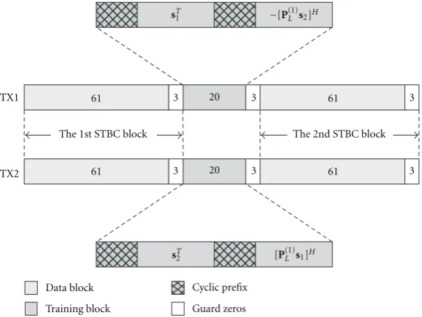
In this section, we provide some simulation results to demonstrate the efficacy of our proposed scheme. In our simulations, we employ a specific block structure for both data and training sequences, which is illustrated inFigure 3, taking the case of NT = 2 as an example. This structure
TX2
TX1 61 3 20 3 61
20 3
61 3 61
3
3
sT1
sT2
−[P(1)L s2]H
[P(1)L s1]H
Guard zeros Data block
Training block
The 2nd STBC block The 1st STBC block
Cyclic prefix
Figure3: Block structure for both data and training sequences.
scheme and various FDE techniques. We assume the channel is frequency selective with channel memory ν = 3, and further assume block fading, that is, the channel fading gains are constant over one ST-coded block including both data and training subblocks, but vary from block to block. For simplicity, we assume no a priori knowledge is available regarding the channel second-order statistics. Hence, only LS method is considered in our simulations. Chu sequences [20], a special case which satisfies the optimal condition given in (32), are chosen to be the training sequences. We use 8-PSK for data transmission without channel coding. At the receiver, channel estimation and equalization are both processed in the frequency domain. As a result, the FFT modules for FDE can be easily reused for the CFR estimation. Several different FDE approaches that are applicable to the structure shown in Figure 3 can be found in [9], and are employed in our simulations.
Figures4(a)and4(b)illustrate the BER performance cor-responding to the frequency-domain MMSE linear equaliza-tion and MMSE decision-feedback equalizaequaliza-tion, respectively, under both CFR estimation and perfect CFR knowledge. When L = 4 (Nb = 14), that is, the minimum length to estimate the CFR, we haveP0 = 16. The performance
penalties due to inaccurate channel estimation, if evaluated at BER = 10−4, are about 2.4 dB for the decision-feedback
equalization and 2.8 dB for the linear equalization. WhenL
extends to 7, or equivalentlyNbextends to 20 as shown in
Figure 3,P0 is accordingly increased to 28. Then, the BER
performance penalties for the decision-feedback equalization and the linear equalization are reduced to 1.1 dB and 1.9 dB, respectively.
Furthermore, we also compare the performance of our approach with the method proposed in [29]. The approach reported in [29] was designed for channel estimation in MIMO systems with SC-FDE. It allows the transmitted sequence to be nulled on certain frequency tones, causing
the transmitted training sequences to be orthogonal in the frequency domain. Essentially, this approach [29] is equivalent to the on-offtype estimation for each channel. To ensure a fair comparison, we apply the reference method [29] to the same structure depicted inFigure 3for the case of NT = 2. Then, both our scheme and the reference
scheme [29] will achieve full rate, that is,R = 1. Since there are 20 symbols in total allocated for the channel parameter estimation in the structure shown in Figure 3, when implementing the approach reported in [29], we allocate 16 for training sequences, and 4 (rather than ν = 3) for the CP. This is because it is required in [29] that the length of training sequences must be evenly divisible by NT. Furthermore, in the simulations, Chu sequences
[20] are also adopted as the training sequences for this benchmark approach, as they as well satisfy the condition of optimality described in [29]. The BER performance of such an algorithm is depicted inFigure 4by dash-dot lines. As illustrated by Figure 4, the system using our proposed scheme performs as well as, if not better than, the system using the approach described in [29]. However, considering the fact that implementation of the method given in [29] requires the transformation from CFR to CIR and then back to CFR (see details in [29]), our approach appears much simpler and straightforward.
CFR estimation withL=4 CFR estimation withL=7
Reference method [29] Ideal CFR knowledge
4 6 8 10 12 14 16 18 20
100
10−1
10−2
10−3
10−4
10−5
BER
22 24
Eb/No(dB)
(a) Linear equalization
4 6 8 10 12 14 16 18 20
100
10−1
10−2
10−3
10−4
10−5
BER
CFR estimation withL=4 CFR estimation withL=7
Reference method [29] Ideal CFR knowledge
Eb/No(dB)
(b) Decision-feedback equalization
Figure4: BER performance with FDE under CFR estimation and perfect CFR knowledge.
4 6 8 10 12 14 16 18 20 22 24
100
10−1
10−2
10−3
10−4
10−5
BER
2TX-1RX with CFR estimation (L=4) 2TX-1RX with ideal CFR knowledge 2TX-2RX with CFR estimation (L=4) 2TX-2RX with ideal CFR knowledge 3TX-1RX with CFR estimation (L=4) 3TX-1RX with ideal CFR knowledge
Eb/No(dB)
Figure5: BER performance comparison for 2TX-1RX, 2TX-2RX, and 3TX-1RX with linear equalization.
performance of the 2TX-1RX case. From these curves, we notice that performance penalties due to inaccurate channel estimation are almost the same for the 1RX and 2TX-2RX cases, but are relatively smaller for the 3TX-1RX case. Furthermore, because of the addition of one more receive antenna, the BER performance of 2TX-2RX is much improved over that of the 2TX-1RX case. However, as shown
in Figure 5, the BER performance of 2TX-2RX is inferior to that of the 3TX-1RX case. This is largely due to the fact that this 3TX-1RX system we consider here is not a full-rate system (i.e.,R=1/2), which is in contrast to those systems employing two transmit antennas and Alamouti-type code.
For the special case of NT = 2, we also conduct
simu-lations to study the behaviors of these adaptive estimation algorithms. For simplicity, Chu sequences [20] are used again in our simulations. We setL=ν+ 1,P0=16, andσn2=0.1. Block fading is still adopted, but the channel fadings are further assumed to be correlated in the time domain. This means the Doppler spread is introduced, and it may affect performance of the adaptive algorithms, as will be confirmed later. The rate of fading in our simulations is determined by
fdT, where fddenotes the maximum Doppler frequency shift andTdenotes the duration of one whole ST-coded block. A larger value of fdT implies faster fading and vice versa. The following simulation results are obtained by setting fdT = 10−4, unless otherwise stated. Figure 6(a) shows a plot of
the squared errore˘F(k)2
versus the number of iterations for a single run or trial of the block-wise LMS and RLS algorithms. Since those algorithms only iterate once for each ST-coded frame, the number of iterations also corresponds to the number of frames. As is shown by Figure 6(a), the learning curves for a single trial of both adaptive algorithms exhibit a noisy form. However, it is clearly seen that the block RLS algorithm converges much faster than the block LMS algorithm. Additionally, we are also interested in the behavior of the squared error deviationvF(k)2
for both algorithms. For the same realization, Figure 6(b) shows the transient behavior of vF(k)2
for both algorithms. As e˘F(k)2
converges,vF(k)2 converges accordingly. But notice that
0 50 100 150 200 0
0.2 0.4 0.6 0.8 1 1.2 1.4 1.6 1.8 2
Number of iterations
Sq
uar
ed
er
ror
Block LMS
Block RLS
(a)˘eF(k)2
0 50 100 150 200
0 1 2 3 4 5 6 7 8 9
Number of iterations
Sq
uar
ed
er
ro
r
Block LMS Block RLS
(b)vF(k)2
Figure6: Transient behavior of squared errore˘F(k)2andvF(k)2of the block-wise LMS and RLS algorithms.fdT=10−4. Block RLS:
λ=0.8; block LMS:μ=0.08.
0 50 100 150 200
0 0.2 0.4 0.6 0.8 1 1.2 1.4 1.6 1.8 2
Number of iterations
M
ean-squar
e
er
ro
r
Block LMS Block RLS
(a) E{e˘F(k)2}
0 50 100 150 200
0 50 100 150 200
0 1 2 3 4 5 6 7 8
Number of iterations
M
ean-squar
e
er
ro
r
0.35 0.4 0.45
Simulated MSE (LS based) Theoretical MSE (LS based) Block RLS
Block LMS
(b) E{vF(k)2} Figure7: Learning curves of the block-wise LMS and RLS algorithms for the mean-square error E{e˘F(k)2
}and E{vF(k)2
}.fdT=10−4.
Block RLS:λ=0.8; block LMS:μ=0.08.
the filter from scratch by simply initializing elements of the channel estimate (i.e., the filter coefficients) all to zeros. This is to demonstrate the convergence performance of these block-wise algorithms. However, in practice, it is certainly possible to speed up the convergence process and reduce the amount of training data. For example, for the first frame, we can obtain the channel estimate by using nonadaptive approach from (49) (i.e.,hot startinitialization). Afterwards, we can apply the adaptive method.
Given the same set of parameters that lead to the results shown in Figure 6, we conduct 100 independent trials and compute the ensemble average. InFigure 7(a), we plot the learning curves of both block-wise algorithms for E{e˘F(k)2}
versus the number of iterations. It is clearly seen that ensemble averaging helps smooth out the effects of gradient noise in the learning curves. For the same set of trials, we also compute the corresponding values of E{vF(k)2}
the purpose of comparison, MSE values obtained from the nonadaptive CFR estimation experiments based on the LS method are also plotted in the same figure, together with the theoretical value. Such a theoretical MSE value can be obtained by plugging these simulation parameters into (33), and we obtain E{EF2} =0
.4. The subplot inFigure 7(b)
indicates a very good match between the simulated values and the theoretical one, which in turn corroborates the correctness of our derivations. Moreover, it is also observed that after the learning curves converge (especially for the block RLS algorithm), the MSE values attained are much smaller than those obtained by the nonadaptive method or the one computed theoretically. This basically demon-strates the performance advantage of using this adaptive approach.
Finally, we provide some simulation results in Figure 8
to demonstrate the error performance of both adaptive esti-mation algorithms at higher Doppler spreads. In particular, we consider three different Doppler spreads: fdT = 10−4, 10−3, and 10−2. And we conduct 100 independent trials for
each case. For simplicity, we leave the step sizes unchanged in our simulations, that is, λ = 0.8 and μ = 0.08; but note that it is desirable to reduce them accordingly as the frequency dispersion or Doppler spread increases. Here, we only study the behavior of E{vF(k)2}
, and for the ease of comparison, we also plot inFigure 8the theoretical MSE value of the nonadaptive LS estimation approach. The results shown inFigure 8indicate that as the Doppler spread increases moderately, for example, from fdT = 10−4 to
fdT=10−3, the estimation accuracy of both algorithms will degrade a little, but not severely. However, further increase in the Doppler spread, for example, from fdT = 10−3 to fdT = 10−2, will lead to a drastic degradation in the estimation accuracy for both algorithms. In fact, in this case, the estimation accuracy of each of these two adaptive algorithms is inferior to that of the nonadaptive estimation approach, indicating that they are unable to track faster channel variations and thus may no longer be usable in practice.
6. Conclusion
In this paper, we presented and studied a training-based CFR estimation scheme for ST-coded MIMO systems with SC-FDE. This scheme is different from the traditional one which obtains the CIR firstly then transfers it to the CFR. In this scheme, CFR estimation is jointly implemented with FDE; thus, estimate of the CFR can be obtained directly and the hardware complexity of the transceiver can also be reduced. To be more specific, training sequences are ST block encoded at the transmitter using the same encoder for data sequences. At the receiver, similar procedures are applied to both data and training sequences, including the CP removal and FFT processing. Then, estimation of the CFR is performed immediately afterwards. Conditioning on different a priori channel knowledge, we further studied the CFR estimation based on two criteria: LS and MMSE. A thorough analysis of the MSE in estimating the CFR
0 50 100 150 200
0 1 2 3 4 5 6 7 8 9
Number of iterations
M
ean-squar
e
er
ro
r
Theoretical MSE (LS based) Block LMS
Block RLS
Block LMS,fdT=1e−2 Block LMS,fdT=1e−3 Block LMS,fdT=1e−4 Block RLS,fdT=1e−2 Block RLS,fdT=1e−3 Block RLS,fdT=1e−4
Figure8: Learning curves of the block-wise LMS and RLS algo-rithms for E{vF(k)2}under different Doppler spreads: fdT =
10−4, 10−3, and 10−2. Block RLS:λ=0.8; block LMS:μ=0.08.
was provided under each criterion. Moreover, imposing a constraint on the transmit power of training sequences, we also investigated the optimal design of training signals. It is shown that under the LS criterion, training sequences having a constant sum magnitude at each frequency tone, such as Chu sequences, will lead to the least MSE. For the MMSE criterion, we have shown that the optimal design of training sequences features a water-filling-type power distribution. Additionally, we demonstrated that adaptive implementation of the CFR is feasible when the number of transmit antennas is equal to 2, which is due to the benign property of Alamouti’s code. However, we feel that the identical property may not be possessed whenNT increases beyond 2 although
it may need further investigation.
Acknowledgments
The work of Z. Shi was supported by the National High-Tech R & D Program of China (863 Program) under Grant No. 2009AA01Z234, China’s National Program on Key Basic Research Project (973 Program) under Grant No. 2007CB310604, and the Important National Science & Technology Specific Projects of China under Grant No. 2009ZX03003-002-01 and No. 2009ZX03003-003-02.