Volume 2006, Article ID 85303, Pages1–11 DOI 10.1155/ASP/2006/85303
Doubly Selective Channel Estimation Using Superimposed
Training and Exponential Bases Models
Jitendra K. Tugnait,1Xiaohong Meng,1, 2and Shuangchi He1
1Department of Electrical and Computer Engineering, Auburn University, Auburn, AL 36849, USA 2Department of Design Verification, MIPS Technologies Inc., Mountain View, CA 94043, USA
Received 1 June 2005; Revised 2 June 2006; Accepted 4 June 2006
Channel estimation for single-input multiple-output (SIMO) frequency-selective time-varying channels is considered using su-perimposed training. The time-varying channel is assumed to be described by a complex exponential basis expansion model (CE-BEM). A periodic (nonrandom) training sequence is arithmetically added (superimposed) at a low power to the information sequence at the transmitter before modulation and transmission. A two-step approach is adopted where in the first step we es-timate the channel using CE-BEM and only the first-order statistics of the data. Using the eses-timated channel from the first step, a Viterbi detector is used to estimate the information sequence. In the second step, a deterministic maximum-likelihood (DML) approach is used to iteratively estimate the SIMO channel and the information sequences sequentially, based on CE-BEM. Three illustrative computer simulation examples are presented including two where a frequency-selective channel is randomly generated with different Doppler spreads via Jakes’ model.
Copyright © 2006 Hindawi Publishing Corporation. All rights reserved.
1. INTRODUCTION
Consider a time-varying SIMO (single-input multiple-out-put) FIR (finite impulse response) linear channel withN out-puts. Let{s(n)}denote a scalar sequence which is input to the SIMO time-varying channel with discrete-time impulse response{h(n;l)}(N-vector channel response at timento a unit input at timen−l). The vector channel may be the result of multiple receive antennas and/or oversampling at the re-ceiver. Then the symbol-rate, channel output vector is given by
x(n) := L
l=0
h(n;l)s(n−l). (1)
In a complex exponential basis expansion representation [4] it is assumed that
h(n;l)= Q
q=1
hq(l)ejωqn, (2)
whereN-column vectorshq(l) (forq=1, 2,. . .,Q) are time-invariant. Equation (2) is a basis expansion ofh(n;l) in the time variablenonto complex exponentials with frequencies {ωq}. The noisy measurements ofx(n) are given by
y(n)=x(n) +v(n). (3)
Equation (2) is the complex-exponential basis expansion model (CE-BEM).
A main objective in communications is to recovers(n) given noisy {y(n)}. In several approaches this requires knowledge of the channel impulse response [11, 19]. In conventional training-based approaches, for time-varying channels, one has to send a training signal frequently and periodically to keep up with the changing channel [7]. This wastes resources. An alternative is to estimate the channel based solely on noisy y(n) exploiting statistical and other properties of {s(n)}[11,19]. This is the blind channel es-timation approach. More recently a superimposed training-based approach has been explored where one takes
CE-BEM representation/approximation of doubly selec-tive channels have been used in [1,2,4–7,15], among oth-ers. Reference [7] deals with time-multiplexed training se-quence design for block transmissions. In this paper we only deal with serial transmissions. In [5], a semiblind approach is considered with time-multiplexed training with serial trans-missions and at least two receive antennas. In this paper our results hold even with one receive antenna. Reference [2] deals with time-varying equalizer design given CE-BEM rep-resentation.
Reference [3] appears to be the first to use (periodic) superimposed training for SISO time-invariant channel es-timation. Periodic training allows for use of the first-order statistics (time-varying mean) of the received signal. Since blind approaches cannot resolve a complex scaling factor am-biguity, they require differential encoding/decoding result-ing in an approximately 3 dB SNR loss. It was noted in [3] that power loss in superimposed training would be typi-cally much less than 3 dB. Furthermore, it was also noted in [3] that identifiability conditions for superimposed training-based methods are much less stringent than that for blind approaches. As noted earlier periodic superimposed train-ing for channel estimation via first-order statistics for SISO systems has been discussed in [17] for both time-invariant and time-varying (CE-BEM based) channels. While in prin-ciple aperiodic superimposed training can also be used, peri-odic training allows for a much simpler algorithm; for in-stance, for CE-BEM channels, relation (13) leads to (19) (see Section 2) which allows for a “decoupled” estimation of the coefficientsdmq (see (10)) from data. In the CE-BEM model the exponential basis functions are orthogonal over the record length. When we use periodic training with ap-propriately selected period in relation to the record length, the “composite” basis functions (ejωmqninSection 2) are still
orthogonal, leading to (13). However, there does not exist any relative advantage or disadvantage between periodic and aperiodic superimposed training when using the iterative ap-proach to joint channel and information sequence estima-tion discussed inSection 3. In the simulations presented in this paper we used an m-sequence (maximal length pseu-dorandom binary sequence) as superimposed training quence. While there exist a large class of periodic training se-quences which are periodically white and/or optimal in some sense (see [9]), some of them do not have a peak-to-average power ratio of one and some of them do not have finite al-phabet, whereas anm-sequence has finite (binary) alphabet and unity peak-to-average power ratio.
As noted earlier, compared to periodically inserted time-multiplexed training (as in [7]), there is no loss in data trans-mission rate in superimposed training. However, there may be an increase in bit-error rate (BER) because of an SNR loss due to power allocated to superimposed training. Our sim-ulation comparisons show that at “low” SNRs we also have a BER advantage (seeExample 3inSection 4). In semi-blind approaches (such as that in [5]), there is periodically inserted time-multiplexed training but one uses the nontraining-based data also to improve the training-nontraining-based results: it uses a combination of training and blind cost functions. While [5]
needs at least two receive antennas, in this paper our results hold even with one receive antenna; besides, in [5] there is still a loss in data transmission rate owing to the presence of time-multiplexed training.
In [17] a first-order statistics-based approach for time-invariant channel estimation using periodic superimposed training has been presented. This approach is further ana-lyzed and enhanced in [18] where a performance analysis has been carried out, and issues such as frame synchroniza-tion and training power allocasynchroniza-tion have been discussed. Both these papers do not deal with time-varying channels; more-over, they do not discuss any iterative approach to joint chan-nel and information sequence estimation even in the context of time-invariant channels.
Objectives and contributions
In this paper, we first present and extend the first-order statistics-based approach of [17] for time-varying (CE-BEM based) channels. Then we extend the first-order statistics-based solution to an iterative approach to joint channel and information sequence estimation, based on CE-BEM, using Viterbi detectors. The first-order statistics-based approach views the information sequence as interference whereas in the iterative joint estimation version it is exploited to en-hance channel estimation and information sequence detec-tion. All results in this paper are developed for an SIMO formulation since everything developed for an SISO system carries over to an SIMO model in a straightforward fashion. However, all our simulations are presented for an SISO sys-tem (for simplicity of presentation).
Notation
Superscripts H, T, and † denote the complex conjugate transpose, the transpose and the Moore-Penrose pseudoin-verse operations, respectively.δ(τ) is the Kronecker delta and IN is theN×N identity matrix. The symbol⊗denotes the Kronecker product. The superscript∗denotes the complex conjugation operation.
1.1. CE-BEM representation
representation
x(n)= L
l=0
h(n;l)s(n−l), (5)
where
h(n;l)= Q
q=1
hq(l)ejωqn, L:=
τd Ts
, (6)
ωq=2π T
q−1 2−
Q 2
, Q:=2fdTTs
+ 1. (7)
This is a scenario where the CE-BEM representation is ap-propriate. The above representation is valid over a duration ofTTsseconds (Tsamples). Equation (1) arises if we follow (5) and consider an SIMO model arising due to multiple an-tennas at the receiver. Although discussed in the context of OFDM, in [12] it is shown that finite-duration observation window effects compromise the accuracy of CE-BEM, that is, CE-BEM is “accurate” only asT→ ∞. One could try to im-prove the CE-BEM efficacy by explicitly incorporating time-domain windowing effects (as in [12]). Such modifications are outside the scope of this paper. We do note that in [8], alternative models (such as polynomial bases models) cou-pled with CE-BEM have been used to improve the modeling results.
2. A FIRST-ORDER STATISTICS-BASED SOLUTION
It is based on CE-BEM. Assume the following:
(H1) the time-varying channel{h(n;l)}satisfies (2) where the frequencies ωq (q = 1, 2,. . .,Q) are distinct and known withωq∈[0, 2π). AlsoN≥1. For someq(1≤ q≤Q), we haveωq=0;
(H2) the information sequence{b(n)}is zero-mean, white withE{|b(n)|2} =1;
(H3) the measurement noise {v(n)} is nonzero-mean (E{v(n)} =m), white, uncorrelated with{b(n)}, with E{[v(n+τ)−m][v(n)−m]H} =σ2
vINδ(τ). The mean vectormmay be unknown;
(H4) the superimposed training sequencec(n)=c(n+mP) for allm,nis a nonrandom periodic sequence with pe-riodP.
For model (7), we haveq=(Q+ 1)/2. Negative values ofωq’s in (7) are to be interpreted as positive values after a modulo 2πoperation, that is, in (7), for 1≤q < q, we also haveωq= (2π/T)(q−1/2−Q/2 +T).
In this section, we will exploit the first-order statistics (i.e.,E{y(n)}) of the received signal. (A consequence of us-ing the first-order statistics is that the knowledge of the noise varianceσ2
vin (H3) is not used here.) By (H4), we have
c(n)= P−1
m=0
cmejαmn ∀n, (8)
where
cm:= 1 P
P−1 n=0
c(n)e−jαmn, α
m:=2πm
P . (9)
The coefficientscm are known at the receiver since{c(n)}is known. By (1)–(3), (8)-(9), and (H3), we have
E y(n)= Q
q=1 P−1 m=0
L
l=0
cmhq(l)e−jαml
=:dmq
ej(ωq+αm)n+m.
(10) Suppose that we pickPto be such that (ωq+αm)’s are all distinct for any choice ofmandq. For instance, suppose that the data record lengthTsamples (see alsoSection 1.1) andP are such thatT=KPfor some integerK >0. In such a case, we have
ωmq :=ωq+αm
(11) = ⎧ ⎪ ⎪ ⎪ ⎨ ⎪ ⎪ ⎪ ⎩ 2π T
q−1 2−
Q 2 +Km
mod(2π) ifQ≥q≥Q+ 1 2 , 2π
T
q−1 2−
Q
2+T+Km
mod(2π) if 1≤q < Q+ 1 2 .
(12) IfP andK are such thatK ≥ Q, then it follows from (12) thatωm1q1 =ωm2q2 ifq1=q2orm1=m2. Henceforth, it is assumed that the above conditions hold true. Then we have
T−1T
−1
n=0
ej(2π/T)(q+Km)n=δ(q)δ(m). (13)
Note thatωmq = 0 only when m = 0 andq = q. We rewrite (10) as
E y(n)= Q
q=1 P−1
m=0(q,m)=(q,0)
dmqejωmqn+
d0q+m
. (14)
Given the observation sequencey(n), 0 ≤ n ≤ T−1, our approach to estimatinghq(l)’s using the first-order statistics of the data is to first estimate dmq’s for 0 ≤ m ≤ P−1, 1≤q≤Q((q,m)=(q, 0)), and then estimatehq(l)’s from the estimateddmq’s. By (14),dmqis the coefficient of the ex-ponentialejωmqnfor (q,m)= (q, 0), whereasd
0q+m is the coefficient ofejω0qn=1. Since the dc offsetmis not
necessar-ily known, we will not seek the coefficient ofejω0qnin (14). By
(1)–(3) and (14), we have
y(n)= Q
q=1 P−1 m=0
dmq+mδ(q−q)δ(m)
ejωmqn+e(n),
(15) wheree(n) is a zero-mean random sequence. Define the cost function
J= T−1
n=0
e(n)2
Choosedmq’s (q =1, 2,. . .,Q; m=0, 1,. . .,P−1, (q,m)= (q, 0)) to minimizeJ. For optimization, we must have
∂J ∂d∗
mq
dmq=dmq
∀q,m
=0, (17)
where the partial derivative in (17) for givenmandq is a column vector of dimensionN(the derivatives are compo-nentwise). (17) leads to
T−1 n=0
e(n)e−jωmqn
dmq=dmq
∀q,m
=0. (18)
Using (13), (15), and (18), it follows that (for (q,m)=(q, 0))
dmq= 1 T
T−1 n=0
y(n)e−jωmqn. (19)
It follow from (14) and (19) that
E dmq
=dmq, (q,m)=(q, 0). (20)
Now we establish that givendmqfor 1≤q≤Qand 0≤ m ≤ P−1 but excludingωq+αm =0, we can (uniquely) estimatehq(l)’s ifP≥L+ 2 andcm=0 for allm=0. Define
V:=
⎡ ⎢ ⎢ ⎢ ⎢ ⎢ ⎣
1 e−jα1 · · · e−jα1L 1 e−jα2 · · · e−jα2L ..
. ... ... ... 1 e−jαP−1 · · · e−jαP−1L
⎤ ⎥ ⎥ ⎥ ⎥ ⎥ ⎦
(P−1)×(L+1)
, (21)
Dm:=
dTm1,dTm2,. . .,dTmQT, (22) Hl:=
hT
1(l),hT2(l),. . .,hTQ(l)
T
, (23)
H :="HH0 HH1 · · · HHL
#H
, (24)
D1:=
"
DH1 DH2 · · · DHP−1
#H
, (25)
C1:=
diag c1,c2,. . .,cP−1
V
=:V
⊗INQ. (26)
Omitting the termm=0 and using the definition ofdmqfrom (10), it follows that
C1H =D1. (27)
Notice that we have omitted all pairs (m,q)=(0,q) (q= q) from (27). In order to include these omitted terms, we further define an [N(Q−1)]-column vector
D0:=
dT01,dT02,. . .,dT0(q−1)dT0(q+1),. . .,dT0Q
T
, (28)
an [N(Q−1)]×[NQ] matrix
A:=
IN(q−1) 0 0 0 0 IN(Q−q)
, (29)
and an [N(Q−1)]×[NQ(L+ 1)] matrix
C2:=
"
c0A c0A · · · c0A#. (30)
Then it follows from (10) and (28)–(30) that
C2H =D0. (31)
In order to concatenate (27) and (31), we define
C:=
C2
C1
, D:=
D0
D1
, (32)
which lead to
CH =D. (33)
Equation (33) utilizes all pairs (m,q) except (0,q).
In (21)Vis a Vandermonde matrix with a rank ofL+ 1 if P−1≥L+1 andαm’s are distinct [14, page 274]. Sincecm=0 for allm, by [14, Result R4, page 257], rank(V)=rank(V)= L+ 1. Finally, by [10, Property K6, page 431], rank(C1) = rank(V)×rank(INQ) = NQ(L+ 1). Therefore, we can de-termine hq(l)’s uniquely from (27). Augmenting (27) with additional equations to obtain (33) keeps the earlier conclu-sions unchanged, that is, rank(C)=rank(C1)=NQ(L+ 1). Thus, ifP≥L+ 2 andcm=0 for allm=0, (33) has a unique solution forH(i.e.,hq(l)’s).
DefineDm as in (22) or (28) with dmq’s replaced with
dmq’s. Similarly, define$Das in (25) and (32) withDm’s re-placed withDm’s. Then from (33) we have the channel esti-mate
$
H =CHC−1CH$D. (34)
By (20) and (33), it follows that
E{H$} =H. (35)
We summarize our method in the following lemma. Lemma 1. Under (H1)–(H4), the channel estimator(34) sat-isfies (35) under the following (additional) sufficient condi-tions: the periodic training sequence is such that cm = 0for allm=0,P≥L+ 2, andPandT are such thatT =KPfor integerK≥Q.
Remark 1. A more logical approach would have been to se-lecthq(l)’s andmjointly to minimize the costJin (16). The resulting solution is more complicated and it couples esti-mates ofhq(l)’s andm. Since we do not used0q, we are dis-carding any information abouthq(l) therein.
Remark 3. The cost (16) is not novel; it also occurs in [1,15] in the context of time-multiplexed training for doubly se-lective channels. However, unlike these papers, as noted in Remark 1 we do not directly estimate hq(l)’s and m (there is no m in these papers); rather, we first estimate dmq’s which are motivated through the time-varying mean E{y(n)}, hence, the term first-order statistics. This aspect is missing from [1,15], and in this paper it is motivated by the time-invariant results of [9,16,21] (among others). Choice of periodic superimposed training is also motivated by the results of [9,16,21].
3. DETERMINISTIC MAXIMUM-LIKELIHOOD (DML) APPROACH
The first-order statistics-based approach ofSection 2views the information sequence as interference. Since the training and information sequences of a given user pass through an identical channel, this fact can be exploited to enhance the channel estimation performance via an iterative approach. We now consider joint channel and information sequence estimation via an iterative DML (or conditional ML) ap-proach assuming that the noisev(n) is complex Gaussian. We have guaranteed convergence to a local maximum. Further-more, if we initialize with our superimposed training-based solution, one is guaranteed the global extremum (minimum error probability sequence estimator) if the superimposed training-based solution is “good.”
Suppose that we have collectedT−Lsamples of the ob-servations. Form the vector
Y=yT(T−1),yT(T−2),. . .,yT(L)T (36)
and similarly define
s:=s(T−1),s(T−2),. . .,s(0)T. (37)
Furthermore, let
%
v(n) :=v(n)−m. (38)
Using (1)–(3) we then have the following linear model:
Y =T(s)H+
⎡ ⎢ ⎢ ⎣ %
v(T−1) .. .
%
v(L)
⎤ ⎥ ⎥ ⎦
=:V% + ⎡ ⎢ ⎢ ⎣ m .. . m ⎤ ⎥ ⎥ ⎦
=:M
, (39)
whereV =V% +Mis a column-vector consisting of samples of noise{v(n)}in a manner similar to (36),His defined in (24),T(s) is a block Hankel matrix given by
T(s) :=
⎡ ⎢ ⎢ ⎢ ⎢ ⎢ ⎣
s(T−1)ΣT−1 · · · s(T−L−1)ΣT−1 s(T−2)ΣT−2 · · · s(T−L−2)ΣT−2
..
. ... ...
s(L)ΣL · · · s(0)ΣL
⎤ ⎥ ⎥ ⎥ ⎥ ⎥ ⎦, (40)
a block Hankel matrix has identical block entries on its block antidiagonals, and
Σn:=
"
ejω1nI
N ejω2nIN · · · ejωQnIN
#
. (41)
Also using (1)–(3), an alternative linear model forYis given by
Y =F(H)s+V%+M, (42) where
F(H) :=
⎡ ⎢ ⎢ ⎣
h(T−1; 0) · · · h(T−1;L)
. .. . ..
h(L; 0) · · · h(L;L)
⎤ ⎥ ⎥ ⎦
(43) is a “filtering matrix.”
Consider (1), (3), and (39). Under the assumption of temporally white complex Gaussian measurement noise, consider the joint estimators
$H,s,m=arg&min
H,s,m
Y−T(s)H−M2'
, (44)
wheresis the estimate ofs. In the above we have followed a DML approach assuming no statistical model for the input sequences{s(n)}. Using (39) and (42), we have a separable nonlinear least-squares problem that can be solved sequen-tially as (joint optimization with respect toH,mcan be fur-ther “separated”)
$H,s,m=arg min
s
&
min
H,m
Y−T(s)H−M2'
=arg min
H,m
&
min
s Y−F(H)s−M
2' .
(45)
The finite alphabet properties of the information sequences can also be incorporated into the DML methods. These al-gorithms, first proposed by Seshadri [13] for time-invariant SISO systems, iterate between estimates of the channel and the input sequences. At iterationk, with an initial guess of the channelH(k)and the meanm(k), the algorithm estimates the input sequences(k)and the channelH(k+1)and meanm(k+1) for the next iteration by
s(k)=arg min
s∈S Y−F
H(k)s−M(k)2, (46)
H(k+1)=arg min
H Y−T
s(k)H−M(k)2, (47) m(k+1)=arg min
m Y−T
s(k)H(k+1)−M2
, (48)
We now summarize our DML approach in the following steps.
(1) (a) Use (34) to estimate the channel using the first-order (cyclostationary) statistics of the obser-vations. Denote the channel estimates by H$(1) andh(1)q (l). In this method{c(n)}is known and {b(n)}is regarded as interference.
(b) Estimate the meanm(1)as follows. Define (recall (1)–(3))
m(1):=
1 T
T−1
n=0
y(n)− L
l=0
h(1)(n;l)c(n−l)
,
h(1)(n;l) := Q
q=1
h(1)q (l)ejωqn.
(49)
(c) Design a Viterbi sequence detector to estimate {s(n)} as {%s(n)} using the estimated channel
$
H(1), meanm(1)and cost (46) withk=1. (Note that knowledge of{c(n)}is used ins(n)=b(n) + c(n), therefore, we are in essence estimatingb(n) in the Viterbi detector.)
(2) (a) Substitute%s(n) for s(n) in (1) and use the cor-responding formulation in (39) to estimate the channelHas
$
H(2)=T†(%s)Y−M$(1)
. (50)
Defineh(2)(n;l) usingh(2)
q (l) in a manner simi-lar toh(1)(n;l). Then the meanmis estimated as
m(2)given by
m(2)= 1 T−L
T−1
n=L
y(n)− L
l=0
s(1)(n−l)h(2)(n;l)
. (51)
(b) Design a Viterbi sequence detector using the esti-mated channel H$(2), mean m(2), and cost (46) withk=2, as in step (1)(c).
(3) Step (2) provides one iteration of (46)-(47). Repeat a few times till any (relative) improvement in chan-nel estimation over previous iteration is below a pre-specified threshold.
4. SIMULATION EXAMPLES
We now present several computer simulation examples in support of our proposed approach.Example 1uses an exact CE-BEM representation to generate data whereas Examples 2and3use a 3-tap Jakes’ channel to generate data. In all ex-amples CE-BEMs are used to process the observations; there-fore, in Examples2and3we have approximate modeling. Example 1. In this example we pick an arbitrary value ofQ independent ofT. In (2) takeN=1,Q=2, and
ω1=0, ω2=2π
50. (52)
We consider a randomly generated channel in each Monte Carlo run with random channel lengthL∈ {0, 1, 2}picked with equal probabilities and random channel coefficients hq(l), 0 ≤ l ≤ L, taken to be mutually independent com-plex random variables with independent real and imag-inary parts, each uniformly distributed over the interval [−1, 1]. Normalized mean-square error (MSE) in estimat-ing the channel coefficientshq(l), averaged over 100 Monte Carlo runs, was taken as the performance measure for chan-nel identification. It is defined as (before Monte Carlo aver-aging)
NCMSE1:=
& (Q q=1
(2
m=0hq(m)−hq(m) 2'
(Q
q=1
(2
m=0hq(m)2
(53)
The training sequence was taken to be anm-sequence (maxi-mal length pseudorandom binary sequence) of length 7 (=P)
c(n)6n=0= {1,−1,−1, 1, 1, 1,−1}. (54) The input information sequence{b(n)}is i.i.d. equiprobable 4-QAM. As in [9,16], define a power loss factor
α= σb2 σ2
b+σc2
(55)
and power loss−10 log(α) dB, as a measure of the informa-tion data power loss due to the inclusion of the training se-quence. Here
σb2:=E
&
b(n)2', σ2 c :=
1 P
P−1 n=0
c(n)2
. (56)
The training sequence was scaled to achieve a desired power loss. Complex white zero-mean Gaussian noise was added to the received signal and scaled to achieve a desired signal-to-noise (SNR) ratio at the receiver (relative to the contribution of{s(n)}).
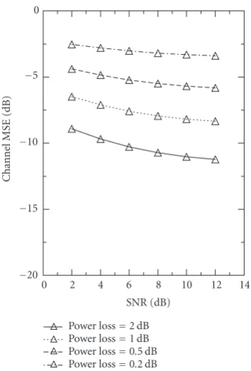
Our proposed method usingL=Lu=4 (channel length overfit) in (34) was applied for varying power losses due to the superimposed training sequence.Figure 1shows the sim-ulation results. It is seen that as α decreases (i.e., training power increases relative to the information sequence power), one gets better results. Moreover, the proposed method works with overfitting. Finally, adding nonzero mean (dc off -set) to additive noise yielded essentially identical results (dif-ferences do not show on the plotted curves).
Example 2. Consider (1) withN =1 andL=2. We simu-late a random time-and frequency-selective Rayleigh fading channel following [20]. For differentl’s,h(n;l)’s are mutually independent and for a givenl, we follow the modified Jakes’ model [20] to generateh(n;l):
h(n;l)=X(t)|t=nTs, (57)
0 2 4 6 8 10 12 14 20
15 10 5 0
SNR (dB)
Channel
M
SE
(dB)
Power loss=2 dB Power loss=1 dB Power loss=0.5 dB Power loss=0.2 dB
Figure1:Example 1. Normalized channel MSE (53) based onT=
140 symbols per run, 100 Monte Carlo runs, QPSK signal,P =7. Power loss= −10 log(α) dB whereαis as in (55).
over [0, 2π),Tsdenotes the symbol interval, fd denotes the (max.) Doppler spread, andM=25. For a fixedl, (57) gen-erates a random process{h(n;l)}n whose power spectrum approximates the Jakes’ spectrum asM ↑ ∞. We consider a system with carrier frequency of 2 GHz, data rate of 40 kB (kB=kilo-Bauds), therefore,Ts=25×10−6seconds, and a varying Doppler spread fdin the range 0 Hz to 200 Hz (cor-responding to a maximum mobile velocity in the range 0 to 108 km/hr). We picked a data record length of 400 symbols (time duration of 10 msec). For a given Doppler spread, we pickQas inSection 1.1(T=400,L=2 in (7)). For the cho-sen parameters it varies within the values{1, 3, 5}. We em-phasize that the CE-BEM was used only for processing at the receiver; the data were generated using (57).
We take all sequences (information and training) to be binary. For superimposed training, we take a periodic (scaled) binary sequence of periodP =7 with the training-to-information sequence power ratio (TIR) of 0.3 where
TIR=σc2 σ2 b
=α−1−1 (58)
andσ2
b andσc2denote the average power in the information sequence{b(n)}and training sequence{c(n)}, respectively. Complex white zero-mean Gaussian noise was added to the received signal and scaled to achieve a target bit SNR at the receiver (relative to the contribution of{s(n)}).
For comparison, we consider conventional time-multi-plexed training assuming time-invariant channels, as well as
CE-BEM-based periodically placed time-multiplexed train-ing with and without zero-paddtrain-ing, followtrain-ing [7]. In the for-mer, the block of data of length 400 symbols was split into two nonoverlapping blocks of 200 symbols each. Each sub-block had a training sequence length of 46 symbols in the middle of the data subblock with 154 symbols for informa-tion; this leads to a training-to-information sequence power ratio (over the block length) of approximately 0.3. Assuming synchronization, time-invariant channels were estimated us-ing conventional trainus-ing and used for information detection via a Viterbi algorithm; this was done for each subblock. In the CE-BEM set-up, following [7], we took a training block of length 2L+ 1=5 and a data block of length 17 bits lead-ing to a frame of length 22 bits. This frame was repeated over the entire record length (22×18). Thus, we have a training-to-information bit ratio of approximately 0.3. Two versions of training sequences were considered. In one of them zero-padding was used with a random bit in the middle of the training block, as in [7]: this leads to a peak-to-average power ratio (PAR) of 5. In the other version we had a random binary sequence of length 5 in each training block, leading to a PAR of 1 (an ideal choice). Assuming synchronization, CE-BEM channel was estimated using conventional training and used for information detection via a Viterbi algorithm. We also considered another variation of zero-padded training with a training block of length 2L+ 1=5 but a data block of length 50 bits leading to a training-to-information bit ratio of 0.1. Thus the proposed superimposed training scheme results in a data transmission rate that is 30% higher than the data trans-mission rate in all of the time-multiplexed training schemes considered in this example, except for the last scheme com-pared to which the data transmission rate is 10% higher.
Figure 2 shows the BER (bit error rate) based on 500 Monte Carlo runs for conventional training based on time-invariant (TI) modeling, the CE-BEM-based periodically placed time-multiplexed training for PAR = 5 and PAR = 1, the first-order statistics and superimposed training-based method and the proposed DML approach with two itera-tions, under varying Doppler spreads fd and a bit SNR of 25 dB. It is seen that as Doppler spread fdincreases beyond about 60 Hz (normalized DopplerTsfdof 0.0015), superim-posed training approach ofSection 2(step (1)) outperforms the conventional (midamble) training with time-invariant channel approximation, without decreasing the data trans-mission rate. Furthermore, the proposed DML enhancement can lead to a significant improvement with just one iteration. On the other hand, the CE-BEM-based periodically placed time-multiplexed training approach of [7] significantly out-performs the superimposed training-based approaches, but at the cost of a reduction in the data transmission rate. Figure 3shows the normalized channel mean-square error (NCMSE), defined (before averaging over runs) as
NCMSE=
(T
n=1
(2
l=0h(n;l)−h(n;l) 2
(T
n=1
(2
l=0h(n;l)
0 20 40 60 80 100 120 140 160 180 200 10 6
10 5 10 4 10 3 10 2 10 1 100
fd(Doppler spread, Hz)
BER
Conv. training, TI model: 46 + 46 bits in the middle Superimposed training: step 1, TIR=0.3 Superimposed training: 1st iteration, TIR=0.3 Superimposed training: 2nd iteration, TIR=0.3 Conv. training, TV model, PAR=5, TIR=0.1 Conv. training, TV model, PAR=5, TIR=0.3 Conv. training, TV model, PAR=1, TIR=0.3 SISO system; data 400
500; SNR=25 dB; Viterbi algorithm
Figure2:Example 2. BER: circle: estimate channel using superimposed training (training-to-information symbol power ratio TIR=0.3) and then design a Viterbi detector; square: first iteration specified by step (2) (Section 3); up-triangle: second iteration specified by step (2) (Section 3); dot-dashed: estimate channel using conventional time-multiplexed training of length 46 bits in the middle of a subblock of length 200 bits and then design a Viterbi detector; cross: CE-BEM-based periodically placed time-multiplexed training with zero padding [7], TIR=0.3; star: CE-BEM-based periodically placed time-multiplexed training without zero padding, TIR=0.3; down-triangle: CE-BEM-based periodically placed time-multiplexed training with zero-padding [7], TIR=0.1. SNR=25 dB. Record length=400 bits. Results are based on 500 Monte Carlo runs.
0 20 40 60 80 100 120 140 160 180 200 50
45 40 35 30 25 20 15 10 5 0
fd(Doppler spread, Hz)
NCMSE
(dB)
Superimposed training: step 1, TIR=0.3 Superimposed training: 1st iteration, TIR=0.3 Superimposed training: 2nd iteration, TIR=0.3 Conv. training, TV model, PAR=5, TIR=0.1 Conv. training, TV model, PAR=5, TIR=0.3 Conv. training, TV model, PAR=1, TIR=0.3 SISO system; data 400500; SNR=25 dB; Viterbi algorithm
0 5 10 15 20 25 30 10 3
10 2 10 1 100
SNR (dB)
BER
Superimposed training: 2nd iteration, TIR=0.3 Conv. training, TV model, PAR=5, TIR=0.1 Conv. training, TV model, PAR=5, TIR=0.3 SISO system; data 400500;
fd=120 Hz; Viterbi algorithm
Figure4:Example 3. BER for varying SNR with Doppler spreadfd=120 Hz: up-triangle: superimposed training, second iteration specified by step (2) (Section 3), TIR=0.3; cross: CE-BEM-based periodically placed time-multiplexed training with zero padding [7], TIR=0.3; down-triangle: CE-BEM-based periodically placed time-multiplexed training with zero padding [7], TIR=0.1. After estimating the channel, we design a Viterbi detector using the estimated channel. Record length=400 bits. Results are based on 500 Monte Carlo runs.
0 5 10 15 20 25 30
16 14 12 10 8 6 4 2 0 2 4
SNR (dB)
NCMSE
(dB)
Superimposed training: 2nd iteration, TIR=0.3 Conv. training, TV model, PAR=5, TIR=0.1 Conv. training, TV model, PAR=5, TIR=0.3 SISO system; data 400500;
fd=120 Hz; Viterbi algorithm
Figure5:Example 3. As inFigure 4except that corresponding NCMSE (normalized channel mean-suare error) (59) is shown.
Example 3. To further compare the relative advantages and disadvantages of CE-BEM-based superimposed training and periodically placed time-multiplexed training, we now repeat Example 2but with varying SNR; the other details remain unchanged. Figures4and5show the simulation results for a Doppler spread of 120 Hz (normalized Doppler spread of 0.003 for bit duration of Ts = 25μs) where we compare the results of the second iteration of the proposed DML ap-proach based on superimposed training with that of peri-odically placed time-multiplexed training. There is an error floor with increasing SNR which is attributable to modeling
errors in approximating the Jakes’ model with CE-BEM. It is seen fromFigure 4that our proposed approach outperforms (better BER) the CE-BEM-based periodically placed time-multiplexed training approach of [7] for SNRs at or below 10 dB, and underperforms for SNRs at or above 20 dB. There is also the data transmission rate advantage at all SNRs.
5. CONCLUSIONS
based) channel estimation using superimposed training. Then we extended the first-order statistics-based solution to an iterative approach to joint channel and information sequence estimation, based on CE-BEM, using Viterbi de-tectors. The first-order statistics-based approach views the information sequence as interference whereas in the itera-tive joint estimation version it is exploited to enhance chan-nel estimation and information sequence detection. The re-sults were illustrated via several simulation examples some of them involving time-and frequency-selective Rayleigh fading where we compared the proposed approaches to some of the existing approaches. Compared to the CE-BEM-based peri-odically placed time-multiplexed training approach of [7], one achieves a lower BER for SNRs at or below 10 dB, and higher BER for SNRs at or above 20 dB. There is also the data transmission rate advantage at all SNRs. Further work is needed to compare the relative advantages and disadvan-tages of CE-BEM-based superimposed training and periodi-cally placed time-multiplexed training.
ACKNOWLEDGMENTS
This work was supported by the US Army Research Office under Grant DAAD19-01-1-0539 and by NSF under Grant ECS-0424145. Preliminary versions of the paper were pre-sented in parts at the 2003 and the 2004 IEEE International Conferences on Acoustics, Speech, Signal Processing, Hong Kong, April 2003 and Montreal, May 2004, respectively.
REFERENCES
[1] M.-A. R. Baissas and A. M. Sayeed, “Pilot-based estimation of time-varying multipath channels for coherent CDMA re-ceivers,”IEEE Transactions on Signal Processing, vol. 50, no. 8, pp. 2037–2049, 2002.
[2] I. Barhumi, G. Leus, and M. Moonen, “Time-varying FIR equalization for doubly selective channels,”IEEE Transactions on Wireless Communications, vol. 4, no. 1, pp. 202–214, 2005. [3] B. Farhang-Boroujeny, “Pilot-based channel identification:
proposal for semi-blind identification of communication channels,”Electronics Letters, vol. 31, no. 13, pp. 1044–1046, 1995.
[4] G. B. Giannakis and C. Tepedelenlioglu, “Basis expansion models and diversity techniques for blind identification and equalization of time-varying channels,” Proceedings of the IEEE, vol. 86, no. 10, pp. 1969–1986, 1998.
[5] G. Leus, “Semi-blind channel estimation for rapidly time-varying channels,” in Proceedings of the IEEE International Conference on Acoustics, Speech, and Signal Processing (ICASSP ’05), vol. 3, pp. 773–776, Philadelphia, Pa, USA, March 2005. [6] X. Ma and G. B. Giannakis, “Maximum-diversity
transmis-sions over doubly selective wireless channels,”IEEE Transac-tions on Information Theory, vol. 49, no. 7, pp. 1832–1840, 2003.
[7] X. Ma, G. B. Giannakis, and S. Ohno, “Optimal training for block transmissions over doubly selective wireless fad-ing channels,”IEEE Transactions on Signal Processing, vol. 51, no. 5, pp. 1351–1366, 2003.
[8] X. Meng and J. K. Tugnait, “Superimposed training-based doubly-selective channel estimation using exponential and polynomial bases models,” inProceedings of the 38th Annual
Conference on Information Sciences & Systems (CISS ’04), Princeton University, Princeton, NJ, USA, March 2004. [9] A. G. Orozco-Lugo, M. M. Lara, and D. C. McLernon,
“Chan-nel estimation using implicit training,”IEEE Transactions on Signal Processing, vol. 52, no. 1, pp. 240–254, 2004.
[10] B. Porat,Digital Processing of Random Signals, Prentice-Hall, Englewood Cliffs, NJ, USA, 1994.
[11] J. G. Proakis, Digital Communications, McGraw-Hill, New York, NY, USA, 4th edition, 2001.
[12] P. Schniter, “Low-complexity equalization of OFDM in dou-bly selective channels,”IEEE Transactions on Signal Processing, vol. 52, no. 4, pp. 1002–1011, 2004.
[13] N. Seshadri, “Joint data and channel estimation using blind trellis search techniques,”IEEE Transactions on Communica-tions, vol. 42, no. 2–4, part 2, pp. 1000–1011, 1994.
[14] P. Stoica and R. L. Moses,Introduction to Spectral Analysis, Prentice-Hall, Englewood Cliffs, NJ, USA, 1997.
[15] M. K. Tsatsanis and G. B. Giannakis, “Modeling and equaliza-tion of rapidly fading channels,”International Journal of Adap-tive Control & Signal Processing, vol. 10, no. 2-3, pp. 159–176, 1996.
[16] J. K. Tugnait and W. Luo, “On channel estimation using super-imposed training and first-order statistics,”IEEE Communica-tions Letters, vol. 7, no. 9, pp. 413–415, 2003.
[17] , “On channel estimation using superimposed train-ing and first-order statistics,” inProceedings of the IEEE Inter-national Conference on Acoustics, Speech and Signal Processing (ICASSP ’03), vol. 4, pp. 624–627, Hong Kong, April 2003. [18] J. K. Tugnait and X. Meng, “On superimposed training for
channel estimation: performance analysis, training power al-location, and frame synchronization,”IEEE Transactions on Signal Processing, vol. 54, no. 2, pp. 752–765, 2006.
[19] J. K. Tugnait, L. Tong, and Z. Ding, “Single-user channel es-timation and equalization,”IEEE Signal Processing Magazine, vol. 17, no. 3, pp. 16–28, 2000.
[20] Y. R. Zheng and C. Xiao, “Simulation models with correct sta-tistical properties for Rayleigh fading channels,”IEEE Transac-tions on CommunicaTransac-tions, vol. 51, no. 6, pp. 920–928, 2003. [21] G. T. Zhou, M. Viberg, and T. McKelvey, “A first-order
statis-tical method for channel estimation,”IEEE Signal Processing Letters, vol. 10, no. 3, pp. 57–60, 2003.
Jitendra K. Tugnaitreceived the B.S. degree with honors in electronics and electrical communication engineering from the Pun-jab Engineering College, Chandigarh, India, in 1971, the M.S. and the E.E. degrees from Syracuse University, Syracuse, NY, and the Ph.D. degree from the University of Illinois at Urbana-Champaign, in 1973, 1974, and 1978, respectively, all in electrical engineer-ing. From 1978 to 1982, he was an Assistant
on Signal Processing. He is currently an Editor of the IEEE Transac-tions on Wireless CommunicaTransac-tions and an Associate Editor of IEEE Signal Processing Letters. He was elected Fellow of IEEE in 1994.
Xiaohong Meng was born in Luoyang, He’nan Province, China, on June 12, 1973. She received her B.E. degree in 1995 in elec-trical engineering from Beijing University of Posts and Telecommunications. From 1995 to 1999, she held the position of Instruc-tor at He’nan Posts and Telecommunica-tions School. From September 1995 to June 2001, she studied as a graduate student at Beijing University of Posts and
Telecommu-nications. From January 2002 to May 2005, she was a Research Assistant in Electrical and Computer Engineering Department of Auburn University. She received her Ph.D. degree in electrical en-gineering in May 2005 and her M.S. degree in mathematics in May 2006 from Auburn University. She joined MIPS Technologies, Mountain View, Calif, in March 2006. Her current research inter-ests include digital signal processing, statistical signal processing, wireless communications, and semiblind equalization.
Shuangchi He received the B.E. and M.S. degrees in electronic engineering from Ts-inghua University, Beijing, China, in 2000 and 2003, respectively. He is currently working towards his Ph.D. degree in electri-cal engineering at Auburn University. Since 2003, he has been a Graduate Research As-sistant at the Department of Electrical and Computer Engineering, Auburn University. His research interests include channel