Probabilistic Model Checking
Tim Kemna
Master’s Thesis in Computer Science
August 2006
University of Twente Graduation committee: Faculty of EEMCS prof. dr. ir. J.-P. Katoen Formal Methods and Tools dr. D. N. Jansen
Working on my Master’s thesis was one of the most challenging parts of my studies Computer Science at the University of Twente. I learnt a lot about an interesting research area which was relatively new to me when I started this assignment: probabilistic model checking. Also, I have been given the opportunity to look inside a model checker and to implement an extension for it.
Finally, I would like to thank Joost-Pieter Katoen and David Jansen for their supervision and support. Last, but not least, I would like to thank Ivan Zapreev for answering all my questions concerning MRMC.
Tim Kemna,
1 Introduction 13
2 Preliminaries 15
2.1 Discrete-time Markov chains . . . 15
2.2 Continuous-time Markov chains . . . 16
2.3 Probabilistic Computation Tree Logic . . . 17
2.3.1 Syntax and semantics . . . 18
2.3.2 Model checking . . . 19
2.4 Continuous Stochastic Logic . . . 20
2.4.1 Syntax and semantics . . . 21
2.4.2 Model checking . . . 21
2.5 Bisimulation equivalence . . . 23
2.5.1 The discrete-time setting . . . 23
2.5.2 The continuous-time setting . . . 24
2.6 Lumping algorithm . . . 24
3 Implementation of the lumping algorithm 29 3.1 The Markov Reward Model Checker . . . 29
3.2 Implementing the lumping algorithm . . . 30
3.2.1 Data structures . . . 30
3.2.2 The initial partition . . . 32
3.2.3 Procedure LUMP . . . 33
4 Bisimulation minimisation and PCTL model checking 35
4.1 Introduction . . . 35
4.2 PCTL properties . . . 36
4.3 Case studies . . . 37
4.3.1 Synchronous Leader Election Protocol . . . 37
4.3.2 Randomised Self-stabilisation . . . 39
4.3.3 Crowds Protocol . . . 40
4.3.4 Randomised Mutual Exclusion . . . 43
4.4 Conclusion . . . 44
5 Formula-dependent lumping for PCTL model checking 47 5.1 Introduction . . . 47
5.2 Bisimulation equivalence . . . 47
5.3 PCTL properties . . . 50
5.4 Case studies . . . 51
5.4.1 Randomised Mutual Exclusion . . . 52
5.4.2 Workstation Cluster . . . 52
5.4.3 Cyclic Server Polling System . . . 54
5.5 Conclusion . . . 56
6 Bisimulation minimisation and CSL model checking 57 6.1 Introduction . . . 57
6.2 CSL properties . . . 57
6.3 Symmetry reduction . . . 58
6.4 Case studies . . . 59
6.4.1 Workstation Cluster . . . 59
6.4.2 Cyclic Server Polling System . . . 62
6.4.3 Tandem Queueing Network . . . 63
6.4.4 Simple Peer-To-Peer Protocol . . . 64
7 Formula-dependent lumping for CSL model checking 67
7.1 Introduction . . . 67
7.2 Bisimulation equivalence . . . 67
7.3 CSL properties . . . 68
7.4 Case studies . . . 69
7.4.1 Workstation Cluster . . . 69
7.4.2 Cyclic Server Polling System . . . 71
7.4.3 Tandem Queueing Network . . . 72
7.5 Conclusion . . . 73
8 Conclusion 75
Introduction
Model checking [9] is a technique for verifying software or hardware systems in an automated way, such as real-time embedded or safety-critical systems. Using a formal language, we can define a model which describes the system requirements or the design of the system. A model checking tool verifies if the model satisfies a formal specification, called a property or formula. This specification is often expressed in a temporal logic, such as Computation Tree Logic (CTL) [8]. In other words, model checking is a technique to establish the correctness of the system.
Probabilistic model checking is a verification technique for probabilistic systems. In these systems, there is a certain probability associated with events. The probabilistic models we consider are discrete-time Markov chains (DTMCs) and continuous-time Markov chains (CTMCs). Probabilis-tic Computation Tree Logic (PCTL) [13] is a temporal logic that extends CTL. It provides means to express properties which are interpreted over DTMCs. Continuous Stochastic Logic (CSL) [5] is used to express prop-erties on CTMCs. These logics allow formulating propprop-erties such as: the probability a bad state is reached within 50 seconds is less than 10%. For conventional as well as probabilistic model checking, the size of the state space (i. e. the number of states of the model) is a limiting factor for model checking. One way to combat this problem is to use state space reduction techniques, such as multi-terminal binary decision diagrams (MTBDDs) [17], symmetry reduction [23], or bisimulation minimisation. This thesis focuses on bisimulation minimisation.
as simple as for CTL model checking, whereas model checking is computa-tionally more complex. In this thesis, we empirically study the effectiveness of bisimulation minimisation for probabilistic model checking.
We implemented the bisimulation minimisation algorithm (i. e. the lumping algorithm [10]) into the model checking tool Markov Reward Model Checker (MRMC) [20]. This tool is currently being developed at the University of Twente and at the RWTH Aachen University. We used several case studies from the PRISM website [26]. In these case studies, a probabilistic model of an algorithm or protocol is defined in the PRISM language. In our study, we only used PRISM to build and export the models. Using MRMC, we minimised this original model to compute a lumped model. We conducted several experiments using these models.
Preliminaries
This chapter introduces the basic concepts and definitions for DTMCs and CTMCs. Then the syntax, semantics and model checking algorithms of PCTL and CSL are explained. Finally, bisimulation equivalence and the lumping algorithm are presented. Definitions and notations in this chapter are used in the remainder of this thesis.
2.1
Discrete-time Markov chains
A DTMC is considered as a Kripke structure with probabilistic transitions. Every transition corresponds to one time unit.
Definition 1. A (labelled) discrete-time Markov chain (DTMC) is a triple
D= (S,P, L),
where
• S is a finite set of states,
• P is the transition probability matrix, P: S×S → [0,1], such that for all s in S:
X
s0∈S
P(s, s0) = 1,
• Lis a labelling function,L:S→2AP, that labels any states∈S with those atomic propositions a∈AP that are valid in S.
The probability of going to state s0 from state sis P(s, s0). If P(s, s0) = 0, there is no transition from sto s0. Whenever P(s, s0)>0, state s0 is called a successor ofsand sis a predecessor ofs0. A state sis calledabsorbing, if
Definition 2. A path σ in a DTMCD is an infinite sequence
σ=s0→s1→ · · ·si→ · · ·
of states with s0 as the first state such that P(si, si+1) > 0 for all i ≥ 0.
The (i+ 1)-th state si of σ is denoted as σ[i], and the prefix of σ of length
n is denoted σ↑n, i. e. σ↑n=s0 → s1 → · · · →sn. Let P athD(s) denote the set of paths in Dthat start in s.
Following measure theory a probability measure can be defined on the sets of paths [13].
Definition 3. The probability measure Pron the sets of paths in DTMC D
starting ins0 is defined as follows for n >0:
Pr({σ∈P athD(s0)|σ↑n=s0→s1 → · · · →sn}) =P(s0, s1)×· · ·×P(sn−1, sn) and forn= 0: Pr({σ∈P athD(s
0) | σ↑0 =s0}) = 1
2.2
Continuous-time Markov chains
In a DTMC each transition corresponds to one time unit. A CTMC has a continuous time range. Each transition is equipped with an exponentially distributed delay.
Definition 4. A (labelled) continuous-time Markov chain (CTMC) is a triple
C= (S,R, L),
with S and L as before, and R:S×S→R≥0 as the rate matrix.
There is a transition from s to s0, if R(s, s0) > 0. A state s is called absorbing, if R(s, s0) = 0 for all states s0. With probability 1−e−λ·t the transition s → s0 can be triggered within t time units. If R(s, s0) > 0 for more than one state s0, arace exists between the outgoing transitions from
s. The probability to move from nonabsorbing state sto states06=swithin
ttime units is:
P(s, s0, t) = R(s, s 0)
E(s) ·(1−e
−E(s)·t), where E(s) =P
s0∈SR(s, s0) denotes the exit rate at which any transition
fromsis taken.
Definition 5. Let CTMC C= (S,R, L) be a CTMC. An infinite path σ in
C is a infinite sequence s0 t
0
→s1 t
1
→s2 t
2
→ · · · with si ∈S and ti ∈R>0 such
that R(si, si+1) > 0 for all i ≥ 0. A finite path is a sequence s0 t
0
→ s1 t
1
→ · · ·sn−1
tn−1
→ sn such that sn is absorbing and R(si, si+1)>0 for 0≤i < n.
Let P athC(s) denote the set of (finite and infinite) paths in C that start in
s.
For infinite path σ and i≥0, let σ[i] denote the (i+ 1)-th state of σ and
δ(σ, i) =ti, the time spent in state si. Fort∈R≥0 and ithe smallest index
witht≤Pi
j=0tj, the state ofσoccupied at timetis denoted byσ@t=σ[i]. Let Pr denote the unique probability measure on sets of paths, for details see [5].
The time-abstract probabilistic behaviour of CTMC C is described by its embedded DTMC:
Definition 6. The embedded DTMC of CTMC C = (S,R, L) is given by emb(C) = (S,P, L), where P(s, s0) = R(s, s0)/E(s) if E(s) > 0 and
P(s, s0) = 0 otherwise.
Uniformisation is the transformation of a CTMC into a DTMC:
Definition 7. For CTMC C= (S,R, L), the uniformised DTMC is defined by unif(C) = (S,U, L), where U = I+Q/q with Q =R−diag(E). The uniformisation rateq must be chosen such that q ≥maxs{E(s)}.
E=diag(E) denotes the diagonal matrix withE(s, s) =E(s) and 0 other-wise.
2.3
Probabilistic Computation Tree Logic
2.3.1 Syntax and semantics
Definition 8. The set of PCTL formulas is divided into path formulas and state formulas. Their syntax is defined inductively as follows:
• true is a state formula,
• Each atomic proposition a∈AP is a state formula,
• If Φand Ψ are state formulas, then so are ¬Φand Φ∧Ψ,
• If Φis a state formula, then XΦ is a path formula,
• If ΦandΨare state formulas and t∈N, thenΦU≤tΨandΦUΨare
path formulas,
• If φ is a path formula and p a real number with 0 ≤ p ≤ 1 and let
E∈ {≤, <, >,≥} be a comparison operator, then PEp(φ) is a state formula.
The operator X is the next operator, U≤t is the bounded until operator, and U is the unbounded until operator. The next operator and the un-bounded until operator have the same meaning as in CTL. The un-bounded until operator Φ U≤tΨ means that both Ψ will become true withint time units and that Φ will be true from now on until Ψ becomes true. The for-mula PEp(φ) expresses that the probability measure of paths satisfying φ meets the bound E p. This operator replaces the usual path quantifiers∃
and∀ from CTL. Other Boolean operators (∨ and →) can be derived from
∧and ¬as usual.
Given a DTMCD= (S,P, L) the meaning of PCTL formulas is defined by a satisfaction relation, denoted by |=D, with respect to a state s or a path
σ.
Definition 9. The satisfaction relation|=Dfor PCTL formulas on a DTMC
D= (S,P, L) is defined by:
s|=D true for all s∈S
s|=D a iff a∈L(s)
s|=D ¬Φ iff s6|=DΦ
s|=D Φ∧Ψ iff s|=DΦ ands|=D Ψ
s|=D PEp(φ) iff Pr({σ∈P athD(s) | σ |=D φ}) Ep
σ|=DXΦ iff σ[1]|=D Φ
2.3.2 Model checking
The model checking algorithm for checking PCTL propertyψon DTMCD= (S,P, L) is based on the algorithm for model checking CTL [8]. It involves the calculation of satisfaction setsSat(ψ), whereSat(ψ) ={s∈S | s|=ψ}. In order to calculate these sets, the syntax tree of ψ is constructed. This syntax tree is traversed bottom-up while calculating the satisfaction sets of the subformulas of ψ.
Algorithms for calculating the satisfaction sets of until formulas are de-scribed below. Calculation of satisfaction sets of other subformulas is straight-forward, for details see [13].
Bounded until operator
This algorithm calculates the satisfaction set forψ=PEp(ΦU≤tΨ) assum-ingSat(Φ) andSat(Ψ) are given.
The set of states S is partitioned into three subsets Ss, Sf andSi:
Ss = {s∈S | s∈Sat(Ψ)}
Sf = {s∈S | s /∈Sat(Φ)∧s /∈Sat(Ψ)}
Si = {s∈S | s∈Sat(Φ)∧s /∈Sat(Ψ)}
The probability measure πt(s) for the set of paths starting in s satisfying ΦU≤tΨ is defined in the following recursion [13]:
πt(s) =
0 ifs∈Sf ∨(t= 0∧s∈Si)
1 ifs∈Ss
P
s0∈SP(s, s0)·πt−1(s0) ift >0
States in Ss and Sf are made absorbing. This can be done safely, because once such a state has been reached the future behaviour is irrelevant for the validity of ψ. To this end, the matrixP0 is constructed:
P0(s, s0) =
P(s, s0) ifs∈Si
1 ifs /∈Si∧s=s0 0 otherwise
For t >0, πt =P0·πt−1. In total, this requirest matrix-vector
multiplica-tions.
This vector is used to construct the satisfaction set forψ:
Unbounded until operator
This algorithm calculates the satisfaction set forψ=PEp(ΦUΨ) assuming
Sat(Φ) and Sat(Ψ) are given.
The set Sf is extended to also include states from which no state in Ss is reachable. Similarly, the setSsis extended to also include states from which all paths throughSi eventually reach a state in Ss.
Us = Ss∪ {s∈Si | all paths throughSi starting insreach a state in Ss}
Uf = Sf∪ {s∈Si | there exists no path in Si from sto a state inSs}
Ui = S\(Us∪Uf)
These sets can be calculated using conventional graph analysis, i. e. backward search. States inUs and Uf are made absorbing.
The following linear equation system defines the state probabilities for the unbounded until operator [13]:
π∞(s) =
0 ifs∈Uf
1 ifs∈Us
P
s∈SP(s, s0)·π∞(s0) otherwise
This linear equation system can be solved using iterative methods like the Jacobi or the Gauss-Seidel method [30]. The iteration is generally continued until the changes made by an iteration are below some:
πt(s)−πt−1(s)< for all statess∈S
Similarly to the bounded until operator, the satisfaction set for ψ is con-structed:
Sat(ψ) ={s∈S | π∞(s)Ep}
2.4
Continuous Stochastic Logic
2.4.1 Syntax and semantics
Definition 10. LetpandEbe as before and I ⊆R≥0 a non-empty interval.
The syntax of CSL is:
• trueis a state formula,
• Each atomic proposition a∈AP is a state formula,
• If Φ andΨ are state formulas, then so are ¬Φ andΦ∧Ψ,
• If Φ is a state formula, then so isSEp(Φ),
• If φis a path formula, then PEp(φ) is a state formula,
• IfΦ andΨare state formulas, thenXIΦandΦUIΨare path formu-las.
The state formulaSEp(Φ) asserts that the steady state probability of being in a state satisfying Φ meets the condition E p. The path formula XIΦ asserts that a transition is made to a state satisfying Φ at some time instant
t ∈ I. The path formula Φ UIΨ asserts that Ψ is satisfied at some time instant t ∈ I and that at all preceding time instants Φ is satisfied. Path formula ΦU[0,∞)Ψ is the unbounded until formula.
Similar to PCTL, the semantics of CSL is defined by a satisfaction relation.
Definition 11. The satisfaction relation |=C for CSL formulas on a CTMC
C= (S,R, L) is defined by:
s|=Ctrue for all s∈S
s|=Ca iff a∈L(s)
s|=C¬Φ iff s6|=C Φ
s|=CΦ∧Ψ iff s|=C Φand s|=CΨ
s|=CSEp(Φ) iff limt→∞Pr({σ ∈P athC(s) | σ@t|=C Φ})Ep
s|=CPEp(φ) iff Pr({σ ∈P athC(s) | σ|=Cφ})Ep
σ|=CXIΦ iff σ[1] is defined and σ[1]|=C Φand δ(σ,0) ∈I
σ|=CΦUIΨ iff ∃t∈I. σ@t|=C Ψ∧(∀t0 ∈[0, t).σ@t0 |=C Φ)
.
2.4.2 Model checking
Next operator
The probability for each states to satisfyX[t,t0
]Φ is defined by: P robC(s, X[t,t0]Φ) = e−E(s)·t−e−E(s)·t0
· X
s0|= CΦ
P(s, s0)
These probabilities can be computed by multiplyingPwith vectorb, where
b(s) =e−E(s)·t−e−E(s)·t0, ifs∈Sat(Φ) and b(s) = 0 otherwise.
Steady state operator
To check whether s |=C SEp(Φ), first each bottom strongly connected com-ponent (BSCC) of CTMC C is computed. A BSCC is a maximal subgraph of C in which for every pair of vertices s and s0 there is a path from s to
s0 and a path from s0 to sand once entered it cannot be left anymore. For each BSCC B containing a Φ state, the following linear equation system is solved:
X
s∈B s6=s0
πB(s)·R(s, s0) =πB(s0)·X
s∈B s6=s0
R(s0, s) with X s∈B
πB(s) = 1
Then, the probabilities to reach each BSCC B from a given state s are computed. StatessatisfiesSEp(Φ) if:
X
B
Pr{reach B from s} · X
s0∈B∩Sat(Φ)
πB(s0)
!
Ep
Time-bounded until operator
LetπC(s, t)(s0) denote the probability of being in states0 at timet, under the condition that the CTMCCis in statesat time 0. CTMCC[ψ] is defined by the matrix obtained fromC where states satisfying ψ are made absorbing. For formulas of the form PEp(Φ U[t,t
0]
Ψ), two cases can be distinguished:
t= 0 and t >0.
Ift= 0, the probability measure is defined as:
P robC(s,ΦU[0,t0]Ψ) = X s0|=Ψ
πC[¬Φ∨Ψ](s, t0)(s0)
Fort >0:
P robC(s,ΦU[t,t0]Ψ) = X s0|=Φ
πC[¬Φ](s, t)(s0)· X
s00|=Ψ
πC[¬Φ∨Ψ](s0, t0−t)(s00)
The probabilitiesπC(s, t)(s0) can be computed as follows:
πC(s, t) =πC(s,0)·
∞
X
k=0
γ(k, q·t)·Uk (2.1)
where U is the probability matrix of the uniformised DTMC unif(C) and
γ(k, q·t) is the kth Poisson probability with parameterq·t.
To compute the transient probabilities numerically, the infinite summation (2.1) is truncated. Given an accuracy , only the firstR terms of the sum-mation have to considered. Since the first group of Poisson probabilities are typically very small, the firstLterms can be neglected. LandRare called the left and right truncation point, respectively, and can be computed using the Fox-Glynn algorithm [12] as well as the Poisson probabilities. Numeri-cally computing this summation requires R matrix-vector multiplications. For t >0, this is needed two times on different transformed CTMCs: first
C[¬Φ∨Ψ] thenC[¬Φ].
2.5
Bisimulation equivalence
Lumping is a technique to aggregate the state space of a Markov chain without affecting its performance and dependability measures. It is based on the notion of ordinary lumpability [7]. A slight variant is bisimulation in which it is required in addition that bisimilar states are equally labelled [6].
2.5.1 The discrete-time setting
Definition 12. LetD= (S,P, L) be a DTMC andR an equivalence relation on S. R is a bisimulation on D if for (s, s0)∈R:
L(s) =L(s0) andq(s, C) =q(s0, C) for all C∈S/R,
where q(s, C) = P
s0∈CP(s, s0) = P(s, C). States s and s0 are bisimilar if
there exists a bisimulation R that contains (s, s0).
Let [s]R ∈ S/R denote the equivalence class of s under the bisimulation relation R. For D = (S,P, L), the lumped DTMC D/R is defined by
D/R = (S/R,PR, LR) where PR([s]R, C) = q(s, C) and LR([s]r) = L(s). States which belong to the same equivalence class have the same cumulative probability of moving to any equivalence class: [s]R= [s0]R⇒PR([s]R, C) =
PR([s0]R, C).
Theorem 1. Let R be a bisimulation on DTMC D and s be an arbitrary state inD. Then for all PCTL formulas Φ:
s|=D Φ⇐⇒[s]R|=D/RΦ
Hence, bisimulation preserves all PCTL formulas. Intuitively, this means every PCTL formula can be checked on the lumped DTMCD/Rinstead of on the original DTMCD.
2.5.2 The continuous-time setting
Similar to DTMCs, a bisimulation relation can be defined for CTMCs. The difference is that bisimilar states have the same cumulative rate instead of cumulative probability.
Definition 13. LetC= (S,R, L)be a CTMC andR an equivalence relation on S. R is a bisimulation on C if for (s, s0)∈R:
L(s) =L(s0) and q(s, C) =q(s0, C) for all C ∈S/R,
where q(s, C) =P
s0∈CR(s, s0) = R(s, C). States s and s0 are bisimilar if
there exists a bisimulation R that contains (s, s0).
The notations and definitions for equivalence class and lumped CTMC are similar to the discrete-time setting.
Bisimulation equivalence for CSL is shown in [5]:
Theorem 2. Let R be a bisimulation on CTMC C and s be an arbitrary state inC. Then for all CSL formulas Φ:
s|=C Φ⇐⇒[s]R|=C/RΦ
Hence, also every CSL formula can be checked on the lumped CTMC C/R
instead of on the original CTMCC.
2.6
Lumping algorithm
is the number of states in the Markov chain, and the space complexity is
O(m+n).
The algorithm is based on the notion ofsplitting. LetP be a partition of S
consisting of blocks. Hence, a block is a set of states. Let [s]P denote the block in partition P containing state s. A splitter for a block B ∈ P is a blockSp∈P which satisfies:
∃si, sj ∈B . q(si, Sp)6=q(sj, Sp) (2.2) In this case,B can be split into sub-blocks {B1, . . . , Bn}satisfying:
∀si, sj ∈Bi. q(si, Sp) =q(sj, Sp)
∀si ∈Bi, sj ∈Bj. Bi6=Bj. q(si, Sp)6=q(sj, Sp)
Intuitively, a block is split into sub-blocks in which each state has the same cumulative probability/rate to move to a state contained in the splitter. Pseudocode of the lumping algorithm is given in Algorithm 1. It has as parameters an initial partition P and a transition matrix Q. It returns the transition matrix Q0 =QR of the lumped Markov chain. Furthermore, the initial partition is refined to the coarsest lumping partition (i. e. the final partition). In case of a DTMCD= (S,P, L), we haveQ=Pand in case of a CTMCC= (S,R, L), we haveQ=R. L plays the role of a list of ‘poten-tial’ splitters. This list should not be confused with the labelling function. Only blocks which can split some or more block according to condition (2.2) are splitters. Initially, every block in the initial partition is considered a po-tential splitter. In the while loop, procedure SPLIT splits each blockB ∈P
with respect to the potential splitter from L that satisfies condition (2.2). It may also add new potential splitters to L. When L is empty, no more blocks can be split and the transition matrixQ0 is constructed according to the definition of the lumped Markov chain in section 2.5.
The pseudocode for procedure SPLIT is given in Algorithm 2. It has as parameters a potential splitter Sp, the partitionP and the list of potential splitters L. Line 1 initialises L0 and L00 to empty sets. L0 contains the set of states which have a transition to a state in Sp. L00 contains the set of blocks which have been split with respect to splitterSp. Each statesi has a variablesi.sum which stores the value ofq(si, Sp). If there is no transition from si to Sp, we have si.sum= 0. Lines 2–4 initialise these values to zero for each state which has a transition toSp. Lines 5–8 compute these values according to the definition in section 2.5 and store the states inL0.
Each blockB has a binary search treeBT, which is called thesub-block tree. Each node in BT contains the states s ∈ B which have the same value of
and inserted into the corresponding node in the sub-block tree BT. States which have no transition to a state inSp will remain inB.
Lines 14–20 update the list of potential splittersLand the partitionP. For each blockB inL00all sub-blocks of B are added toL except for the largest sub-block. The largest sub-block can be neglected, because its power of splitting other blocks is maintained by the remaining sub-blocks [1]. How-ever, when the original block already was a potential splitter the largest sub-block cannot be excluded. This strategy is also used in [1]. When no states are remaining in the original block and there is only one sub-block the original block has not been split. If the original block was a potential splitter, the sub-block should also be added as a potential splitter. Line 20 adds the sub-blocks to the partition.
Splay trees
Algorithm 1 LUMP(P, Q)
1: L:= blocks of P 2: whileL6=∅ do 3: Sp:= POP(L)
4: SPLIT(Sp, P, L)
5: n0:= number of blocks in P 6: allocate n0×n0 matrixQ0 7: initialiseQ0 to zero
8: forevery blockBk of P do
9: si:= arbitrary state in Bk
10: forevery sj such that si →sj do
11: Bl:= block ofsj
12: Q0(Bk, Bl) :=Q0(Bk, Bl) +Q(si, sj)
13: return Q0
Algorithm 2 SPLIT(Sp, P, L)
1: L0, L00 :=∅
2: foreverysj ∈Sp do
3: forevery si →sj do
4: si.sum:= 0
5: foreverysj ∈Sp do
6: forevery si →sj do
7: si.sum:=si.sum+Q(si, sj)
8: L0:=L0∪ {si}
9: foreach si∈L0 do
10: B := block ofsi
11: delete si fromB
12: INSERT(BT, si)
13: L00:=L00∪ {B}
14: foreveryB ∈L00 do
15: if B /∈L then
16: Bl:= largest block of{B, B1, . . . , B|BT|} 17: L:=L∪ {B, B1, . . . , B|BT|} − {Bl}
18: else
Implementation of the
lumping algorithm
This chapter describes the implementation of the algorithm for the optimal lumping Markov chains into the Markov Reward Model Checker (MRMC).
3.1
The Markov Reward Model Checker
MRMC [20] is a tool for model checking discrete-time and continuous-time Markov reward models. These models are DTMCs or CTMCs equipped with rewards and can be verified using reward extensions of PCTL and CSL. In this study, rewards are not of interest. MRMC also supports the verification of DTMCs and CTMCs without rewards using PCTL and CSL.
The tool supports an easy input format facilitating its use as a backend tool once the Markov chain has been generated. It is a command-line tool written in C and expects at least two input files: a.tra file describing the transition matrix and a .lab file indicating the state labelling with atomic propositions.
The iterative methods supported by MRMC for solving linear equation sys-tems are the Jacobi and the Gauss-Seidel method. For unbounded until formulas (PCTL or CSL), only the Jacobi method is used. By default, MRMC uses = 10−6 to determine convergence (see section 2.3.2).
row is stored in variable ncols. In addition, each row has a pointer to an array (backset) of row indices which have a transition to this row. This ar-ray makes it possible to access the predecessors of a state easily. Self-loops (i. e. the diagonal elements) are stored in a separate variablediag. The ex-ample below shows a transition matrixA and its Compressed Row/Column representation.
A=
0.5 0.5 0.0 0.25 0.0 0.75
0.0 0.0 1.0
=
ncols[0] = 1
cols[0]→
1
vals[0]→
0.5
backset→
1
diag = 0.5
ncols[1] = 2
cols[1]→
0 2
vals[1]→
0.25 0.75
backset→
0
diag = 0.0
ncols[2] = 0
cols[2]→N U LL vals[2]→N U LL
backset→
1
diag = 1.0
3.2
Implementing the lumping algorithm
A description of the lumping algorithm and pseudocode is given in section 2.6. This section uses the same terminology.
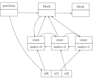
3.2.1 Data structures
partition block block
state index=0
state index=2
state index=1
s[0] s[1] s[2]
Figure 3.1: Example data structure
state. So, for large numbers of blocks using bitsets requires more memory. Therefore, we used a linked list to store the states in a block.
Each block has two flags (bits) that show its membership in L and L00. A block also has a pointer to its sub-block tree. Each state structure has a pointer to its block. The partition structure also has an array of pointers to state structures. Element s[i] in this array points to the state structure of state si. Because a state structure has a pointer to its block, this array makes it easy to access the block of a state.
3.2.2 The initial partition
States in each equivalence class (block) under bisimulation agree on their atomic propositions. Thus, states which have the same combination of atomic propositions should be put into the same block in the initial par-titionP:
∀si, sj ∈B . L(si) =L(sj) for all B ∈P
The number of different combinations of atomic propositions is 2|AP|. Ob-viously, the initial partition cannot contain more than|S| blocks.
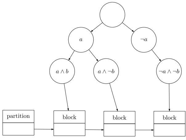
To determine in which block a state should be put, we used a binary search tree with depth |AP|. For each state si, we start at the root of this tree. If the first atomic proposition is valid in si, we move to the left subtree, otherwise we move to the right subtree. This procedure is repeated for the each atomic proposition until a leaf node is reached. This leaf node has a pointer to a block in which si should be put. The tree can be constructed while putting states in the initial partition. So, it is not necessary to build the entire tree in advance. Nodes in the tree which are never accessed are not constructed.
Figure 3.2 shows an example of such a tree. There are two atomic proposi-tionsaandb. The nodeb∧ ¬adoes not exists. So, in this example no state is labelled withb∧ ¬a.
partition block block block
a ¬a
a∧b a∧ ¬b ¬a∧ ¬b
3.2.3 Procedure LUMP
Line 1 (see Algorithm 1 on page 27) of LUMP initialises L. This set is implemented as a linked list. Every item in this list has a pointer to a block. Line 5 counts the number of blocks in the final partition. In the implementation every block is assigned a unique number which corresponds to its row index in the lumped transition matrix. Line 9 chooses an arbitrary state from a block. Our implementation simply takes the first state. Since some model checking algorithms of MRMC require the matrix values to be ordered by column index, each row (i. e. the arrays cols and vals) of the lumped transition matrix is sorted after it has been filled completely. This is done using an slightly adapted version of quicksort [1].
3.2.4 Procedure SPLIT
L0 of the SPLIT procedure stores the set of states that have a transition to a state in Sp. It is implemented as a global integer array of size |S|. The state indices j of states sj are stored in this array. A variable to maintain the number of used elements is incremented every time an element is added at line 8. Each state si is appended to L0 once, if the old value of q(si, Sp) is zero.
The values of the cumulative functionq are stored in a global array sum[ ]. Element sum[i] in this array stores q(si, Sp). Lines 2–4 initialises these values to zero for states which have a transition to a state in S. This can be replaced by setting q(si, Sp) to zero after state si has been inserted into the sub-block tree on line 12. This is allowed because q(si, Sp) is not used again after the insert into the tree. The array then only has to be initialised to zero before the first call to SPLIT. This is much faster than iterating through all predecessors.
Because MRMC uses a sparse matrix representation to store the transition matrix line 7 cannot be implemented to take constant time. The row el-ements are ordered by column so a binary search can be used to access
Q(si, sj). This takes O(logn) time, where n is the number of successor states of si, i. e. the number of non-zero elements in rowi.
The sub-block tree is implemented as a splay tree. Each tree node contains a pointer to a block structure, which is a sub-block of the original block. A tree node also contains a key equal toq(s, Sp), where sis a state contained in that sub-block. Every time a state is deleted from its original block and inserted into a sub-block, the number of states in the original block and the sub-block is updated. For this state, also the pointer to its block is updated. We used the splay tree implementation from Daniel Sleator’s website 1.
1
Lines 14–20 update the list of potential splitters. For each block B ∈ L00
the sub-blocks are added to the list of potential splitters. If B is not (yet) a potential splitter, the largest sub-block can be neglected. Each block has a flag to show its membership inL, which makes it is easy to determine if
B is already a potential splitter.
Bisimulation minimisation
and PCTL model checking
4.1
Introduction
This chapter describes experiments to study the effectiveness of bisimulation minimisation for PCTL model checking. We used several case studies from the PRISM website [26]. In these case studies, a probabilistic model of an algorithm or protocol is defined. The probabilistic model checker PRISM [22] is then used to check whether certain PCTL properties hold.
In this study, we used PRISM to build and export a DTMC for these proba-bilistic models. Using MRMC, we minimised this original model to compute a lumped model. The implementation of the lumping algorithm is described in the previous chapter. When creating the initial partition, only atomic propositions contained in the PCTL property were considered. After lump-ing, the labelling function was modified such that it corresponded to the lumped DTMC. In our experiments, the time to check the property on the original DTMC is compared to the time to lump and check the property on the lumped DTMC.
For each case study a short description will follow. Then the PCTL prop-erties are explained and finally the results are presented. These results include:
• the number of states and transitions in the original DTMC represent-ing the model;
• the number of blocks (i. e. states) in the lumped DTMC;
• MC equals the time (in milliseconds) to check the PCTL property;
• the reduction factor of the state space;
• the reduction factor of the runtime (i. e. checking the original DTMC divided by lumping plus checking the lumped DTMC).
Also the time complexity of the lumping algorithm, O(mlogn), where n is the number of states and m is the number of transition in the DTMC, is compared to the actual runtime.
All experiments were conducted on an Intel Pentium 4 2.66 GHz with 1 GB RAM running Linux.
4.2
PCTL properties
To study the effectiveness of bisimulation minimisation for PCTL model checking it is important which kind of properties to consider. Assuming states are labelled with Φ and Ψ model checking ¬Φ, Φ∧Ψ, Φ∨Ψ and
XΦ is straightforward and not computationally expensive. This leaves the bounded and unbounded until operators.
The algorithm for model checking bounded until operators is given in section 2.3.2. The state probabilities are calculated intiterations. Hence, increasing the boundt yields a longer computation time. Therefore, a realistic time bound with respect to the case study under consideration should be chosen. The worst-case time complexity of model checking a bounded until operator isO(t·(m+n)) [13].
Section 2.3.2 describes the algorithm for model checking unbounded until operators. The worst-case time complexity isO(n3) [5]. Using a backward search, the set of states is partitioned into three subsets subsets Us, Uf and Ui. IfUi is empty, no linear equation system has to be solved because the solution is already given. Ui is empty if for every state in Si either no path reaches a state in Ss or all paths reach a state in Ss. For these kind of properties, it is not likely that bisimulation minimisation takes less time than model checking the original DTMC. Therefore, unbounded until properties for whichUi=∅are not considered.
4.3
Case studies
4.3.1 Synchronous Leader Election Protocol
This case study is based on the synchronous leader election protocol in [19]. Given a synchronous ring ofN processors, the protocol will elect a leader (a uniquely designated processor) by sending messages around the ring. The protocol proceeds in rounds and is parametrised by a constantK >0. Each round begins by all processors (independently) choosing a random number (uniformly) from{1, . . . , K}as an id. The processors then pass their selected id to all other processors around the ring. If there is a unique id, then the processor with the maximum unique id is elected as the leader, and otherwise all processors begin a new round. The ring is synchronous: there is a global clock and at every time slot a processor reads the message that was sent at the previous time slot (if it exists), makes at most one state transition and then may send at most one message. Each processor knowsN.
Properties
The expected number of rounds L to elect a leader depends on N and K. For bothN = 4 andN = 5, we haveL≤3. The number of steps per round isN+ 1. This corresponds to selecting a random id (one step), and passing it around through the entire ring. In our experiments, the probability of electing a leader within three rounds has been calculated. This can be expressed in PCTL by the path formula:
trueU≤3·(N+1)elected
Since there is only one atomic proposition, the number of blocks in the initial partition is two: a block for states which are labelled with elected
and a block for states which are not labelled.
Results
Tables 4.1 and 4.2 show statistics and results for different values of N and
K.
For a given N, the number of blocks in the final partition is independent of
N = 4 original DTMC lumped DTMC reduct. factor
K states transitions MC blocks lump MC states time
2 55 70 0.02 10 0.05 0.01 5.5 0.4
4 782 1037 0.4 10 0.5 0.01 78.2 0.8 6 3902 5197 1.8 10 2.1 0.01 390.2 0.9 8 12302 16397 7.0 10 9.0 0.01 1230.2 0.8 10 30014 40013 19 10 25 0.01 3001.4 0.8 12 62222 82957 41 10 52 0.01 6222.2 0.8 14 115262 153677 85 10 100 0.01 11526.2 0.8 16 196622 262157 165 10 175 0.01 19662.2 0.9
Table 4.1: Bisimulation minimisation results for 4 processors
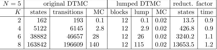
N = 5 original DTMC lumped DTMC reduct. factor
K states transitions MC blocks lump MC states time 2 162 193 0.1 12 0.1 0.02 13.5 0.9 4 5122 6145 2.8 12 2.9 0.02 426.8 0.9 6 38882 46657 28 12 26 0.02 3240.2 1.1 8 163842 196609 140 12 115 0.02 13653.5 1.2
Table 4.2: Bisimulation minimisation results for 5 processors
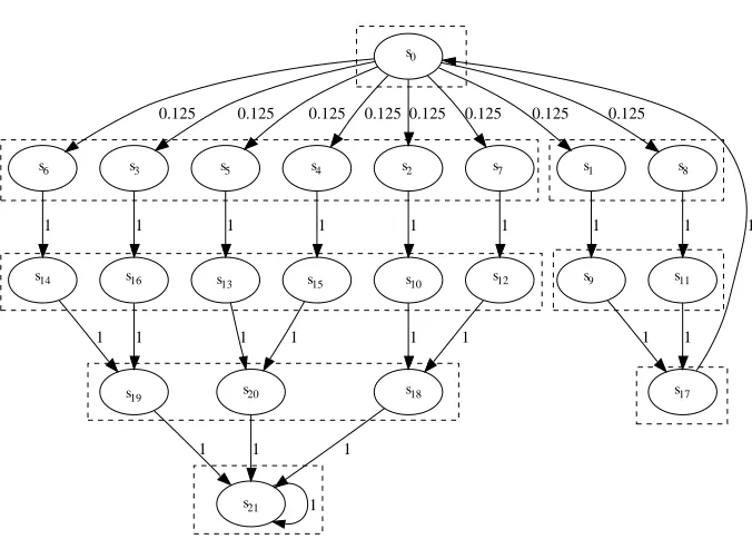
length of these paths remains equal. Therefore, all states on these paths at an equal distance from the absorbing state are bisimilar. This explains the constant number of blocks for fixedN. Figure 4.1 shows an example of this situation. States in a dashed box belong to the same equivalence class. States21 is labelled with elected.
In most cases, the time to construct the lumped DTMC exceeds the time to model check the original DTMC. The initial state is the only state which has more than one outgoing transition. Thus, only one row in the transition matrix has more than one non-zero element. Since the transition matrix is implemented as a sparse matrix, this results in a relatively low number of multiplications in each iteration when calculating the bounded until prop-erty. However, for N = 5 and K = 8, model checking the original DTMC takes longer than lumping plus model checking the minimised DTMC. In this case the number of states and transitions is less than for exampleN = 4 andK = 16, but the bound in the until property is higher, which results in more iterations and therefore a longer computation time.
To compare the actual runtime of the lumping algorithm to its time com-plexity, the value c has been calculated, where l = c mlogn (l denotes the lumping time). For most cases, this results in a nearly constant value of
s0
s6 s3 s5 s4 s2 s7 s1 s8
s14 s16 s13 s15 s10 s12 s9 s11
s19 s20 s18 s17
s21
0.125 0.125
0.125 0.125 0.125
0.125 0.125 0.125
1 1
1 1 1
1 1 1
1 1
1 1 1
1 1 1
1
1 1
1 1
Figure 4.1: Example DTMC for N = 3 and K = 2
4.3.2 Randomised Self-stabilisation
A self-stabilising protocol for a network of processes is a protocol which, when started from some possibly illegal start state, returns to a legal/stable state without any outside intervention within some finite number of steps. This case study considers Herman’s self stabilising algorithm [16]. The pro-tocol operates synchronously and communication is unidirectional in the ring. In this protocol, the number of processesN in the ring must be odd. The stable states are those where there is exactly one process which possesses a token.
Each process in the ring has a local Boolean variablexi, and there is a token at position iifxi=x(i−1). In a basic step of the protocol, if the current values ofxiand x(i−1) are equal, then it makes a (uniform) random choice as to the next value ofxi, and otherwise it sets it equal to the current value ofx(i−1).
Properties
Expressed in PCTL by the path formula:
trueU≤N2/2stable
In the initial partition the number of states labelledstable is equal toN.
Results
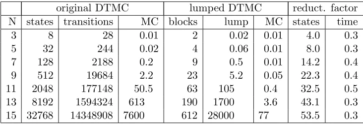
Table 4.3 shows statistics and results for different number of processesN. original DTMC lumped DTMC reduct. factor N states transitions MC blocks lump MC states time
3 8 28 0.01 2 0.02 0.01 4.0 0.3
5 32 244 0.02 4 0.06 0.01 8.0 0.3
7 128 2188 0.2 9 0.5 0.01 14.2 0.4
9 512 19684 2.2 23 5.2 0.05 22.3 0.4
11 2048 177148 50.5 63 105 0.4 32.5 0.5 13 8192 1594324 613 190 1700 3.6 43.1 0.3 15 32768 14348908 7600 612 28000 77 53.5 0.3
Table 4.3: Bisimulation minimisation results fortrueU≤N2
/2stable
We observe that the state space reductions improve with an increase ofN. Model checking the original DTMC takes much less time than lumping the DTMC. This can be explained by the fact that the number of transitions is very high compared to the number of states. This makes computing the q
value in the lumping algorithm a time consuming procedure, because this value cannot be accessed in constant time (see section 3.2.4).
Similar to the leader election case study, we calculated the value c, where
l= c mlogn. For this case study, c is not constant. As N grows, c seems to grow linearly. Hence, there is a close resemblance between the time complexity and the actual runtime.
4.3.3 Crowds Protocol
It is assumed that corrupt routers are only capable of observing their lo-cal networks. The adversary’s observations are thus limited to the appar-ent source of the message. As the message travels down a (randomly con-structed) routing path from its real sender to the destination, the adversary observes it only if at least one of the corrupt members was selected among the routers. The only information available to the adversary is the identity of the crowd member immediately preceding the first corrupt member on the path. It is also assumed that communication between any two crowd members is encrypted by a pairwise symmetric key.
Crowds is designed to provide anonymity for message senders. Under a specific condition on system parameters, Crowds provably guarantees the following property for each routing path: The real sender appears no more likely to be the originator of the message than to not be the originator. Routing paths in Crowds are set up using the following protocol:
• The sender selects a crowd member at random (possibly itself), and forwards the message to it, encrypted by the corresponding pairwise key.
• The selected router flips a biased coin. With probability 1−pf, where
pf (forwarding probability) is a parameter of the system, it delivers the message directly to the destination. With probability pf, it se-lects a crowd member at random (possibly itself) as the next router in the path, and forwards the message to it, re-encrypted with the appropriate pairwise key. The next router then repeats this step. The path from a particular source to a particular destination is set up only once, when the first message is sent. The routers maintain a persistent id for each constructed path, and all subsequent messages follow the established path.
There is no bound on the maximum length of the routing path. For sim-plicity, instead of modelling each corrupt crowd member separately, a single adversary is modeled who is selected as a router with a fixed probability equal to the sum of selection probabilities of all corrupt members.
Properties
Atomic propositionobservei denotes the adversary observed crowd member
• Eventually the adversary observed the real sender more than once:
trueUobserve0
• Eventually the adversary observed someone other than the real sender more than once:
trueUobserve,
where observe≡WN
i=1observei.
Results
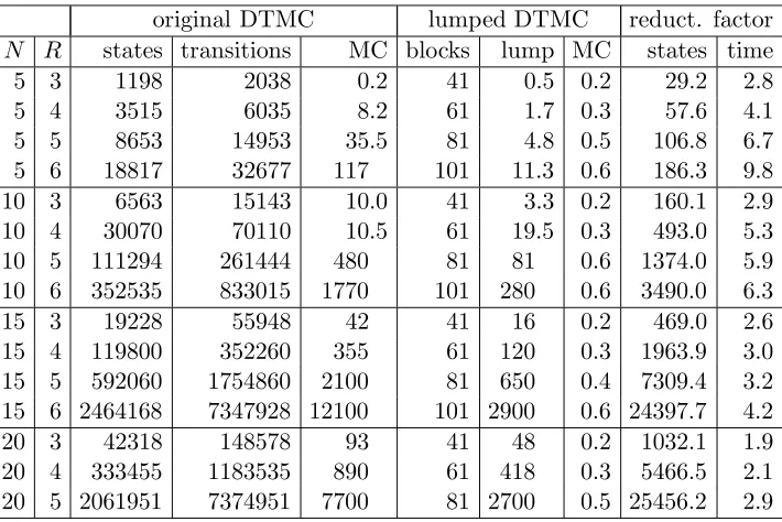
Tables 4.4 and 4.5 show statistics and results for both properties. N is the actual number of honest crowd members and R is the total number of protocol runs to analyse. ForN = 5 the number of corrupt crowd members is 1, forN = 10 the number is 2, forN = 15 the number is 3 and forN = 20 there are 4 corrupt crowd members.
original DTMC lumped DTMC reduct. factor
N R states transitions MC blocks lump MC states time 5 3 1198 2038 0.2 41 0.5 0.2 29.2 2.8 5 4 3515 6035 8.2 61 1.7 0.3 57.6 4.1 5 5 8653 14953 35.5 81 4.8 0.5 106.8 6.7 5 6 18817 32677 117 101 11.3 0.6 186.3 9.8 10 3 6563 15143 10.0 41 3.3 0.2 160.1 2.9 10 4 30070 70110 10.5 61 19.5 0.3 493.0 5.3 10 5 111294 261444 480 81 81 0.6 1374.0 5.9 10 6 352535 833015 1770 101 280 0.6 3490.0 6.3 15 3 19228 55948 42 41 16 0.2 469.0 2.6 15 4 119800 352260 355 61 120 0.3 1963.9 3.0 15 5 592060 1754860 2100 81 650 0.4 7309.4 3.2 15 6 2464168 7347928 12100 101 2900 0.6 24397.7 4.2 20 3 42318 148578 93 41 48 0.2 1032.1 1.9 20 4 333455 1183535 890 61 418 0.3 5466.5 2.1 20 5 2061951 7374951 7700 81 2700 0.5 25456.2 2.9
Table 4.4: Bisimulation minimisation results fortrueUobserve0
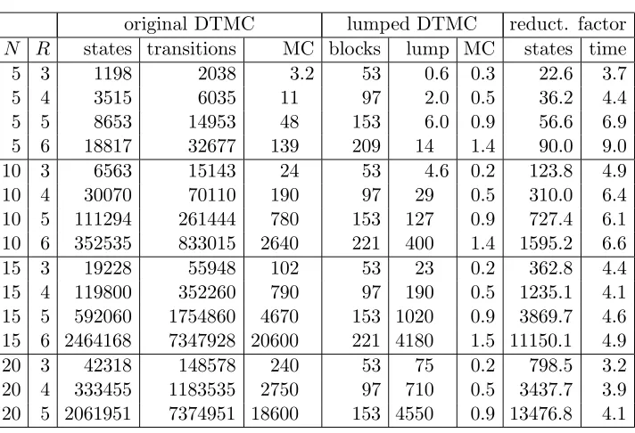
original DTMC lumped DTMC reduct. factor
N R states transitions MC blocks lump MC states time 5 3 1198 2038 3.2 53 0.6 0.3 22.6 3.7
5 4 3515 6035 11 97 2.0 0.5 36.2 4.4
5 5 8653 14953 48 153 6.0 0.9 56.6 6.9 5 6 18817 32677 139 209 14 1.4 90.0 9.0 10 3 6563 15143 24 53 4.6 0.2 123.8 4.9 10 4 30070 70110 190 97 29 0.5 310.0 6.4 10 5 111294 261444 780 153 127 0.9 727.4 6.1 10 6 352535 833015 2640 221 400 1.4 1595.2 6.6 15 3 19228 55948 102 53 23 0.2 362.8 4.4 15 4 119800 352260 790 97 190 0.5 1235.1 4.1 15 5 592060 1754860 4670 153 1020 0.9 3869.7 4.6 15 6 2464168 7347928 20600 221 4180 1.5 11150.1 4.9 20 3 42318 148578 240 53 75 0.2 798.5 3.2 20 4 333455 1183535 2750 97 710 0.5 3437.7 3.9 20 5 2061951 7374951 18600 153 4550 0.9 13476.8 4.1
Table 4.5: Bisimulation minimisation results for trueUobserve
Similar to the leader election case study, the value c has been calculated, wherel=c mlogn. For the first property, we have c∈[17,25], and for the second propertyc∈[24,33]. Thus, the time complexity is closely related to the actual runtime.
4.3.4 Randomised Mutual Exclusion
This case study is based on Pnueli and Zuck’s solution [25] to the well-known mutual exclusion problem. Let P1 . . .PN be N processes that from time to time need to execute a critical section in which at most one of them is allowed. The processes can coordinate their activities by use of a common resource. This solution guarantees at any time t there is at most one process in its critical section phase. It also guarantees if a process tries, then eventually it enters the critical section.
Properties
The state probabilities for P1 entering the critical section first have been
calculated. This can be expressed in PCTL by the path formula:
notEnter1Uenter1
Combining several atomic propositions into one atomic proposition generally yields a coarser final partition.
Results
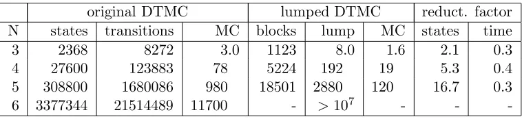
Table 4.6 shows statistics and results forN processes.
original DTMC lumped DTMC reduct. factor N states transitions MC blocks lump MC states time
3 2368 8272 3.0 1123 8.0 1.6 2.1 0.3
4 27600 123883 78 5224 192 19 5.3 0.4
5 308800 1680086 980 18501 2880 120 16.7 0.3 6 3377344 21514489 11700 - >107 - -
-Table 4.6: Bisimulation minimisation results fornotEnter1Uenter1
Lumping the DTMC takes significantly more time than model checking the original DTMC. The number of transitions in the original DTMC is rela-tively high, making lumping more computationally expensive. On the other hand, the number of iterations to solve the linear equation system is quite low. These numbers vary between 60 and 80, depending on the number of processes.
ForN = 6, lumping the DTMC was not completed within several hours. To compare the time complexity to the actual runtime of the lumping algorithm, more results have to be available.
4.4
Conclusion
The effectiveness of bisimulation minimisation for PCTL model checking has been studied. The case studies on synchronous leader election and ran-domised self-stabilisation have been used to check bounded until properties. For some configurations of the synchronous leader election protocol, lump-ing plus model checklump-ing the minimised DTMC takes less time than model checking the original DTMC. This suggests there is a lower time bound above which bisimulation minimisation is effective. However, it is hard to predict this bound exactly for concrete cases. For all other configurations as well as the randomised self-stabilisation protocol, model checking the orig-inal DTMC takes less time than lumping and model checking the lumped DTMC.
this is not the case. Randomised mutual exclusion requires a relatively low number of iterations to solve the linear equation system in comparison to the Crowds protocol. This could explain the fact that bisimulation minimi-sation is effective for the Crowds protocol, but not for randomised mutual exclusion. It should be noted that MRMC implements the Jacobi method to solve the linear equation system for PCTL unbounded until formulas. This method generally converges slower than for example the Gauss-Seidel method [30]. Using the Gauss-Seidel method could improve the runtime of model checking unbounded until properties.
The time complexity of the lumping algorithm isO(mlogn), wherenis the number of states and m is the number of transition in the DTMC. Except for the mutual exclusion case study, this time complexity has been compared to the actual runtime. For most cases, the actual runtime is closely related to the time complexity.
The experiments have shown that in some cases bisimulation minimisation is effective for PCTL properties with (at least) one until operator. For most cases it was not effective. This does not imply that bisimulation minimi-sation can play no role in PCTL model checking. It is possible to check several properties on a lumped DTMC. To do this, the DTMC has to be lumped by considering the atomic propositions contained in all properties to be checked. These properties can then be checked on a (possibly) much smaller DTMC and thus require less computation time.
Predicting in advance whether bisimulation minimisation is effective for PCTL model checking is not easy. For a parametrised model (e. g. the synchronous leader election protocol with N processors), a strategy could be to consider small cases first. If bisimulation minimisation is effective for these cases, it is likely to be effective for larger cases.
Formula-dependent lumping
for PCTL model checking
5.1
Introduction
This chapter considers formula-dependent lumping for PCTL until formulas, which might lead to more important state space reductions. This can be explained using the notion ofF bisimulation [5]. Instead of labelling states with atomic propositions, each state is labelled with formulas from a set F
that are valid in that state. So, the bisimulation relation in chapter 4 can be viewed as anAP bisimulation, which is essentially formula-independent lumping.
First, we present F bisimulation and bisimulation equivalence for PCTL. Then, we describe which PCTL properties are checked and how we can lump the DTMC for these properties. Finally, the case studies and results are presented.
5.2
Bisimulation equivalence
In [5], F bisimulation and bisimulation equivalence is defined for CTMCs and CSL. We define this for DTMCs and PCTL in a similar way.
Definition 14. Let D= (S,P, L) be a DTMC, F a set of PCTL formulas, and R an equivalence relation on S. R is an F bisimulation on D if for (s, s0)∈R:
LF(s) =LF(s0) and P(s, C) =P(s0, C) for all C∈S/R,
Definition 15. Let P CT LF denote the smallest set of PCTL formulas that includes F and is closed under all PCTL operators.
Theorem 3. Let R be an F bisimulation on DTMC D = (S,P, L) and s
ands0 states in S. Then,
1. For all P CT LF formulas Φ, (s, s0)∈R⇒ s|=DΦ↔s0 |=DΦ. 2. For all P CT LF path formulas φ,
(s, s0)∈R⇒Pr({σ ∈P athD(s)|σ |=D φ}) = Pr({σ∈P athD(s0)|σ|=Dφ}). Proof. The proof is adapted from [3] and goes by induction on the length of the formula, where formulas in F are of length 1. To avoid problems with until formulas, we transform formulas of the form Φ U≤tΨ such that Φ∩Ψ =∅. This can be done easily, as ΦU≤tΨ⇔(Φ∧ ¬Ψ)U≤tΨ.
The only state formulas of length 1 are the formulas in F. By definition of F bisimulation, the labels of bisimilar states agree. Therefore, for state formulas of length 1 the theorem holds. For path formala of length 1, this is trivial.
The induction hypothesis is: The theorem holds for all state formulas of length at most k and for all path formulas of length at mostk.
Let the induction hypothesis hold for formulas of length at mostk. We start with the proof for state formulas. Let Φ be a state formula of lengthk+ 1.
• Φ =¬Φ1or Φ = Φ1∧Φ2, where Φ1 and Φ2 are state formulas: Follows
directly from the induction hypothesis.
• Φ =PEp(φ), whereφis a path formula. From the induction hypothe-sis, we know that the probability measure of the set of states starting inswhich satisfyφequals the probability measure of the set of states starting in s0 which satisfy φ. Thus, s|=D PEp(φ)↔s0|=DPEp(φ) Now, we show the proof for path formulas. Letφbe a path formula of length
k+ 1.
• φ=XΦ, where Φ is state formula. By definition, Pr({σ∈P athD(s)| σ |=XΦ}) = X
s0|= DΦ
P(s, s0).
According to the induction hypothesis, bisimilar states agree on the same state formulas. Since states in C ∈ S/R are bisimilar, we can rewrite this as:
Pr({σ ∈P athD(s) | σ|=XΦ}) = X C|=D/RΦ
By definition of F bisimulation, bisimilar states s and s0 have the same cumulative probability of moving to any other equivalence class:
∀C ∈ S/R P(s, C) = P(s0, C). Therefore, the probability measures are equal:
Pr({σ ∈P athD(s) | σ|=DXΦ}) = Pr({σ∈P athD(s0) | σ|=DXΦ})
• φ= ΦU≤tΨ, where Φ and Ψ are state formulas. We define the set of pathsBs
n starting insthat satisfyφafter exactly nsteps as:
Bns ={σ∈P athD(s)| ∀ 0≤i < n(σ[i] |=D Φ)∧σ[n] |=D Ψ} Since the setsBs
i are disjoint, the probability measure of paths starting insis now given by:
Pr({σ ∈P athD(s)| σ|=Dφ}) = t
X
i=0
Pr(Bis)
By induction on iit can be seen that ∀iPr(Bs
i) = Pr(Bs
0
i ) [3]. From this followsPt
i=0Pr(Bis) =
Pt
i=0Pr(Bs
0
i ). Thus:
Pr({σ∈P athD(s) |σ |=Dφ}) = Pr({σ∈P athD(s0) | σ|=Dφ})
• φ= ΦUΨ, where Φ and Ψ are state formulas. This formula is equiv-alent to ΦU≤∞Ψ. Thus, the probability measure is given by:
Pr({σ ∈P athD(s) | σ |=D φ}) = ∞
X
i=0
Pr(Bns)
Note that the sum converges as Pr is a probability measure. Similar to the bounded until case, we have P∞
i=0Pr(Bis) =
P∞
i=0Pr(Bs
0
i ) [3]. Therefore, we can conclude:
Pr({σ∈P athD(s) |σ |=Dφ}) = Pr({σ∈P athD(s0) | σ|=Dφ})
We can conclude that the theorem holds for any PCTLF formula of length
k >0.
Thus, we can check each PCTL formula Φ∈PCTLF on the lumped DTMC
5.3
PCTL properties
To check bounded until formulasφ =PEp(Φ U≤tΨ), the set of states S is partitioned into three subsetsSs, Sf and Si (see section 2.3.2):
Ss = {s∈S | s|= Ψ}
Sf = {s∈S | s|=¬Φ∧ ¬Ψ}
Si = {s∈S | s|= Φ∧ ¬Ψ}
Formula φ can be checked using an F bisimulation with F = {Ψ,¬Φ∧ ¬Ψ,Φ∧ ¬Ψ}. First, we have to show that φ ∈ PCTLF. It is easy to see thatψ=PEp((Φ∧ ¬Ψ)U≤tΨ)∈PCTLF. Now, we show that φ⇔ψ. It is sufficient to show that both formulas agree on their subsets Ss, Sf and Si. This is easy to see forSs and Si. For formulaψ we have:
Sf = Sat(¬(Φ∧ ¬Ψ)∧ ¬Ψ) = Sat((¬Φ∨Ψ)∧ ¬Ψ)
= Sat((¬Φ∧ ¬Ψ)∨(Ψ∧ ¬Ψ)) = Sat(¬Φ∧ ¬Ψ)
Therefore, both formulas agree on Ss, Sf and Si. Because φ⇔ ψ, we can also checkφ using theF bisimulation mentioned above.
The initial partition corresponding to F = {Ψ,¬Φ∧ ¬Ψ,Φ∧ ¬Ψ} is P =
{Ss, Sf, Si}. It is possible to optimise by collapsing the states in Ss and
Sf into two single absorbing states ss and sf, respectively. Then, we can lump with initial partition P0 ={{s
s},{sf}, Si}. In general, lumping with
P0 instead of P yields a coarser partition. To avoid the construction of transition matrix P00 in which states from S
s and Sf are collapsed into absorbing states ss and sf, the lumping algorithm has been modified to be able to omit blocks from partitioning. Blocks which are omitted cannot be split, but will still be considered as potential splitters. To omit a block
B, lines 2–8 of the SPLIT procedure of the lumping algorithm have been modified to skip states inB. In this case, blocksSsandSf are to be omitted while lumping with P. This saves time and memory, becauseP00 does not need to be constructed explicitly.
In case of formula PEp(true U≤tΨ), the set Sf is empty yielding initial partition P ={Ss, S\Ss}. This is essentially anAP bisimulation, which is covered in chapter 4. A slight difference is that Ψ states can be collapsed into a single absorbing state prior to lumping. We do not consider these kinds of formulas here. Therefore, most case studies from chapter 4 cannot be used.
The unbounded until formula PEp(Φ UΨ) can also be checked using an
PU = {Us, Uf, Ui}. Sets Uf and Us are constructed by extending Sf and
Ss which implies Ui ⊆Si (see section 2.3.2). Similar to formula-dependent lumping for bounded until formulas, it is possible to optimise by collapsing states inUsandUf into two single absorbing states usanduf, respectively:
PU0 = {{us},{uf}, Ui}. Set Ui may contain significantly less states than
Si. Since Uf and Us can be omitted, less states have to be considered for partitioning in case of P0
U. Therefore, we will use PU0 as initial partition. States inUssatisfy P≥1(ΦUΨ), states inUf satisfyP≤0(ΦUΨ) and states
inUisatisfyP<1(ΦUΨ)∧P>0(ΦUΨ). So, we have anF bisimulation, where F ={P≥1(ΦUΨ),P≤0(ΦUΨ),P<1(ΦUΨ)∧ P>0(ΦUΨ)}. Similar to the
bounded until case, it can be seen that ∃ψ∈PCTLF. PEp(ΦUΨ)⇔ψ:
ψ = PEp
P<1(ΦUΨ)∧ P>0(ΦUΨ)U P≥1(ΦUΨ)
⇔ PEp
Φ∧ ¬Ψ
UΨ
⇔ PEp(ΦUΨ)
It is easy to see thatψ∈PCTLF, so we can check PEp(ΦUΨ) using the F bisimulation.
A possible optimisation when checking bounded until formulas is to partition the state space into subsetsSs, Uf and S\(Ss∪Uf). There exists no path from a state inUf to a state inSs. Therefore, for any states∈Uf we have
s|=P≤0(ΦU≤tΨ). Thus, states inUf can be made absorbing, which could yield less computation time. We cannot use the Us instead of Ss, because states in Us satisfy P≥1(Φ UΨ) but not necessarily P≥1(Φ U≤tΨ). This
approach can also be used when formula-dependent lumping for bounded until formulas. Then we take as initial partitionP ={Ss, Uf, S\(Ss∪Uf)}. In the following, we check bounded until formulas for the workstation cluster and cyclic server polling system case studies. These DTMCs areirreducible, i. e. for every pair of states sand s0 there exists a path from sto s0 and a path froms0tos. Hence, for these case studies we haveU
f =Sf. Therefore, this approach is not used in this chapter.
5.4
Case studies
of the adapted model checking procedure is presented (in milliseconds), de-noted lump+MC.
5.4.1 Randomised Mutual Exclusion
See section 4.3.4 for a description of this case study and the PCTL formula.
Results
Tables 5.1 show the results of formula-dependent lumping forN processes. original DTMC lumped DTMC reduct. factor
N states transitions MC blocks lump+MC states time
3 2368 8272 3.0 233 3.2 10.2 0.9
4 27600 123883 78 785 48 35.2 1.6
5 308800 1680086 980 2159 680 143.0 1.6 6 3377344 21514489 11700 554135 39800 6.1 0.3
Table 5.1: Results fornotEnter1Uenter1
Comparing these results with table 4.6 shows the number of blocks is sig-nificantly less in case of formula-dependent lumping. For N = 4 and
N = 5, formula-dependent lumping plus model checking the lumped DTMC is also faster than model checking the original DTMC as well as formula-independent lumping plus model checking the lumped DTMC. For N = 6, formula-dependent lumping completed within a reasonable amount of time in contrast to formula-independent lumping (see section 4.3.4).
5.4.2 Workstation Cluster
This case study considers a dependable cluster of workstations [15]. Two sub-cluster are connected via a backbone connection. Each sub-cluster con-sists ofN workstations, connected in a star topology with a central switch that provides the interface to the backbone. Each of the components of the system (workstation, switch, backbone) can break down. There is a single repair unit that takes care of repairing failed components. The model is represented as a CTMC.
Properties
premium are defined. Proposition minimumcorresponds to the minimum quality of service (QoS) provided: at least 34N workstations have to be op-erational and these workstations have to be connected to each other via operational switches. For premium quality of service at least N worksta-tions have to be operational, with the same connectivity constraints. N
is the number of workstations in each sub-cluster, so the total number of workstations is 2N.
The following PCTL path formulas are checked:
• Within k steps the QoS is turned fromminimumto premium:
minimumU≤kpremium
We take the bound to be k = q · t, where q is the uniformisation rate. This value q·t is equal to the expected number of steps in the uniformised DTMC corresponding to the state probabilities at timet, where t is a time instant in the original CTMC. The uniformisation rate is 51 and t= 10 is a reasonable amount of time in the CTMC of the workstation cluster. So, we havek = 510.
• The QoS turns fromminimumto premium:
minimumUpremium
Results
Tables 5.2 and 5.3 show the results of formula-dependent lumping for N
workstations. The last column of table 5.2 shows the number of blocks when using an AP bisimulation like we did in chapter 4. Obviously, for the second property these numbers are the same, since we are lumping with respect to the same atomic propositions.
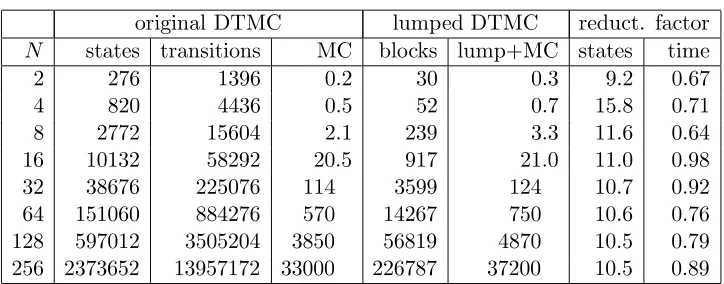
original DTMC lumped DTMC reduct. factor F =AP N states transitions MC blocks lump+MC states time blocks
2 276 1396 1.8 30 0.5 9.2 3.6 147
4 820 4436 4.6 52 1.1 15.8 4.2 425
8 2772 15604 17 239 5.7 11.6 3.0 1413
16 10132 58292 140 917 29 11.0 4.8 5117 32 38676 225076 603 3599 170 10.7 3.6 19437 64 151060 884276 2340 14267 960 10.6 2.4 75725 128 597012 3505204 9250 56819 5400 10.5 1.7 298893 256 2373652 13957172 38100 226787 36600 10.5 1.1 1187597
original DTMC lumped DTMC reduct. factor
N states transitions MC blocks lump+MC states time
2 276 1396 0.2 30 0.3 9.2 0.67
4 820 4436 0.5 52 0.7 15.8 0.71
8 2772 15604 2.1 239 3.3 11.6 0.64
16 10132 58292 20.5 917 21.0 11.0 0.98 32 38676 225076 114 3599 124 10.7 0.92 64 151060 884276 570 14267 750 10.6 0.76 128 597012 3505204 3850 56819 4870 10.5 0.79 256 2373652 13957172 33000 226787 37200 10.5 0.89
Table 5.3: Results forminimumUpremium
Table 5.2 shows formula-dependent lumping yields a significantly smaller DTMC than formula-independent lumping. Note that the reduction factor of the state space is quite constant. Formula-dependent lumping plus model checking the lumped DTMC for the first property is faster than checking the original DTMC. For the second property, checking the original DTMC is slightly faster. This can be explained by means of the number of iterations to solve the linear equation system. AsN increases, the number of iterations also increases. This number is at most 325, forN = 256. Thus, the number of iterations is significantly lower thank. Hence, the computation time of the unbounded until property is less.
We observe that, for a givenN, the number of blocks for both properties is equal. So unfortunately, lumping with initial partitionPU0 ={{us},{uf}, Ui} does not lead to a coarser partition than lumping with initial partition
P0 ={{s
s},{sf}, Si}.
5.4.3 Cyclic Server Polling System
This case study is based on a cyclic server polling system [18]. It consists of one polling server which handles N stations. Each station has a buffer. The polling server polls the stations in a cyclic manner. If a station has a full buffer, the station is served by the server. After this, the buffer is empty again and the server continues polling the stations. The model is represented as a CTMC.
Properties
The following PCTL path formulas are checked:
• Within k steps station 1 is served before all other stations:
notServe1U≤tserve1
We take k=q·t, like in the previous case study. The uniformisation rate is 202 and t= 5, so we have k = 1010.
• Station 1 is served before all other stations:
notServe1 Userve1
Atomic propositionsnotServei is defined as: notServei ≡VNj6=i¬servej. In the original case study, the authors check the formula ¬serve2Userve1.
We find the formulanotServe1Userve1 more intuitive, since this expresses
whether station 1 is served first, instead of only earlier than station 2.
Results
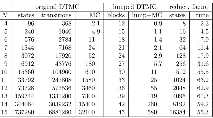
Tables 5.4 and 5.5 show the results of formula-dependent lumping for N
stations.
original DTMC lumped DTMC reduct. factor
N states transitions MC blocks lump+MC states time
4 96 368 1.4 19 0.4 5.1 3.5
5 240 1040 4.2 26 0.7 9.2 6.0
6 576 2784 10 34 1.2 16.9 8.3
7 1344 7168 25 43 2.0 31.3 12.5
8 3072 17920 62 53 4.0 58.0 15.5
9 6912 43776 190 64 9.4 108.0 20.2
10 15360 104960 575 76 22 202.1 26.1
11 33792 247808 1310 89 51 379.7 25.7 12 73728 577536 3050 103 120 715.8 25.4 13 159744 1331200 7250 118 287 1353.8 25.3 14 344064 3039232 16900 134 730 2567.6 23.2 15 737280 6881280 39000 151 1590 4882.6 24.5
Table 5.4: Results fornotServe1 U≤1010serve1
original DTMC lumped DTMC reduct. factor
N states transitions MC blocks lump+MC states time
4 96 368 2.1 12 0.9 8 2.3
5 240 1040 4.9 15 1.1 16 4.5
6 576 2784 11 18 1.4 32 7.9
7 1344 7168 24 21 2.1 64 11.4
8 3072 17920 52 24 2.9 128 17.9
9 6912 43776 180 27 5.7 256 31.6
10 15360 104960 610 30 11 512 55.5
11 33792 247808 1580 33 25 1024 63.2
12 73728 577536 3460 36 55 2048 62.9
13 159744 1331200 7300 39 119 4096 61.3 14 344064 3039232 15400 42 260 8192 59.2 15 737280 6881280 32100 45 580 16384 55.3
Table 5.5: Results fornotServe1Userve1
Also, the number of blocks in case of the second property is significantly less compared to the first property. So, for this case study, lumping with initial partition P0
U = {{us},{uf}, Ui} does lead to a significantly coarser partition than lumping with initial partitionP0 ={{ss},{sf}, Si}. Finally, for both properties, formula-dependent lumping plus model checking the lumped DTMC is faster than model checking the original DTMC.
5.5
Conclusion
The effectiveness of formula-dependent lumping for PCTL bounded and unbounded until formulas has been studied. An advantage of formula-dependent lumping is that some blocks in the initial partition can be omitted yielding a shorter lumping time. A disadvantage is that the lumped DTMC cannot be reused for model checking formulas in which the until formula is not contained. The DTMC is lumped with respect to a specific until formula. This is the main difference with formula-independent lumping. Three case studies have been used: randomised mutua