Volume 2009, Article ID 469480,17pages doi:10.1155/2009/469480
Research Article
Improved Reproduction of Stops in Noise Reduction Systems with
Adaptive Windows and Nonstationarity Detection
Dirk Mauler and Rainer Martin (EURASIP Member)
Department of Electrical Engineering and Information Sciences, Ruhr-Universit¨at Bochum, 44801 Bochum, Germany
Correspondence should be addressed to Dirk Mauler,[email protected]
Received 12 December 2008; Accepted 17 March 2009
Recommended by Sven Nordholm
A new block-based noise reduction system is proposed which focuses on the preservation of transient sounds like stops or speech onsets. The power level of consonants has been shown to be important for speech intelligibility. In single-channel noise reduction systems, however, these sounds are frequently severely attenuated. The main reasons for this are an insufficient temporal resolution of transient sounds and a delayed tracking of important control parameters. The key idea of the proposed system is the detection of non-stationary input data. Depending on that decision, a pair of spectral analysis-synthesis windows is selected which either provides high temporal or high spectral resolution. Furthermore, thedecision-directedapproach for the estimation of the a priori SNR is modified so that speech onsets are tracked more quickly without sacrificing performance in stationary signal regions. The proposed solution shows significant improvements in the preservation of stops with an overall system delay (input-output, excluding group delay of noise reduction filter) of only 10 milliseconds.
Copyright © 2009 D. Mauler and R. Martin. This is an open access article distributed under the Creative Commons Attribution License, which permits unrestricted use, distribution, and reproduction in any medium, provided the original work is properly cited.
1. Introduction
A large class of speech enhancement algorithms is realized in the spectral domain. Since their performance depends on the quality of the spectral representation of the noisy data, sys-tems for a reliable and precise spectral analysis are required. Apart of filter bank implementations, a common approach is to compute the discrete Fourier Transform (DFT) on short overlapping time domain segments [1]. Short-time DFT systems with frame overlap are attractive because of their aliasing robustness and ease of implementation [2]. The data length of a short-time segment is on the one hand connected to the frequency resolution which is achieved after transfor-mation. The longer the time domain segment, the higher the spectral resolution. A short data length, on the other hand, is required for a good temporal resolution. In noise reduction systems usually a fixed data length is used for the short-time spectral analysis, thus making a compromise between the required spectral resolution and the minimal admissible temporal resolution [3, page 469]. This concept, however, has a major drawback: in order to achieve a sufficiently high frequency resolution, in many noise reduction systems the
the time domain data prior to the computation of the short-time DFT. The disadvantages of this method are its high computational demands and the fact that the extrapolation requires perfect modeling of the signal which is in general difficult to achieve. Furthermore, random noise cannot be properly extrapolated. In audio coding, analysis windows of different lengths and shapes are switched in a signal-dependent fashion [6,7] in order to reduce pre-echo effects that may appear after decoding.
In many application fields like telecommunications or hearing instruments the system delay is of great importance. The group delay of a hearing instrument can produce a noticeable or even objectionable coloration of the hearing aid wearer’s own voice. In [8] it is reported that a delay of 3 to 5 milliseconds was noticeable to most of a group of normal hearing listeners while a delay of longer than 10 milliseconds was objectionable. In [9] asymmetric windows are presented as a way to reduce the delay in spectral analysis. However, spectral synthesis is not discussed and would become difficult with the proposed asymmetric windows if perfect or nearly perfect reconstruction is required. The delay issue has also been addressed recently in [10] where a warped analysis-synthesis filter bank for speech enhancement is presented which achieves a very low system delay. In a DFT-based analysis-synthesis system using overlap-add for signal synthesis, the delay is given by the frame length of the synthesis window, the frame advance and the group delay of a possible spectral modification filter.
In this contribution we propose an analysis-synthesis overlap-add framework that uses different analysis-synthesis window pairs. They differ in their length (before zero-padding) and their shape. Depending on the stationarity of the current time domain signal a proper window pair is selected for the analysis and synthesis. Data that is stationary over a relatively long span is analyzed using a long window in order to allow for a high spectral resolution, while short-time stationary data-like bursts of stops or speech onsets are analyzed with a short data window so that the energy burst is well preserved in the spectral representation. The reduced spectral resolution that results from using a short analysis window is not considered as a limitation, since for the latter class of short burst-like signals we expect relatively broadband spectra with few spectral details. The proposed system achieves perfect reconstruction and produces the same low delay irrespective of the analysis-synthesis window pair that is currently in use.
The signal dependent selection of an analysis-synthesis window pair to be used requires the knowledge of the span of stationarity in the signal. In order to find the boundaries of signal stationarity in [4] an iterative window growing algo-rithm is proposed that is based on a probabilistic framework. Since a necessary condition for stationarity is an invariant power of the random process, the temporal evolution of the mean power of consecutive frames is observed. Based on a likelihood ratio test a decision is made whether a neighboring frame contains data that originates from the same statistical process or not. The method requires a look-ahead over several frames of data in order to be able to determine the parameters of parameterized probability density functions
(pdfs). It is thus not suited for very low delay applications. In an alternative approach [11] the detection of stationarity changes is based on an autoregressive signal model. For the reliable estimation of the model parameters a look-ahead of 20 ms is required which again is not permissible for very low delay applications that this paper focuses on. The approach presented here allows the detection of stationarity changes with a very low delay of about 2 ms.
Eventually, we propose and evaluate a noise reduction system that integrates the switching of the analysis-synthesis window pair based on the detection of stationarity changes in the time domain signal. The information on stationarity boundaries can be used to additionally improve the preser-vation of stops and speech onsets: we propose a change of the decision-directed a priori SNR estimator [12] and the amplification of plosive-like sounds. The latter is motivated by the fact that the improvement of the consonant-vowel intensity ratio was shown to be important for improving speech intelligibility [13–15].
In Section 2 we introduce the concept of switchable analysis-synthesis window pairs and estimate the benefit and the computational cost of the approach. Then, inSection 3, we introduce a detector for stationarity changes in the time domain signal that is based on a likelihood ratio test (LRT). The analysis of the properties of the likelihood ratio helps setting a proper threshold for the LRT. InSection 4a noise-reduction system is proposed and analyzed that makes use of the nonstationarity detection. Apart from switching the analysis and synthesis windows we propose two measures that aim at improving speech intelligibility by a preservation or amplification of speech onsets and burst-like sounds. Finally, inSection 5we present experimental results.
2. Analysis-Synthesis Window Sets
In this section we define the spectral analysis-synthesis system that provides spectral data to the frequency domain noise reduction algorithm and synthesizes the time domain signal after possible spectral modifications.
The main idea in this section is to provide an analysis system with long and short analysis windows that are arbi-trarily switchable. This allows a signal dependent selection of the appropriate analysis window. Each analysis window is matched with a particular synthesis window that guarantees perfect reconstruction for each window pair.
2.1. DFT-Based Analysis Synthesis System. We assume a sampled noisy signal that is the sum of a speech signal,s(i), and uncorrelated noise,n(i)
y(i)=s(i) +n(i). (1)
The index i denotes the discrete time index of the data, sampled with sampling frequency fs.
We consider a block-based analysis-system with K
(FFT) algorithm. Then, the spectral coefficients,Yk(m), of the sampled time domain datay(i) are obtained as
Yk(m) =
K−1
i=0
x(mR + i)h(i)e−2kπi/K , (2)
whereh(i) denotes an analysis window,mis the subsampled (frame) index,k = 0. . . K−1 is the discrete frequency bin index, andKis the length of the DFT.
The spectral coefficients,Yk(m), may then be weighted with a spectral gain, Gk(m), before the signal synthesis is performed via IDFT, multiplication with a synthesis window,
f(i), and a subsequent overlap-add operation [1].
2.2. Switchable Analysis-Synthesis Window Sets. In [16] a system with switchable analysis-synthesis window pairs is proposed which achieves perfect reconstruction and can provide spectral or temporal resolution in a flexible manner while always realizing the same small delay. The main ideas that are underlying the window design are the following.
(i) Since the spectral and temporal resolution of an anal-ysis system is governed by the length of theanalysis
window, analysis windows of different lengths have to be provided for a system with maximum flexibility. (ii) The delay in an overlap-add system is basically
determined by the length of the synthesis window. Therefore, in order to realize the same short delay for all window pairs in a switchable analysis-synthesis system, the synthesis windows have to be of the same length regardless of the length of the associated analysis window.
(iii) In order to allow for an arbitrary frame-by-frame switching between different analysis-synthesis win-dow pairs, in an overlap-add system the product of analysis and associated synthesis window has to be the same for all window pairs.
(iv) The analysis-synthesis system should be perfectly reconstructing whenever no processing is applied. (v) The windows shall have reasonable frequency
re-sponses to avoid aliasing and imaging distortions.
For the subsequent investigations we use the window set example in Figure 1 [16]. It is designed for a K =
512 point DFT with frame advance R = 32 samples at 16 kHz sampling frequency and consists of two analysis-synthesis window pairs. The first window pair consists of a zero-padded square-root Hann window of length 128 (M=64 inFigure 1) for both, analysis,hI(i), and synthesis
window,fI(i). The product of analysis and synthesis window
is a length-128 Hann window. The second window pair provides an asymmetric analysis window,hII(i), with square
root Hann slopes. The long asymmetric analysis window is padded withd = 64 zeros to alleviate spectral aliasing. The respective short synthesis window, fII(i), is designed
in a way that the product of analysis and synthesis window again results in the same length-128 Hann window as for the short window pair. Therefore, an arbitrary switching
between either of the window pairs is possible without violating perfect reconstruction, of course assuming that the signal is not modified otherwise.
2.3. Analysis of Energy Gain Using Switched Windows. As mentioned before, short analysis windows provide a high temporal resolution. This implies that the energy of nonsta-tionary signal sections, like bursts of plosive speech sounds, is better captured with a short analysis window than with a long one. In the following, we quantify this effect.
A gain Gswitch can be defined as the ratio of the signal
power captured under the short analysis window, hI(i),
related to the power that would be captured under the long analysis window,hII(i)
Gswitch=
K−1 i=0
y(i)hI(i)/K−1 j=0hI2
j2
K−1 i=0
y(i)hII(i)/K−1 j=0hII
2 j2
. (3)
The windows in the numerator and denominator of the above formula are normalized to unity power. SinceK−2M
zeros are padded in window hI(i) the outer sum in the
numerator can start ati=K−2M.
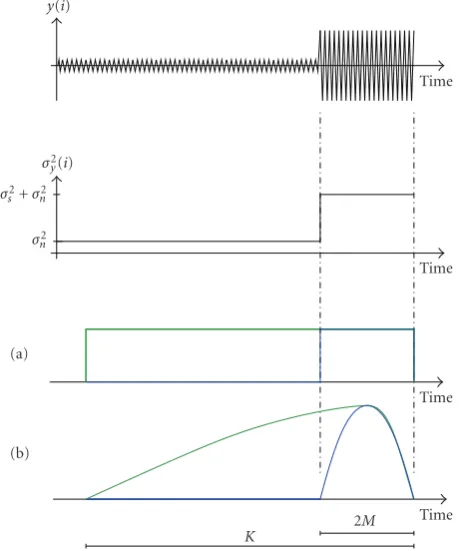
In the best case the nonstationarity (e.g. speech onset) occurs like a step function and coincides exactly with the limits of the short window, therefore maximizing the power that can be captured under the short window. This scenario is illustrated inFigure 2, whereσ2
y(i),σs2, andσn2denote the
power of the noisy signal, the speech power, and the noise power, respectively.
Speech is assumed to be statistically independent of the noise process and appears only during the 2M most recent samples. If additionally the windows hI(i) and hII(i) are
assumed to be rectangular (Figure 2(a)), (3) simplifies so that an estimate for the maximal achievable gain is
Gswitch= K/(2M)
(K/(2M)−1)σn/2 σ2 s +σn2
+ 1. (4)
In Figure 3 this expression is evaluated as a function of the a priori SNR ξ = σ2
s/σn2 and for several ratios of
the length of the short window to the length of the long window. The solid lines show the result for the assumed rectangular windows, the dashed lines show the expected gain if the proposed tapered windows of Figure 2(b) are used instead. The gain of the tapered windows is always smaller than that obtained with rectangular windows. We find that using the proposed short window over the proposed long window during a burst-like speech sound at 15 dB
a prioriSNR improves the spectral representation by roughly 4 dB. Rectangular windows would yield a gain of about 5.6 dB at these conditions. Due to their unfavorable spectral properties rectangular analysis windows do not represent an alternative but should instead serve here as the upper bound for possible gains,Gswitch. Note that an increase in the
0 0.5 1
Short analysis window
0 64 128 192 256 320 384 448 512
d K−2M−d M M
hI(i)
(a)
0 0.5 1
Long analysis window
0 64 128 192 256 320 384 448 512
d K−2M−d M M
hII(i)
(b)
0 0.5 1
Short synthesis window
0 64 128 192 256 320 384 448 512
d K−2M−d M M
fI(i)
(c)
0 0.5 1
Long synthesis window
0 64 128 192 256 320 384 448 512
d K−2M−d M M
fII(i)
(d)
Figure1: Example for a low delay switchable analysis-synthesis window set guaranteeing perfect reconstruction. The window pair in the left column has good temporal resolution while the pair in the right column provides a good spectral resolution. The asymmetry of the long analysis window emphasizes most recent samples.
In the preceding analysis we assumed that the non-stationarity coincides exactly with the limits of the short window. If this is not the case, the gain Gswitch decreases.
Therefore it is advisable to operate the analysis system with a small frame advance R. For the proposed window set in Figure 1 a choice of R = M/2 turned out to be a good compromise between computational complexity and a sufficient high temporal resolution. In terms of the filter-bank interpretation of a DFT analysis system a small frame advance corresponds to an oversampled system which is also frequently used to reduce aliasing effects [1, page 339].
2.4. Computational Complexity. For the ease of use of a flexible spectral analysis-synthesis system it is desirable that the system behaves transparently to the spectral domain application when switching from one to another window pair. The system is therefore required to always provide the same number of spectral components no matter which window set is active. For this reason all analysis windows are zero-padded to the same length so that a DFT of one and the same length can be computed. Zero-padding the short window does not increase the spectral resolution but corresponds to an interpolation of the spectral data of the short window. This increases the computational complexity as compared to the case of a standard system with a short analysis window without zero-padding but allows for a more flexible allocation of temporal and spectral resolution. Compared to a standard long window for analysis and
synthesis the proposed solution is less complex, more flexible in terms of spectrotemporal resolution and has a lower delay. With these considerations, the total number of multipli-cations can be estimated for the following three cases.
(a) Standard system with symmetric short analysis and short synthesis windows, for example, square-root Hann windows.
(b) Proposed flexible analysis-synthesis system with a set of two window pairs:
(1) short analysis window and short synthesis win-dow,
(2) long (asymmetric) analysis window and long (asymmetric) synthesis window.
(c) Standard system with symmetric long analysis and long synthesis windows, for example square-root Hann windows.
Complexity is determined here in terms of the number of real-valued multiplications. These have been determined in [17] for the calculation of an N-point FFT or IFFT:
C(N)=0.5Nlog2N−1.5N+ 2. (5)
Time
Time
Time
Time
y(i)
2M K
σ2
y(i)
σ2
s +σn2
σ2
n
(a)
(b)
Figure2: Idealized scenario of a speech onset of powerσ2
s in noise of powerσ2
n. The speech onset coincides with the short spectral analysis window (2Mmost recent samples). The analysis window is either (a), rectangular, or (b), tapered.
toC(K). However, as most of the input data to the FFT is zero, advanced techniques for pruned FFT may reduce the complexity by a factor of [18]
r=1− l
q, (6)
where 2q = K and 2l = 2M. Further multiplications are
required when weighting the input data with the analysis window and the processed data with the synthesis window. Here, only the nonzero samples of every window have to be multiplied with the data.
Table 1 reports the computational complexity relative to the complexity of case a. Furthermore, the temporal resolution, the frequency bin spacing and the system delays are indicated for a sampling frequency of fs = 16 kHz and for a frame advance ofR = 32 samples which corresponds to 2 milliseconds. The relative computational complexity of the proposed solution varies between 3.9 and 4.7 depending on how frequently the short analysis window or the long asymmetric analysis window is used. In case a, the system delay is only 10 milliseconds. However, when applying the short window set A to a noise reduction system the denoised speech and the residual noise sound harsh and unnatural. In case b, the system delay is also low, but during longer stationary signal sections like vocals or speech pauses, the long asymmetric window can be used, resulting in a more natural sounding speech and residual noise. The short
0 2 4 6 8 10 12
Gsw
it
ch
(dB)
−15 −10 −5 0 5 10 15 20 25 30
a prioriSNRξ=σs2
σ2
n (dB) Rectangular windows
Proposed tapered windows
32/512
64/512
128/512
256/512
Figure3: Expected spectral power gain versusa prioriSNRξ for using a short analysis window versus a long window during speech onsets. The curves are labeled with the ratio of the lengths of short and long windows, 2M/K. The solid line shows the results for rectangular analysis windows, the dashed line the results for the proposed window set. The envelope of the time domain signal is idealized as a step function where the section with increased power coincides with the boundaries of the short window.
window pair in case b should be applied during transitions or during bursts of a stop. Since in speech, and in partic-ular in speech pauses, stationary signal sections dominate transient sections the long analysis-synthesis window set will be more frequently used than the short window set so that an effective relative computational complexity close to 4.7 can be expected. While the computational complexity increases when using the proposed solution B instead of A, it provides a considerably improved frequency bin spacing (about 36 Hz/bin) which principally allows to resolve pitch harmonics. A similar high resolution is obtained in case c only at the price of a much greater system delay and an even slightly higher computational complexity.
3. Detecting Stationarity Boundaries
In this section we develop a detector for stationarity boundaries of data which controls the selection of windows to be used for the spectral analysis of the current segment. Since for a real-time application this decision has to be made frame-by-frame, the detector is optimized for decisions with very low latency. This is an important aspect in which our solution differs from other approaches which use statistical models whose free parameters need to be estimated over several frames [4], or, in [11] a sufficient number of samples is required, corresponding to at least 20 ms. The algorithm presented in the following is operating on the time domain sampled data. It gives also information on how reliable the stationarity-decision is.
Table1: Comparison of proposed window set (center column) with a standard analysis-synthesis system using short (left column) or long (right column) standard analysis and synthesis windows. The values are indicated for a sampling frequencyfs=16 kHz and a frame advance ofR=32 samples (2 ms). The effective complexity of the proposed solution varies between 3.9 and 4.7 depending on the rate of use of either the short or the long analysis window. Typically, the long analysis window will be used more frequently than the short analysis window.
A) standard B) proposed solution of switchable C) standard
short symm. analysis window short symm. synthesis window
short symm. analysis window
short symm. synthesis window
short symm. analysis window
long asymm. synthesis window
long symm. analysis window long symm. synthesis window
DFT length 128 512 512
Zero-padding 0 384 64 0
Effective window length 128 128 448 512
Complexity 1.0 3.9· · ·4.7 5.3
Temporal resolution 8 ms 8 ms 32 ms 32 ms
Frequency bin spacing 125 Hz/bin 125 Hz/bin 36 Hz/bin 31.25 Hz/bin
System delay (8+2) ms (8+2) ms (32+2) ms
Time Block 1
K1
Block 2
K2
Figure4: Definition of blocks 1 and 2, consisting ofK1 and K2
samples, respectively.
same statistical process as the K1 preceding samples (block
1). Thus, we have the following hypotheses:
H0: the samples in block 2 originate from the same
statistics as those ones in the preceding block 1, that is, the data is stationary over both blocks;
H1: the samples in block 2 are supposed to follow
different statistics than the samples in block 1 (detection of a stationarity boundary between the two blocks of data).
The lengthsK1andK2can be arbitrarily set. A necessary
condition for stationarity is that the process mean power must be constant over time. We inherently assume ergodicity of the random processes in the respective blocks of data since we replace the ensemble mean by the mean over the consecutive observations (e.g., squared time domain samples) within the respective blocks.
Furthermore, it is assumed that the samples within each of the two blocks are independent identically distributed (i.i.d.) and are wide-sense stationary within each block. This assumption may be violated, for example, during voiced speech or when the boundary between block 1 and block 2 does not coincide with the stationarity boundary. In practice, however, it turns out that with a proper parameter setting
of the detector the stationarity detection works well even in these cases.
3.2. Likelihood-based Hypothesis Test. The hypothesis is tested with a likelihood ratio test (LRT). This requires the knowledge of the probability density function (pdf) which describes the distribution of the squared samples in block 1 and 2 under hypothesisH1orH0.
Assuming that the observed time domain samples, y(i), are realizations of a zero-mean Gaussian random variable with variance σ2
Y, then the squared observations, y2(i), are
χ2distributed withN =1 degree of freedom [19, Equations
(5.33), (5.65)]
pW(ω)=
1 2πμWω
exp
− ω
2μW
, ω >0, (7)
and pW(ω) = 0 for ω ≤ 0. The mean of the squared
random variable, μW, is the variance of the noisy
time-domain samples,μW=σY2.
Given hypothesis H0, the data in both blocks originate
from the same statistical process, so that the pdf describing the distribution of the squared samples in block 2 can be formulated using the variance of the noisy time-domain samples in block 1,σ2
Y1:
pW|H0(ω|H0)=
1
2πσ2
Y1ω
exp
− ω
2σY21
, ω >0. (8)
If, on the other hand, the data in block 2 originate from a different statistics than the data in block 1 (hypothesisH1),
the mean power has to be defined using only data of block 2:
pW|H1(ω|H1)=
1
2πσ2
Y2ω
exp
− ω
2σY22
, ω >0. (9)
The variance of the noisy observations in block 1 and 2 constitute random variables, which may be approximated by their respective maximum likelihood estimates
σ2
Y1=
1
K1 K1−1
k=0
y2(i−k−K
2), (10)
σ2
Y2=
1
K2 K2−1
k=0
y2(i−k). (11)
Given the squared observations in block 2, y2(i), a
likelihood ratio (LR) test is defined by
ΠK2−1
k=0 pW|H0(ω|H0)|ω=y2(i−k)
ΠK2−1
k=0 pW|H1(ω|H1)|ω=y2(i−k) H0
≷ H1
λ, (12)
=⇒LR= σY2
σY1
exp −1 2 σ2 Y2 σ2 Y1 −1 H0 ≷ H1
λ, (13)
withλ=λ1/K2 being the LR decision threshold to be set to
a reasonable value from the interval of possible LR values, [0, 1].
The LR value gives an indication whether the observed mean energyσ2
Y2could have originated from both
distribu-tions with equal or similar likelihood (LR> λ) or whether the statistics are significantly different. In the latter case we rejectH0 and decide that a stationarity boundary has been
detected, in the former case we accept H0 as we have no
sufficient evidence that stationarity has been violated. The LR value itself gives information on the reliability of the decision. The more it approaches zero, the more reliable is the decision forH1. Accordingly, values close to one indicate
a highly reliable decision forH0.
The value of the decision thresholdλcontrols the trade offbetween detection and false alarm rates. The higherλthe more stationarity boundaries are detected at the cost of an increased false alarm rate. In the next section we analyze the LR expression and investigate the relation between threshold
λand the probabilities of detection and false alarm.
3.3. Analysis of the Likelihood Ratio. In the sequel an expression will be derived for the likelihood ratio as a function of the SNR in the first block of data and the change of the SNR at the transition from block 1 to block 2. The analysis of the expected LR values and their variance helps to properly set the detection thresholdλ.
3.3.1. Expected LR Value. Assuming speech and noise being statistically independent random variables with σS2 andσN2
being their respective variances, then the observed signal
y(i)=s(i) +n(i) has varianceσ2
Y =σS2+σN2. Therefore, the
variances in block 1 and 2 may be written as
σ2
Y1=σ
2
S1+σ
2
N1=(ξ1+ 1)σ
2
N1, σ2
Y2=σ
2
S2+σ
2
N2=(ξ2+ 1)σ
2
N2,
(14)
with ξi = σ2
Siσ
2
Ni(i = 1, 2) being the a priori SNR . With
these relations the LR (13) can be written as a function of
0.1 0.2 0.2 0.3 0.3 0.4 0.4 0.5 0.5 0.6 0.6 0.7 0.7 0.8 0.8 0.9 0.9 0.9
1 1 1
−40 −30 −20 −10 0 10 20 30 40
ξ1→
2
(dB)
LR
−40 −30 −20 −10 0 10 20 30 40
ξ1(dB)
0 0.1 0.2 0.3 0.4 0.5 0.6 0.7 0.8 0.9 1
Figure5: Contour plot of the simplified likelihood ratio (16). The noise is assumed to be stationary (σ2
N2=σ
2
N1).ξ1denotes thea priori
SNR in block 1,ξ1→2the step of thea prioriSNR at the transition
from block 1 to 2.
thea prioriSNR in block 1,ξ1, and the change of the SNR at
the transition from block 1 to block 2,ξ1→2=ξ2/ξ1:
LR=
ξ1→2ξ1+ 1 ξ1+ 1
σN2 σN1
exp
−1
2
ξ1→2ξ1+ 1 ξ1+ 1
σ2
N2 σN21
−1
.
(15)
If the additive noise is stationary over both blocks 1 and 2, that is,σ2
N1=σ
2
N2, the likelihood ratio simplifies to
LR=
ξ1→2ξ1+ 1 ξ1+ 1
exp
−1
2
ξ1→2ξ1+ 1 ξ1+ 1 −
1
. (16)
Figure 5 illustrates the LR (16). The following conclu-sions can be drawn.
(i) Detection of an SNRincrease(ξ1→2>0 dB):
(1) the more the SNR ξ1 is below 0 dB the
higher has the SNR step to be in order to produce noticeable small LR values. However, the steepness of the LR function, that is, the decrease of the LR value as a function of the SNR step at a constant SNRξ1is similar for all
SNRξ1;
(2) at SNRξ1>5 dB, the LR shows similar
sensitiv-ity for SNR increases.
(ii) Detection of an SNRdecrease(ξ1→2<0 dB):
(1) below 0 dB SNR ξ1 a detection of an SNR
decrease is impossible. This is plausible as an SNR decrease of a signal that is already severely disturbed (ξ1 <0 dB) does not result in a
0. 1
0.1 0.
2
0.2
0.3
0.3 0.4
0.4 0. 5 0. 5
0.6
0. 6
0.7 0. 7
0.8
0.8
0. 9 0. 9
−40
−30
−20
−10 0 10 20 30 40
ξ1→
2
(dB)
LR
−40 −30 −20 −10 0 10 20 30 40
ξ1(dB)
0 0.1 0.2 0.3 0.4 0.5 0.6 0.7 0.8 0.9 1
Figure6: Contour plot of the likelihood ratio (15) assuming a noise power rise from block 1 to block 2 (σ2
N2 = 4σ
2
N1).ξ1denotes the
a prioriSNR in block 1,ξ1→2 the step of thea prioriSNR at the
transition from block 1 to 2.
(2) for all SNRξ1>10 dB the LR values decrease in
a similar manner overξ1→2but less steeply than
for the case of the detection of SNR increase; (3) we observe a saturation of the LR values at a
level that increases with decrease in the SNR
ξ1. For example, at an SNR ofξ1 = 10 dB an
expected LR value less than 0.48 is not possible, irrespective of the magnitude of the SNR drop.
In (16) (cf. Figure 5) noise is assumed stationary over blocks 1 and 2 which is not always the case, for example in case of babble or cafeteria noise. Figure 6shows the LR function for an assumed noise power increase by 6 dB at the transition from block 1 to block 2. During a speech pause the SNR is already very low (e.g.ξ1 <−10 dB) and a noise
burst further degrades the SNR (ξ1→2 < 0 dB). In this case
the LR function returns smaller values than in the case of stationary noise (cf.Figure 5). Therefore, depending on the level of the decision threshold λthe detector might trigger on the noise burst. This example illustrates that the detector detects any instationarities and cannot distinguish between speech or noise.
3.3.2. Variance of the LR Values. The variances of the mod-elled random processes, σ2
Y1 and σ
2
Y2, have to be estimated
from the given data (cf. (10), (11)). As a consequence the LR is a random variable with mean and variance. Since LR is a transcendental function of the random variablesσY21and
σY22, an analytic expression for the pdf of the LR is difficult to
derive. In the following we therefore simulate the LR values for normal distributed input data y(i) and determine the histograms of the LR for a given SNRξ1in block 1 and for
a given SNR stepξ1→2at the transition from block 1 to block
2. InFigure 7five histograms are plotted for five SNR steps,
ξ1→2, and constant SNRξ1. We observe that the variance of
0 0.05 0.1 0.15 0.2 0.25 0.3 0.35 0.4 0.45 0.5
R
elati
ve
fr
equency
12 dB
6 dB
−12 dB −6 dB 0 dB
0 0.1 0.2
0.3 0.4 0.5
0.6 0.7 0.8 0.9 1
LR
ξ1→2=12 dB
ξ1→2=6 dB
ξ1→2=0 dB
ξ1→2= −6 dB
ξ1→2= −12 dB
Figure7: Histograms of the LR values for constant SNRξ1=5 dB.
The amplitudes of the time-domain signal are Gaussian i.i.d. The distribution is broadest at an SNR increase between roughly 0 and 10 dB.
the data is particularly large forξ1→2=6 dB (light blue) and
is small for the casesξ1→2=0 dB (green) andξ1→2=12 dB
(dark blue).
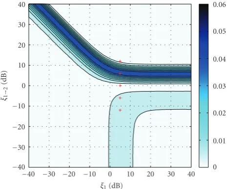
We measured the variance of the distributions of the LR values not only for the five exemplary distributions in
Figure 7, but for each pair ofξ1∈[−40, 40] dB andξ1→2 ∈
[−40, 40] dB with a resolution of 1 dB. The result is presented as a contour plot inFigure 8. The crosses indicate the five SNR combinations for which the distributions in Figure 7
have been shown. We notice that the variance is highest (about 0.045) for SNR increases and LR values close to 0.5 (compare withFigure 5) while for an SNR decrease the variance of the estimated LR is about one order of magnitude smaller. Therefore, the distributions of the LR values that are associated with the upper right quadrant inFigure 5are relatively broad as compared to those ones associated with lower right quadrant (see alsoFigure 7). The impact of this observation on detection and false alarm probabilities will be discussed inSection 3.4.
3.3.3. Optimal Block Lengths K1 and K2 . A result from
the preceding section is that for robust decisions the block lengthsK1andK2should be as large as possible in order to
reduce the variance of the estimates (10) and (11), therefore reducing the variance of the LR (13). At the same time block 2 should be short enough to span (in the majority of cases) data from only one statistical process. If block 2 contains data from more than one statistical process the power measurement via (11) would be misleading, resulting in a wrong estimate of the SNR change.
the typical duration of the brief burst that is produced after release of the vocal tract occlusion [20, Section 3.4.7]. Therefore, we set the duration of block 2 to 2 milliseconds.
In a frame-based implementation with a frame shift of
Rsamples we extend the lengthK1 by the latestRsamples
whenever H0 (stationarity) was accepted in the preceding
frame. By this, the variance of the maximum likelihood estimate σ2
Y1 (10) that is required in (13) can be reduced,
leading to more robust decisions. Whenever in the preceding frame shift a nonstationarity boundary has been detected, this extension is stopped and the data whichσ2
Y1is based on
is reset to only the latestK1samples.
3.4. Detection Probability and False Alarm Probability. The proposed detector can also be characterized by its detection and false alarm probabilities. Using the probability density function (pdf) of the LR values, for a given SNR ξ1 = ξ˘1
and a given change of the SNR,ξ1→2 =ξ˘1→2 we define the
following.
(i)False alarm:a nonstationarity is detected although the signals in block 1 and 2 originate from the same statistical process, that is, the expected SNR difference isξ1→2=0 dB. We denote the probability associated
with this event
Pf a=
λ
0pLR
x|ξ˘1,ξ1→2=0dBdx. (17)
(ii)Missed detection: although the data in block 1 and block 2 originate from different statistics, that is, the expected SNR difference isξ1→2=/0 dB, a
nonstation-arity is not detected. The associated probability is denoted by
Pmd= 1
λpLR
x|ξ˘
1, ˘ξ1→2
dx . (18)
The detection probability is defined asPd =1−Pmd. In the sequel we determine the detection probability and the false alarm probability of the proposed detector. The pdf is again approximated with histograms.
As an example let us first consider the detection of SNR increases (e.g., bursts or speech onsets) ofξ1→2 = 6 dB at ξ1 = 10 dB SNR. We ask for the decision threshold that is
necessary to detect 95% of these SNR rises. The top plot in
Figure 9shows for every SNR changeξ1→2(1 dB resolution)
the distribution of the LR values for the given SNR ξ1 =
10 dB. The natural logarithm of the relative frequencies is mapped to gray levels. The dashed lines show the 5%- and the 95%-percentile of the distributions. The distributions are broadest forξ1→2∈[5, 8] dB. Forξ1→2>15 dB the variances
of the distributions are very small.
The lower plot in Figure 9shows the detection proba-bilities as a function of the SNR step for three thresholdsλ. With a threshold ofλ=0.93 (thin line) almost 100% of the SNR steps greater than 6 dB are detectable. However, the false alarm rate which is found atξ1→2 = 0 dB is 16%, which is
unacceptably high.
−40
−30
−20
−10 0 10 20 30 40
ξ1→
2
(dB)
−40 −30 −20 −10 0 10 20 30 40
ξ1(dB)
0 0.01 0.02 0.03 0.04 0.05 0.06
Figure8: Contour plot of the variance of the LR estimates. The variance has been determined empirically (K1=32,K2=32,R=
32).ξ1denotes the SNR in block 1,ξ1→2the change in SNR at the
transition from block 1 to 2. The crosses illustrate the points for which the LR histograms are plotted inFigure 7.
With a threshold ofλ=0.84 about 95% of the SNR steps
ξ1→2=6 dB can be detected while detections atξ1→2=0 dB
are expected with probabilityPf a=2.8%. Although this false
alarm probability is relatively small, we see that for every small SNR step in the intervalξ1→2 ∈]0, 6[ dB detections
occur with a considerable rate. In order to detect mainly those SNR steps that exceed a certain SNR threshold the decision thresholdλhas to be decreased. The thick solid line shows the detection probability forλ = 0.25. In this case SNR increments between 0 and 5 dB SNR do not result in a significant detection rate. Only if the SNR rise is larger than 5 dB the detection rate increases and attains 95% forξ1→2=
10 dB. The low thresholdλ = 0.25 is thus advantageous if only considerable changes in the SNR of at least five to ten dB should be detected.
While Figure 9 shows the detection probability for an exemplary SNRξ1 = 10 dB, in the same way the detection
probabilities for a given thresholdλcan be determined for all ξ1 ∈ [−40, 40] dB. The result for λ = 0.25 and 1 dB
resolution is shown inFigure 10as a contour plot. The dotted red line indicates those cases where the detection probability equals 0.95. Additionally, SNR decreases are detected in the same fashion and can be distinguished from SNR rises by comparison of the estimated variances (10), (11) in block 1 and 2.
0 0.1 0.2 0.3 0.4 0.5 0.6 0.7 0.8 0.91
LR
−30 −20 −10 0 10 20
ξ1→2(dB)
−7
−6
−5
−4
−3
−2
−1 0
LR mean 0.05-percentile 0.95-percentile
(a)
0 0.2 0.4 0.6 0.8 1
Pd
−30 −20 −10 0 10 20
ξ1→2(dB) Pd,λ=0.93
Pd,λ=0.84
Pd,λ=0.25 (b)
Figure9: (a) Distributions of the LR forξ1=10 dB. The gray scale represents the natural logarithm of the measured relative frequencies
of the LR values. The variance of the histograms is high during the decrease of the LR mean (dotted line). (b) Detection probabilities for three-decision thresholdsλas a function of the observed SNR changeξ1→2.
0.95
0.95
−40
−30
−20
−10 0 10 20 30 40
ξ1→
2
(dB)
Pd,λ=0.25
−40 −30 −20 −10 0 10 20 30 40
ξ1(dB)
0 0.1 0.2 0.3 0.4 0.5 0.6 0.7 0.8 0.9 1
Figure10: : Detection probability,Pd, as a function of the SNR in block 1 and the SNR change from block 1 to block 2. The dotted red line highlights the cases wherePd=0.95.
given. The duration of block 2 was set to 2 milliseconds. Whenever the LR falls below λ (dashed line) the detector fires. In this example bursts of stops are detected robustly and in time. The phoneme [k] shortly before 0.6 seconds is not detected. An analysis of the SNR reveals thatξ1= −9 dB and
the SNR increase isξ1→2 =11.4 dB during the burst of the
phoneme. Regarding the preceding analysis of the detector it is clear that a detection under these severe conditions is not possible with the given threshold λ(cf. Figure 5). The decisions are obtained within only 2 ms delay (K2 = 32,
sampling rate fs=16 kHz).
3.6. Evaluation of Detection Performance. The proposed detector was used in a framework to verify its performance. A total number of 4200 clean speech sentences from the TIMIT database [21] have been disturbed with stationary speech-shaped noise, each at a mean segmental SNR of 10 dB.
Then, using the phonetic labels of the TIMIT database, the number of occurrences of each phoneme was counted. For each occurrence of a phoneme it was recorded whether it was detected by the proposed detector or not. In case of a detection, the SNR increase,ξ1→2, and the SNRξ1 during
the detection have been recorded. If the detector did not fire, the maximum SNR increase within the boundaries of the phoneme,ξ1→2, and the respective SNR,ξ1, have been
recorded in order to document, at which SNR increase the detector failed to fire. The detection threshold is set toλ =
0.1.
Given these data, histograms of the occurrences of a phoneme in the plane spanned byξ1→2andξ1can be created.
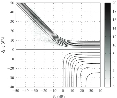
This is illustrated for the stop “t” inFigure 12. In the same manner the detection counts and the missed detections are illustrated in Figures13and14, respectively.
It can be concluded fromFigure 12that under the given measurement conditions during the closure of the stop “t” the SNR ξ1 is roughly −30 dB and the SNR rise during
the burst is around 40 dB. If the SNR increase leads to an SNR close to or less than 0 dB the stop cannot be detected (Figure 14). In this case a multichannel spatial preprocessing (e.g. [22]) can help to improve the SNR prior to the detection.
Stop “t” whose (ξ1,ξ1→2)-coordinates correspond to a
small LR value can be robustly detected (Figure 13). The histogram thus confirms the theoretical considerations of the preceding subsections.
The experiment could be repeated for a higher or a lower input noise level. This would make the histograms shift towards lower, respectively, higher SNRξ1, so that fewer,
respectively, more phonemes would be detected.
k ax
m pcl
p l
eh kcl
k s
ix tcl
t iy
ah v
kcl k
em pcl
p l
iy tcl
m aa
r kcl
k ix
dx iy
ng pcl
p l
ae nx
iy ng
h#
0 0.2
Distur
bed
speec
h,
y
(
i
)
λ=0.25
0.2 0.4 0.6 0.8 1 1.2 1.4 1.6 1.8 2 2.2 2.4 Time (s)
0 0.25 0.5 0.75 1
LR
Figure11: Example usage of the detector for low-delay detection of instationarities in continuously spoken disturbed speech (bottom, “complexity of complete marketing planning”, [21]). The LR values are plotted on top, the decision thresholdλ=0.25 is represented by the dash-dotted line.
−40
−30
−20
−10 0 10 20 30 40 50
ξ1→
2
(dB)
−50 −40 −30 −20 −10 0 10 20 30 40
ξ1(dB)
0 2 4 6 8 10 12 14 16 18 20
Figure12: Occurrences of phoneme “t” in sentences disturbed at 10 dB mean segmental SNR.
4. Modifications to the Noise Reduction System
With the ability of detecting instationarities in disturbed speech the classical noise reduction system is extended as illustrated in Figure 15. The detection of instationarities is based on the highpass-filtered input signal, y(i). As many noise types show a lowpass characteristic, highpass filtering improves the SNR prior to the detection and hence helps to improve the detection rate. Given the likelihood ratio, LR, at the output of the detector, in the following paragraphs we discuss three possible measures that can be applied on their own or in combination.
In short we propose to
(i) switch the analysis (and synthesis) window of the spectral analysis system for a better temporal resolu-tion during transiresolu-tional segments;
(ii) adapt the decision-directedestimator for the a priori
SNR [12] to allow for a faster and more precise tracking of thea prioriSNR during transitions;
−40
−30
−20
−10 0 10 20 30 40 50
ξ1→
2
(dB)
−50 −40 −30 −20 −10 0 10 20 30 40
ξ1(dB)
0 2 4 6 8 10 12 14 16 18 20
Figure13: Detected occurrences of phoneme “t” (λ=0.1).
(iii) amplify a segment that has been classified as transi-tional to improve speech intelligibility [14,15].
4.1. Window Switching. Figure 16 illustrates how the
non-stationarity detection is applied to the spectral analysis-synthesis window sets presented inSection 2. Block 2 has a length of K2 = 32 samples (2 ms), centered on the short
analysis window, hI(i). Block 1 is initially also of length K1=32 samples but is growing byRsamples per frame shift
as long as no nonstationarity is detected and a maximum length of 5Rsamples is not exceeded. As argued before, this strategy reduces effectively the variance of the LR estimate. If a nonstationarity is detected, block 1 is reset to the last
K1=32 samples.
−40
−30
−20
−10 0 10 20 30 40 50
ξ1→
2
(dB)
−50 −40 −30 −20 −10 0 10 20 30 40
ξ1(dB)
0 2 4 6 8 10 12 14 16 18 20
Figure14: Missed detections of phoneme “t” (λ=0.1).
and an estimate which is built from the speech spectrum estimated in the preceding frame,Sk(m−1):
ξk(m)=α
Sk(m−1)2
σN2(m−1)
+ (1−α)max
|Yk(m)|2 σN2(m)
−1, 0
,
α∈[0, 1[.
(19)
The first estimateξk(m) after a speech onset is ruled by the a posteriori SNR, |Yk(m)|2
/σN2(m), in the second term in
(19) since the feedback term|Sk(m−1)|2/σN2(m−1) is small
due to the speech pause in the preceding frame. Since the second term in (19) is weighted with 1−α, which is typically of the order of −12 dB to −17 dB (α = 0.94 : 0.98), the
a prioriSNR estimate considerably underestimates the true
a prioriSNR during speech onsets [24]. As a consequence, stops, which are normally of low intensity, are often severely attenuated by noise reduction filters based on the decision-directedapproach.
By lowering the parameterα, the response time on fast changes of the SNR can be improved, however, only at the price of an increased distortion of the residual noise (musical noise). Therefore it was proposed to make the parameterαof thedecision-directedapproach time-dependent [25] or time-and frequency-dependent [26]. In [27] the response time of thea prioriSNR estimator on SNR increases is improved with a recursion step in which per frame advance a preestimate of the clean speech spectrum is computed which is then used to determine thedecision-directedestimate of thea prioriSNR.
While in [25, 26] the parameter α is modified frame-by-frame, we propose to change it only if a speech onset is detected. Whenever a significant power increase is reliably detected (LR less than a threshold, LRthresh1), αk(m) is
reduced for those frequency bins k where speech activity is likely. The latter is important, as broadband reduction ofαk(m) leads to audible musical noise in those frequency bands that are not masked by the speech.
To realize the desired behavior ofαk(m) the maximum likelihood estimate of the a prioriSNR is smoothed along frequency and is then linearly mapped to the range of values of α ∈ [0,αmax] where αmax < 1 is typically 0.94 : 0.98.
Estimates of the a priori SNR greater or equal to 15 dB very likely indicate the presence of speech and are therefore mapped toαk(m) = 0 to preserve the speech presence in those frequency bins. Estimates less or equal to 0 dB are very likely dominated by noise and are therefore mapped to
αk(m)=αmax.
This procedure is applied for three consecutive frames after the onset detection. After this time the feedback of the estimated clean speech spectra Sk(m−1) in (19) will have established more robust estimates,ξk(m), so thatαk(m) can be increased again toαmax until the next onset will be
detected.
4.3. Amplification of Transients. In [13] the effect of adjusting the consonant-vowel intensity ratio on consonant recog-nition by hearing impaired subjects was investigated. The recognition of stops was significantly improved when the release burst of the stop was amplified. The improvement reached a maximum when the consonant-vowel intensity ratio was amplified by roughly 8 to 14 dB (depending on the stop, the vowel environment, audiogram configuration, etc.). While the results of this study relate to the undisturbed case, in [14] speech material was used that was disturbed to 6 dB SNR with a 12-talker babble. The effects of three modifications are compared: (1) increasing the duration of consonants, ( 2) increasing the consonant-vowel intensity ratio by 10 dB, and ( 3) a combination of (1) and (2).The most significant improvements are obtained from increasing the consonant-vowel intensity ratio. Similar results are obtained in [15] where bursts of plosives are amplified by 12 dB. As apposed to the studies presented before, in [15] also sentence material was used as stimulus. In this case less improvements from the amplification of the consonantal region were observed compared to the case where consonant-vowel-consonant stimuli were used. The clean speech was disturbed with speech-shaped noise at−5, 0 and 5 dB SNR.
Based on these findings, in our proposed system, in addition to the window switching, we amplify the samples of those frames that most probably contain a speech onset. To this end, the frame data is amplified with a gain Gtrans,
whenever the LR (13) falls below a threshold LRthresh2. In
the cited works, the point in time and the duration of a consonant is perfectly known as annotated speech was used in the investigations. In our case, speech onsets have to be detected in the disturbed signal. To account for the uncertainty of the detection we let the gain linearly increase with increasing reliability of the nonstationarity-decision, that is the smaller the values ofLRthe higher is Gtrans, cf.
Figure 17. As soon as the LR exceeds the threshold LRthresh2,
we let the gain Gtrans decay exponentially to Gtrans = 1
FFT IFFT
HP
Index of window set under use
LR Analysis window switching
Estimation of clean speech
Non-stationarity
detection
Synthesis window and overlap-add y(i)
K K
s(i)
Figure15: Overview of a noise reduction system with nonstationarity detection. The stationarity decision controls the choice of the spectral analysis-synthesis window and the estimation of the clean speech spectral coefficients.
Time
R
2M K1K2
Figure16: Stationarity detection applied to the analysis system with frame advance R and short windows of length 2M = 4R. In the example, the analysis window is switched from long asymmetric to short symmetric. Block 2 consists ofK2 =Rsamples. Block 1
has initially lengthK1 =K2but grows byRsamples as long as no
nonstationarity is detected and until an upper limit for the length is reached.
LR
0 LRknee 1
0 1
Gmaxtrans Gtrans
Figure17: Mapping the likelihood ratio LR to a frame amplifica-tionGtrans.
speech. A limitation of the maximum gain to 3.5 dB results in a clearly perceptible amplification of transient sounds like bursts of stops, but preserves the naturalness of the speech. It is important to notice that the proposed increase of the consonant-vowel intensity ratio becomes feasible only with short analysis windows. The amplification of the data captured under a classical long analysis window can produce audible noise prior to the amplified speech onset if the onset occurs only in the most recent samples of the frame. With the concept of switched windows, however, the short analysis
and synthesis windows will be used whenever a speech onset is detected, hence preventing audible prenoise.
5. Results
5.1. Example of Estimated Speech. To illustrate the con-sequences of the measures proposed in Section 4, speech disturbed with speech-shaped noise has been denoised using a frequency domain Wiener filter anddecision-directed esti-mation of thea prioriSNR. The spectral analysis is realized using either permanently the asymmetric long window,
hII(i), or the short and long analysis window set,hI(i),hII(i),
switched according to the nonstationarity decisions taken by the detector presented inSection 3. In another case, not only the window set is switched, but also the parameterαof the
decision-directedapproach is modified as proposed in4.2. Time-domain signals of the utterance “Poach the apples in. . .” are given inFigure 18.Figure 18(a)shows the clean and the noisy signal at 10 dB SNR (speech-shaped stationary noise).Figure 18(b)contains the output of a Wiener filter single-channel noise reduction. Since only the long spectral analysis window is used, the stops at 0.05 seconds or at 0.75 seconds are considerably distorted. InFigure 18(c)the result obtained with a signal dependent switching between long and short analysis windows is shown. At the bottom, the window decision is plotted. By using the short analysis window during transient sounds the distortion of these sounds in the filtered output can be reduced. Finally, in
Figure 18(d)the result with additionally modified decision-directedapproach is plotted. It shows considerable improve-ments of the transients. In particular the two stops at 0.05 s and at 0.75 s are very well preserved in the filtered output.
−0.04
−0.02 0 0.02 0.04 0.06
0 0.2 0.4 0.6 0.8 1
Time (s)
Noisy
Clean
(a) Clean and noisy speech (“Poach the apples in. . .”) at 10 dB SNR, speech-shaped stationary noise.
−0.04
−0.02 0 0.02 0.04 0.06
0 0.2 0.4 0.6 0.8 1
Time (s)
(b) Filter output using only the long window set (hII(i), fII(i)).
−0.04
−0.02 0 0.02 0.04 0.06
0 0.2 0.4 0.6 0.8 1
Time (s)
Short Long
(c) Filter output using either short or long window set, switched according to the window decision plotted at the bottom.
−0.04
−0.02 0 0.02 0.04 0.06
0 0.2 0.4 0.6 0.8 1
Time (s)
Short Long
(d) As before, but additionally with modifieddecision-directedapproach.
Figure18: Time-domain signals of input and the results obtained after noise reduction with Wiener filter and the methods proposed in Sections4.1and4.2.
10 20 30 40 50 60
F
req
uency
b
in
50 100 150 200 250 300 350 400 450 Frame indexm
−60
−40
−20 0
(a) Clean speech (“Poach the apples in. . .”).
10 20 30 40 50 60
F
req
uency
b
in
50 100 150 200 250 300 350 400 450 Frame indexm
−60
−40
−20 0
(b) Speech plus speech-shaped noise at 10 dB SNR.
10 20 30 40 50 60
F
req
uency
b
in
50 100 150 200 250 300 350 400 450 Frame indexm
−60
−40
−20 0
(c) Filter output using only the long window set (hII(i), fII(i)).
10 20 30 40 50 60
F
req
uency
b
in
50 100 150 200 250 300 350 400 450 Frame indexm
−60
−40
−20 0
(d) Filter output using either short or long window set, switched according to the window decision plotted at the top (high level means short window set (I) is used, else long window set (II)).
10 20 30 40 50 60
F
req
uency
b
in
50 100 150 200 250 300 350 400 450 Frame indexm
−60
−40
−20 0
(e) As before, but additionally with modified decision-directed ap-proach.
−90
−80
−70
−60
−50
−40
−30
−20
(dB)
10 20 30 40 50 60
Frequency bin,k Sk(m)
Yk(m)
Sk(m), analysis window:hII(i) only
Sk(m), analysis windows:hI(i),hII(i) switched
Sk(m), analysis windows:hI(i),hII(i) switched and modifieddecision-dir.approach
Figure20: Spectra of clean,Sk(m), noisy (speech-shaped additive noise),Yk(m), and estimated clean speech,Sk(m) of the phoneme [p] in “poach.” The estimated clean speech is obtained by Wiener filtering using a spectral analysis based on either the asymmetric long window only,hII(i), or based on the window sethI(i) and hII(i) fromFigure 1. If the window set is used the window decision is based on the nonstationarity decision. The thin solid black line shows the result if additionally to the switched window set the proposed modification of thedecision-directedapproach is applied. Frame amplification (cf.4.3) is not shown here. The above spectra have been created using a 128-point DFT and Hann windowed data (sampling frequency fs=16 kHz).
−0.2 0 0.2 0.4 0.6 0.8 1 1.2
R
elati
ve
fr
equency
−8 −6 −4 −2 0 2
Difference of log-spectral distortion
hII(i) only
hI(i),hII(i), switched
hI(i),hII(i), swit. and mod.decision-dir.app.
Figure21: Relative frequencies of the improvements of log-spectral distortion in 2792 occurrences of the phoneme [d]. Values less than zero signify less distortion of the proposed system as compared to a system using a square-root Hann window for spectral analysis-synthesis that produces the same small system delay.
In Figure 20 we show sample spectra of the denoised speech during articulation of the phoneme [p] in the word “poach.” For comparison, the spectra of the clean speech,
Sk(m) (thick solid green line), and of the noisy observation,
Yk(m) (dotted black line), are also plotted.
At frequency bins k = 22. . .30 and k = 40. . .50 the speech spectrum is better preserved when using the switched window set (dashed blue line) as compared to the results obtained with the long asymmetric window only (red solid line). The maximum gain observed in this example is about 4 dB. If additionally the proposed modification of thedecision-directedestimator of thea prioriSNR is realized (thin solid black line), the estimated speech spectrum, on average, much better preserves the actual speech spectrum. As a consequence, the phoneme sounds sharper than without modification of the decision-directed SNR estimator and without window switching.
5.2. Instrumental Evaluation. In our experiment 4132 clean speech utterances [21] disturbed with additive speech-shaped noise at 10 dB SNR have been processed with a Wiener filter single-channel noise reduction using either square-root Hann windows (length 8 ms) for spectral analy-sis and syntheanaly-sis or the proposed system. In terms of delay the square-root Hann window is comparable with the proposed system (cf.Table 1, A versus B). Then, for every occurrence of a phoneme the intelligibility-weighted [28] mean log-spectral distortions has been determined [29]. The mean is computed over frames with a segmental SNR greater than 5 dB. A measurement frame is only 2 ms long in order to be able to resolve the short bursts of stops. Finally, the differences between the spectral distortion produced by the proposed system and the distortion produced by the square-root Hann windows was determined. Figure 21 shows the histogram of the differences for the example of the phoneme [d]. A negative value signifies that the distortion obtained with the proposed system is less than in case of the square-root Hann windows. Below the histograms the mean and the 5%- and 95%-significance levels of the three distributions are indicated. Using the long window without switching to the short window (thick solid red line) produces on average a similar distortion as obtained with the reference window. We observe slightly less distortion when the window is switched to the short window (thick blue dashed line). When additionally thedecision-directedapproach is modified (thin solid black line) the average distortion considerably reduces (about 2.8 dB less than the reference). The distribution becomes bimodal because not all occurring phonemes [d] are detected.
5.3. Listening Tests. Informal experiments conducted with four expert listeners confirmed the improved reproduction of stops with the proposed modification of the noise reduc-tion system. Stareduc-tionary speech-shaped noise and cafteria-babble was used at 5 and 10 dB SNR. The amplification
Gtrans of transient frames (see Section 4.3) was limited to Gmax
trans = 3.5 dB because this resulted in natural sounding
speech. Note that in [13–15] stronger amplifications of about 10 dB are proposed to achieve a higher speech intelligibility.