Time-Scale and Time-Frequency Analyses of Irregularly
Sampled Astronomical Time Series
C. Thiebaut
Centre d’Etude Spatiale des Rayonnements, 9 avenue du Colonel Roche - Boite postale 4346, 31028 Toulouse Cedex 4, France Email:[email protected]
S. Roques
Laboratoire d’Astrophysique de l’Observatoire Midi-Pyr´en´ees, 14 avenue Edouard Belin, 31400 Toulouse, France Email:[email protected]
Received 27 May 2004; Revised 21 January 2005
We evaluate the quality of spectral restoration in the case of irregular sampled signals in astronomy. We study in details a time-scale method leading to a global wavelet spectrum comparable to the Fourier period, and a time-frequency matching pursuit allowing us to identify the frequencies and to control the error propagation. In both cases, the signals are first resampled with a
linear interpolation. Both results are compared with those obtained using Lomb’s periodogram and using the weighted wavelet
Z-transformdeveloped in astronomy for unevenly sampled variable stars observations. These approaches are applied to simulations and to light variations of four variable stars. This leads to the conclusion that the matching pursuit is more efficient for recovering the spectral contents of a pulsating star, even with a preliminary resampling. In particular, the results are almost independent of the quality of the initial irregular sampling.
Keywords and phrases:astronomical time series, irregular sampling, time-scale methods, time-frequency methods, wavelets, matching pursuit.
1. INTRODUCTION
Nonuniform sampling problems arise in many astronomi-cal fields [3,22], particularly in Stellar physics when one ob-serves the light curves of variable stars (asteroseismology) or spectroscopic variabilities. The frequencies deduced from the light variations of such stars represent an important source of information. In particular, they can help constrain stel-lar evolution models, because the structure of the vibration modes and their frequency separations may yield physical parameters of the star, such as the rotation period or the composition of its layers [1,16]. Another field of applica-tion concerns the development of automatic classifiers for variable stars, where the period is a very discriminating pa-rameter [27]. Of course, observations have to cover a long enough time span for the best possible resolution of the power density spectra. The difficulty in obtaining such com-plete observations is well known: the lack of information is essentially due to diurnal cuts, poor weather conditions, or equipment malfunctions. Generally, such astronomical data
This is an open access article distributed under the Creative Commons Attribution License, which permits unrestricted use, distribution, and reproduction in any medium, provided the original work is properly cited.
are of two types. First, evenly spaced time series separated by wide gaps [9] (typically day/night alternation for observa-tions of short-period stars taken over several days). In that case, many different methods have been proposed to deal with this problem, for example, autoregressive models which predict data for the gaps [21] combined with observing cam-paigns with telescopes at several different longitudes [18]. Second, unequally spaced time series with samples missing almost everywhere. Here, data under study are from sev-eral years of observations (long-period stars) with a mean sampling rate of a few days (here, telescope failures or bad weather conditions are the main causes of the gaps [4]). This second case is considered in this paper. Of course, problems of this kind do not arise only when processing astronomical signals. In an astrophysical context, it is of capital importance to solve them in order to carry out a physical interpretation of the observations, no other experimental alternative is pos-sible.
In this context, wavelet analysis [6] and time-frequency anal-ysis [10], which have the ability to decompose the signal into contributions localized both in time and in scale (or fre-quency), are thus especially attractive to obtain this informa-tion. These analyses are widely described for simulated data for example in Szatm´ary et al. [26] and in variable star re-search in Kiss and Szatm´ary [14]. These authors conclude that such methods of decomposition, labeled with a scale and a position parameter, provide interpretable visual represen-tations of astronomical data, as an alternative to the standard spectral analysis.
Unfortunately, wavelet and time-frequency analyses are generally not directly applicable to the particular case of ir-regularly sampled data [24], thus one often uses standard techniques like periodograms [13]. However, with such a simple spectral technique, intervals including low-amplitude peaks are hard to identify in the processed data because each feature is contaminated by noise and convolved by a function whose nature closely depends on the irregular distribution of the data. As the corresponding aliases can be of substantial amplitude, they can lead to the confusion of features due to real oscillations with those arising from the segmented na-ture of the observing window. If one deals only with signals whose spectra are dominated by a small number of compo-nents at discrete frequencies, nonlinear deconvolution meth-ods like the widely used CLEAN technique are efficient [20]. Obviously, in the absence of any a priori information on the spectrum to be recovered, the case considered here, this tech-nique becomes unreliable.
Time-frequency methods are efficient, particularly when an examination by eye of the periodogram leads to a failure (seeSection 4). If data sampling is not equidistant, one must first resample the signal to build a regular sampling, before applying a time-frequency method. Several techniques exist to do this and the associate errors are widely discussed in the literature. de Waele and Broersen [8] divide them into simple and complex methods. In particular, they conclude that linear interpolation is a robust resampling method al-though it provides a signal whose standard deviation is bi-ased with a systematic error. However, this error can be cor-rected by replacing the standard deviation obtained with lin-ear interpolation by the value given with the method they propose: the nearest neighbor resampling. Foster [11] pro-posed a rescaled wavelet technique called weighted wavelet
Z-transform(WWZ). It is developed specifically for unevenly sampled data in the context of observation of variable stars: here, the wavelet is rescaled to satisfy admissibility condi-tion on such irregular sampling. One can for example read the paper of Haubold [12] for an interesting analysis of this method. In this paper, our results will also be compared with those obtained by the WWZ technique.
The signals under consideration in this paper being ir-regularly sampled, we have opted for a processing method in two stages: (1) we have resampled the data by using a linear interpolation (with a sampling rate typically equal to one day and without applying any additional smooth-ing or filtersmooth-ing—contrary to preprocesssmooth-ing techniques rec-ommended by Buchler et al. [2]), (2) we have then applied
two appreciably different types of time-frequency analyses: a global wavelet transform and the associated wavelet spec-trum [28], which is described in Section 2, and a match-ing pursuit decomposition [17] developed in Section 3. The results are discussed and compared (Section 4) to those found using a periodogram and WWZ, for simu-lated signals and for light curves of four variable stars: T Camelopardis—a Mira variable star of period 373.2 days, S Persei—a Type C semiregular star of period 822 days, AC Herculis—a Type A RV Tauri variable star of period 75.01 days, and RV Tauri—a Type B RV Tauri star of pe-riod 78.73 days. These periods are those specified in the fourth edition of the General Catalog of Variable Stars, see
http://www.sai.msu.su/groups/cluster/gcvs/gcvs. This leads us in particular to forecast a chaotic light curve of AC Her-culis as predicted by Kollath et al. [15].
2. GLOBAL WAVELET SPECTRA
We recall that a wavelet decomposition is an expansion of an arbitrary function into smoothed localized contributions la-beled by a scale and a time parameter. Its aim is to expand a signal into a series of coefficients of specified energy and then to capture fine and coarse features at different scales. More-over, it provides an easily interpretable visual representation of the signal (see, e.g., the book of Daubechies [6] for more details). Wavelets are generated by a functionψ(t) namedthe analyzing wavelet. This function should have a finite energy, and its integral should vanish. These two conditions mean that the wavelet should oscillate like a short wave. The ana-lyzing wavelet isthe motherof the wavelet family. The wavelet family{ψ}is generated by translating and dilating the ana-lyzing wavelet. Then, one can write any function as a linear combination of the elements of the family.
Here we consider the continuous wavelet transform of a real signals(t) with respect to the analyzing waveletψ(t). The wavelet transform is defined as the function
C(b,a)=√1 a
ψ∗
t−b
a
s(t)dt (1)
on the time-scale plane. Here,a is a dilation scale andba translation parameter; the asterisk denotes the complex con-jugate. The qualitative information given by the visual output supplements the information obtained by inspection of the signal itself, or its Fourier transform. The wavelet transform displays information in a wide range of scale parameters on a single picture.
The choice of the analyzing wavelet is generally guided by a compromise between time and frequency resolutions and by its ability to capture localized features of the signal. As we are essentially interested in wavelet power spectra, the wavelet we used here is the Morlet wavelet (a complex expo-nential modulated by a Gaussian)
ψ0(t)=π−1/4exp
iω0t
exp
−t2
2
which offers high frequency resolution because it is very well localized in frequencies. In contrary, using derivative of Gaussian wavelet would result in a good time localization, but a poor one in frequency.
The global wavelet transform used in our analysis corre-sponds to a continuous wavelet approach allowing the defi-nition of a global wavelet spectrum as the square of the mod-ulus of the wavelet coefficients for each scale together with statistical significance tests [28]. The aim of the method pro-posed by these authors is to provide quantitative tools asso-ciated with wavelet analysis. This leads in particular to an equivalent Fourier period(which can be derived analytically for each wavelet function) which can be easily compared to the Fourier power spectrum or to the periodogram.
3. MATCHING PURSUIT ALGORITHM
The matching pursuit algorithm, introduced by Mallat and Zhang [17], allows us to choose, in a given redundant finite dictionary of time-frequency waveforms, a set of vectors that match the signal as well as possible. The dictionaryDis de-fined as a family (not a basis) of time-frequency functions obtained by dilating, modulating, and translating a single real even function k(t) ∈ L2(R). Theatoms(elements) of the dictionary are defined by
kν(t)=√1
ak
t−b a
eiωt, (3)
whereais the dilation scale,bthe translation parameter, and
ωa frequency modulation. One definesν= (a,b,ω) as the atom index in the dictionary. Note that the factor 1/√a nor-malizes theL2(R) norm ofk
ν(t) to unity. If the windowk(t) is Gaussian, the joint time-frequency localization of all the atoms is a minimum, and in this casekν(t) is aGabor
func-tion. Note that the family{kν}is not a wavelet family in the sense that a given dilation allows several analyzing frequency values. It can be seen as a superposition of a wavelet trans-form and a short-term Fourier transtrans-form. In particular, the underlying family is nonorthogonal. In practice, the atoms of the family are thus oscillating functions modulated by win-dow functions. They are generated by two mother functions that satisfy localization properties: a window function k(t) (a “Spline 0” in this paper—seeFigure 1) and a wavelet-like function. For each value of the atom indexν, one has a new atom of the family, until obtaining a complete collection of atomic waveforms.
A matching pursuit algorithm computes adaptive sig-nal representations: it expands any sigsig-nal into a set of atoms selected among the redundant dictionaryD, to match its components as well as possible, through iterated one-dimensional projections.
In our particular case, it is the resampled light curves(t), from which the mean value has been subtracted after resam-pling so that it becomes zero mean, which is approximated by a single vectorkν1chosen from the dictionaryDsuch that
|s(t),kν1(t)|is as large as possible. Here,·,·denotes the
10 20 30 40 50 60 70 80 90
Number of atoms 10
Er
ro
r
(%)
Gaussian Hamming Hanning Blackman
Spline 0 Spline 1 Spline 2 Spline 3
Figure 1: Reconstruction error versus number of atoms of the matching pursuit decomposition for each shape of the even real
functionk(t) (in logarithmic scale).
scalar product inR. In practice, one has to compute a scalar product for all the values ofν. The vectorkνgiving the largest one iskν1.
The light curve is then decomposed into the form
s(t)=s(t),kν1(t)
kν1(t) +Rs(t), (4)
whereRs(t) is the residual vector after approximatings(t) in the “direction”kν1(t). Clearly,kν1(t) is orthogonal toRs(t), and hence, one has the relation
s(t)2
= s(t),kν1(t) 2
+Rs(t)2, (5)
where · denotes the Euclidian norm. Note that if the fam-ily{kν}is nonorthogonal, the vectorkν1(t) is orthogonal to the residualRs(t). This important property allows the con-struction of the algorithm: the main idea of the matching pursuit is to subdecompose the residue Rs(t), by finding a vectorkν2(t) that matches it as well as possible, as was done fors(t). Each time, the procedure is repeated on the obtained residue:
s(t)=s(t),kν1(t)
kν1(t) +Rs(t),
Rs(t)=Rs(t),kν2(t)
kν2(t) +R 2
s(t), ..
.
Rns(t)=Rns(t),kνn(t)kνn(t) +Rn+1s(t).
(6)
Finally, the signal is decomposed into
s(t)= ∞
i=1
Ris(t),k
νi(t)kνi(t), (7)
where the atoms kνi(t) are the ones that match the signal structures as well as possible. We can then build a hierarchy of the main signal structures (kν1(t),kν2(t),. . .,kνn(t)) yield-ing a time-frequency energy distribution.
An energy conservation theorem results from (5):
s(t)2
= ∞
i=1
Ris(t),k
νi(t) 2. (8)
The energy density ofs(t) in the time-frequency plane (t,u) is defined by
(Es)(t,u)= ∞
i=1
Ris(t),k
νi(t) 2Wkνi(t,u), (9)
where (Wkνi)(t,u) is the Wigner-Ville distribution [29] de-fined as follows:
Wkν(t,u)=
∞
−∞kν
t+τ 2
kν∗
t−τ
2
e−iuτdτ. (10)
In practice, it is this energy densityEs(9) that is represented in the time-frequency diagrams. Note that this density does not include the interference terms of the Wigner-Ville distri-butions, because it is computed from an atomic decomposi-tion ofs(t).
Decomposition onto orthonormal basis or the method of Coifman and Wickerhauser [5] selects in a global way the ba-sis that is best adapted to the signal properties. The results as-sociated with these methods are hardly interpretable. On the contrary, the matching pursuit decomposition is a construc-tive process which allows to detect and characterize the time-frequency components one by one, from the highest energet-ics one to the lowest.
In a matching pursuit diagram, we can choose to select only some atoms representing the structures of interest. In our case, these are the most coherent ones. The correspond-ing atoms appear as long (in time) elements in the time-frequency plane (horizontal atoms). As the noise of the time series does not correlate well with any long lifetime dictio-nary element, its information is diluted and then subdecom-posed in several “stains” localized in a short time interval. The peaks, even of large amplitude, which do not correspond to star oscillations but are artifacts due to the sampling or to the gaps of the observing window or corresponding to highly transient phenomena appear in the time-frequency diagram localized in a very short time period, in a large fre-quency range (vertical atoms). A simple operation, keeping only the long lifetime atoms (whatever their frequency), al-lows us to eliminate spurious information (e.g., correspond-ing to noise).
The shape of the even real functionk(t) can be chosen according to various criteria, while still in agreement with the mathematical conditions authorizing the matching pur-suit decomposition. These criteria depend on the adaptabil-ity of k(t) to the studied signal and on some oversensitiv-ity to errors. Eight different window shapes have been con-sidered: Gaussian, Hamming, Hanning, Blackman, Spline 0, Spline 1, Spline 2, and Spline 3. Their description can be found in Oppenheim and Schafer [19] and in de Boor [7].
Figure 1presents the evolution of the quadratic reconstruc-tion error versus the number of atoms used to decompose a simulated signal with these eight different windows. The tested signal is a regularly spaced 1200-point-long signal, the sum of two cosines with periods of 33.3 and 100 days. The quadratic reconstruction error is defined as the norm of the residual signal between the simulated and the reconstructed ones divided by the norm of the simulated signal. The Black-man window always gives the largest error. The Gaussian and Spline 3 windows also show large errors whatever the num-ber of atoms. Up to 50 atoms, the Spline 0 window is clearly the best. For a decomposition with more than 50 atoms, all the windows, except the Blackman window, present similar reconstruction errors. Following this, as the signals we ana-lyze here are of quite constant amplitude, the adaptation of
k(t) to the data leads us to choose the Spline 0 window. In-deed, the rectangular shape of this window does not create an amplitude modulation.
4. APPLICATION EXAMPLES AND THE COMPARISON WITH THE PERIODOGRAM AND WITH THE WWZ
Although we have analyzed the light curves of four stars, we focus on only two of them (AC Herculis and RV Tauri—see
http://www.kusastro.kyoto-u.ac.jp/vsnet/index.html) and the results are summarized inTable 1.
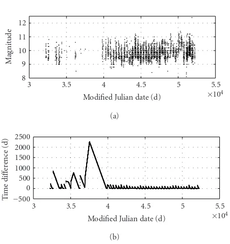
The data set of the irregularly sampled observations spans JD 2 440 000–2 450 000 for AC Herculis and JD 2 432 223–2 452 270 for RV Tauri (seeFigure 2a). JD is the Julian day number, number of days that have elapsed since noon of January 1, 4713 B.C. of our civil calendar. In addition, we have created two artificial signals (sum of two cosines with periods of 100 and 33.3 days) with the same nonequidistant sampling scheme as those of AC Herculis and RV Tauri, and without added noise. The choice not to add noise is linked to the concern of analyzing only the effect of the nonuniform sampling and how the methods address this question.
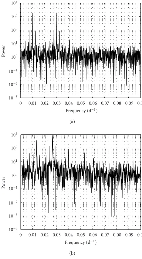
The periodograms from these variable star observations and those from the simulated signals made from the same ir-regular sampling are presented in Figures 3and4. In these figures (top), the two 100-day and 33.3-day periods are vis-ible. The clearly identifiable aliases essentially correspond to the annual cycle of the observations, proving that one finds it effective in the sampling.
Table1: Results for the four variable stars (column 1). The sampling quality is defined by the mean number of observations per day (column 2). The reconstruction error computed for the matching pursuit analysis is presented (column 3). The known period and those found with
the different analyses are indicated (columns 4–8): periodogram (PPerio), GWS (PGWS), matching pursuit decomposition (PMP), and weighted
waveletZ-transform (PWWZ). In the WWZ,c=0.005 for data of S Per. and T Cam.,c=0.04 for AC Her, andc=0.0125 for RV Tau. In
brackets: double periods are also found and are corresponding to the periods indicated in the fourth edition of the General Catalog of Variable Stars.
Star O/day Error PGCVS PPerio PGWS PMP PWWZ
AC Her. 0.757 3.71% 75.01 37.74[75.19] 37.00[75.00] 37.73[75.19] 38.24[71.43]
S Per. 0.112 11.22% 822.00 806.40 826.00 819.00 831.90
RV Tau. 0.190 8.53% 78.73 39.26 39.00 39.29[8.77] 38.8
T Cam. 0.051 10.98% 373.20 371.75 373.00 372.30 371.10
3 3.5 4 4.5 5 5.5
8 9 10 11 12
Modified Julian date (d) ×104
M
ag
nitude
(a)
3 3.5 4 4.5 5 5.5
−500 0 500 1000 1500 2000 2500
Modified Julian date (d) ×104
Ti
m
e
d
i
ff
er
enc
e
(d)
(b)
Figure2: RV Tauri sampling signal (modified Julian date=JD-2 400 000.5).
(c=0.0125) for time and frequency grids, we settled onc=
0.04 for time sampling of AC Herculis and keptc=0.0125 for time sampling of RV Tauri as better compromises in the sense that they were the first lowest values for which we ob-tained the target periods. WWZ applied on these test data can reveal peaks at frequencies 100.5 and 33.2 days for time sampling of AC Herculis and at frequencies 100.0 and 32.9 days for time sampling of RV Tauri. The same constants will be used for application to the observations.
In order to perform time-frequency and time-scale anal-yses, the data (simulated and real) have also been linearly in-terpolated with a time step equal to one day. As the known periods of the studied variable stars are more than 50 days, Shannon’s theorem is satisfied. The so-interpolated signals are presented in Figures 5and6(simulated) and Figures7
and8(real). Note that contrary to the case of AC Herculis, whose missing samples are well distributed throughout the observation, RV Tauri data contain very large gaps at the be-ginning of the run.
We then define two “sampling” signals for which each value is equal to the time step of the AC Herculis and RV Tauri data, respectively. Lettibe the time when the data are available. The sampling signal values areti+1−ti(the wider the gap, the larger the value—seeFigure 2b). The “sampling” signals are normalized so that their variances are the same as the corresponding simulated signals. These sampling signals are used in the two following sections: their wavelet trans-forms are compared to those of simulated and real signals.
4.1. Results from the simulations
The wavelet power spectrum (WPS) and the global wavelet spectrum (GWS) obtained for both simulations are pre-sented in Figures 5 and6. The Torrence and Compo [28] approach provides statistical tools for establishing the va-lidity of the results. This allows us to show in the GWS the 95% confidence level that would be obtained for white noise, which is the noise present in periodic variable stars obser-vations as those studied here (the natural assumption of red noise is not adequate here because these data were obtained from different observers). This level (shown by the dashed line) is quasisuperposed on thex-axis (the linear interpola-tion induces errors comparable to white noise). In the WPS, the continuous white line indicates the cone of influence (zone where the edge effects are important). Information outside this cone is not relevant.
From an examination by eye of the WPS from the sim-ulated signal on AC Herculis sampling (Figure 5b), one can identify the two simulated periods at 100.5 and 33.1 days. The corresponding GWS (Figure 5c) shows these two periods which are over the 95% confidence level. In the WPS from the simulated signal from the RV Tauri sampling (Figure 6b), one is also able to identify the two periods also at 100.5 and 33.1 days, although in a more indistinct way, and a third one at 230 days. The large zone due to the bad sampling at the beginning of the run, around t = 36 000 modified Julian days (MJD = JD-2 400 000.5), appears as a large stain in the low frequencies. Although it is inside the cone of influ-ence, it overshadows the presence of both periods. The GWS (Figure 6c) highlights the same problem.
0 0.01 0.02 0.03 0.04 0.05 0.06 0.07 0.08 0.09 0.1 10−3
10−2
10−1
100
101
102
103
104
Frequency (d−1)
Po
w
er
(a)
0 0.01 0.02 0.03 0.04 0.05 0.06 0.07 0.08 0.09 0.1 10−4
10−3
10−2
Frequency (d−1)
10−1
100
101
Po
w
er
102
103
(b)
Figure3: Periodograms from the AC Herculis light curve (b) and from the corresponding simulated signal (a), presented on a loga-rithmic scale.
results of the GWS, if the presence of a peak of significant amplitude can be explained or not by the irregularity of the sampling. In these simple cases, we can verify that the irregu-lar sampling of RV Tauri is responsible for the peaks above roughly 500 days, detected in the GWS (Figure 10). Their nonvalidity was already confirmed by their position outside the cone of influence. However, the GWS from the sampling signal does not explain the 230-day period (see Section 5). Note also that for AC Herculis (Figure 9), the two structures visible at 365 days and 183 days obviously correspond to the annual cycle of the observations.
To complete our analysis, we examine the matching pur-suit decomposition of the same simulations. The results pre-sented here use the free graphical user interface developed at our institute (http://webast.ast.obs-mip.fr/people/fbracher)
0 0.01 0.02 0.03 0.04 0.05 0.06 0.07 0.08 0.09 0.1 10−4
10−3
10−2
10−1
Frequency (d−1)
Po
w
er 100 101
102
103
(a)
0 0.01 0.02 0.03 0.04 0.05 0.06 0.07 0.08 0.09 0.1 10−5
10−4
10−3
10−2
Frequency (d−1)
Po
w
er
10−1
100
101
102
(b)
Figure4: Periodograms from the RV Tauri light curve (b) and from the corresponding simulated signal (a), presented on a logarithmic scale.
based on the LastWave software of Bacry available athttp:// www.cmap.polytechnique.fr/∼bacry/LastWave/.
The linearly interpolated simulated signals are decom-posed into functions from the dictionary Dwith a Spline 0 window. The energy density of the 100 first atoms (kν1(t),kν2(t),. . .,kν100(t)) is shown on Figures11and12. The long atoms represent the most coherent structures of the sig-nal. The peaks which do not correspond to Stellar oscillations but are artifacts due to the sampling appear localized on a short time or cover a large frequency range (vertical atoms).
4.1 4.2 4.3 4.4 4.5 4.6 4.7 4.8 4.9 ×10⁴
−4 −2 0 2 4
Modified Julian date (d)
M
ag
nitude
(a)
4.1 4.2 4.3 4.4 4.5 4.6 4.7 4.8 4.9 ×10⁴
1024 512 256 128 64 32 16 8 4 2
Modified Julian date
Pe
ri
o
d
(d
)
(b)
0 50 100
Power (mag2)
Pe
ri
o
d
(d
)
(c)
Figure5: (a) Simulated signal built from the AC Herculis sampling (light curve). (b) Wavelet power spectrum. The continuous white line indicates the cone of influence. (c) Global wavelet spectrum of the simulated signal with a Morlet wavelet. The 95% confidence level that could be obtained for a white noise is shown by the dashed line.
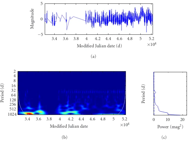
3.4 3.6 3.8 4 4.2 4.4 4.6 4.8 5 5.2 ×10⁴
−4 −2 0 2 4
Modified Julian date (d)
M
ag
nitude
(a)
3.4 3.6 3.8 4 4.2 4.4 4.6 4.8 5 5.2 ×10⁴
1024 512 256 128 64 32 16 8 4 2
Modified Julian date
Pe
ri
o
d
(d
)
(b)
0 50 100 Power (mag2)
Pe
ri
o
d
(d
)
(c)
Figure6: (a) Simulated signal built from the RV Tauri sampling (light curve). (b) Wavelet power spectrum. The continuous white line indicates the cone of influence. (c) Global wavelet spectrum of the simulated signal with a Morlet wavelet. The 95% confidence level that could be obtained for a white noise is shown by the dashed line.
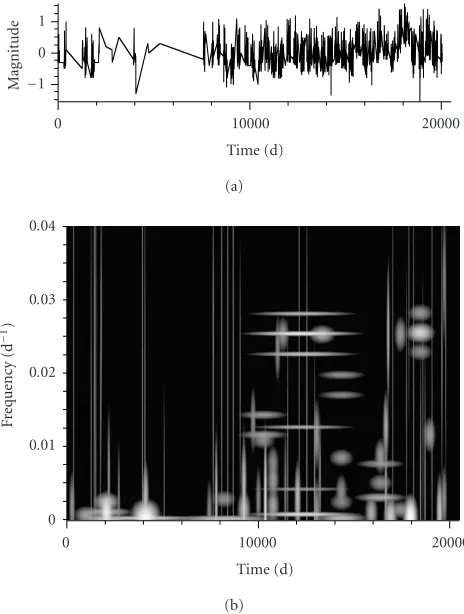
The decomposition of the signal built from the RV Tauri sampling (Figure 12) presents an atom at 0.03 day−1 (with aliases corresponding to the annual cycle) in the second part of the data. Another atom appears at 0.01 day−1 with the same lifetime and aliases. As these atoms
4.1 4.2 4.3 4.4 4.5 4.6 4.7 4.8 4.9 ×10⁴
−5 0 5
Modified Julian date (d)
M
ag
nitude
(a)
4.1 4.2 4.3 4.4 4.5 4.6 4.7 4.8 4.9 ×10⁴
1024 512 256 128 64 32 16 8 4 2
Modified Julian date
Pe
ri
o
d
(d
)
(b)
0 10 20
Power (mag2)
Pe
ri
o
d
(d
)
(c)
Figure7: (a) AC Herculis light curve. (b) Wavelet power spectrum. The continuous white line indicates the cone of influence. (c) Global wavelet spectrum of the simulated signal with a Morlet wavelet. The 95% confidence level that could be obtained for a white noise is shown by the dashed line.
3.4 3.6 3.8 4 4.2 4.4 4.6 4.8 5 5.2 ×10⁴
−5 0 5
Modified Julian date (d)
M
ag
nitude
(a)
3.4 3.6 3.8 4 4.2 4.4 4.6 4.8 5 5.2 ×10⁴
1024 512 256 128 64 32 16 8 4 2
Modified Julian date
Pe
ri
o
d
(d
)
(b)
0 10 20
Power (mag2)
Pe
ri
o
d
(d
)
(c)
Figure8: (a) RV Tauri light curve. (b) Wavelet power spectrum. The continuous white line indicates the cone of influence. (c) Global wavelet spectrum of the simulated signal with a Morlet wavelet. The 95% confidence level that could be obtained for a white noise is shown by the dashed line.
4.2. Application to the observations
The analysis of the AC Herculis and the RV Tauri light curves was conducted with the same methods. AC Her-culis periodogram (Figure 3b) presents four important peaks
2 4 8 16 32 64 128 256 512 1024 0
10 20 30 40 50
Period (d)
Po
w
er
(m
ag
2) 60
70 80 90 100
Figure 9: Global wavelet spectrum of the simulated signal made from the AC Herculis sampling (solid line) compared to the GWS from the corresponding sampling signal (dashed line).
2 4 8 16 32 64 128 256 512 1024 0
50
Period (d)
Po
w
er
(m
ag
2)
100 150 200 250
Figure10: Global wavelet spectrum of the simulated signal made from the RV Tauri sampling (solid line) compared to the GWS from the corresponding sampling signal (dashed line). The solid line with diamonds represents the dashed line multiplied by a factor 10, for clarity.
two frequencies present aliases corresponding to the annual cycle of the observations. The known period of AC Herculis (T0=75.01 days) is correctly identified, although it appears less energetic than the one atT0/2, and its harmonics atT0/3 andT0/4 are also well detected. Finding half the known pe-riod, revealed by the wavelet analysis and the matching pur-suit as well, will be discussed further (Section 4).
The RV Tauri periodogram (Figure 4b) reveals very noisy behavior, but the results indicate a first peak at 0.025471 day−1 (39.26 days), corresponding to roughly half of the known period of this star, and a second one at 0.00082 day−1
0 1000 2000 3000 4000 5000 6000 7000 8000 9000 −2
−1
Time (d) 0
1 2
M
ag
nitude
(a)
0 1000 2000 3000 4000 5000 6000 7000 8000 9000 0
Time (d)
Fre
q
u
en
cy
(d
−
1)
0.01 0.02 0.03 0.04
(b)
Figure11: Time-frequency decomposition (b) of the simulated sig-nal (a) made from the AC Herculis sampling. Each grey level repre-sents the energy density of each atom.
(1219.5 days) which is the known long period of RV Tauri. Both peaks present aliases corresponding to the annual cycle of the observations.
WWZ analysis for AC Herculis reveals a high-amplitude peak at 38.24 days and a less energetic one at 71.43 days. For RV Tauri, one can surprisingly identify the most prominent peak at 1299 days and two others of same amplitude at 502.51 and 38.8 days (as expected). In both cases, the value of the constantcwas chosen as for the simulated signals:c=0.04 for AC Herculis andc=0.0125 for RV Tauri. However, the heuristic choice ofcmakes it difficult to find evidence for ex-act periods. For example, if one chooses a lower or a higher value forc, periods and/or amplitudes appear to be slightly different. It seems that this point is not discussed in the liter-ature.
Figures7and8present the WPS and the GWS from AC Herculis and RV Tauri, respectively, obtained with the same wavelet (Morlet) as for the simulated signals.
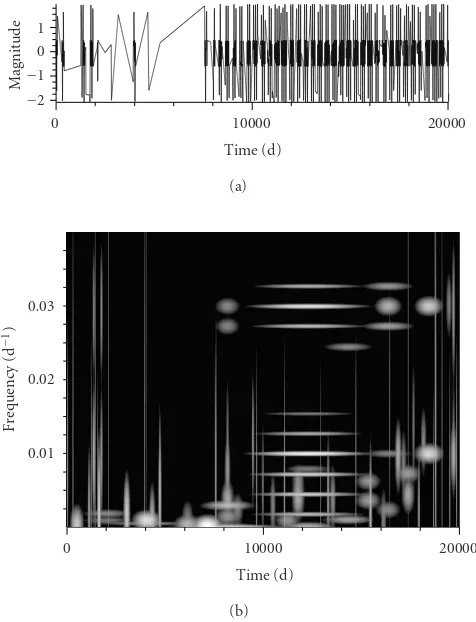
0 10000 20000 −2
−1
Time (d) 0
1
M
ag
nitude
(a)
0 10000 20000
Time (d)
Fre
q
u
en
cy
(d
−
1)
0.01 0.02 0.03
(b)
Figure12: Time-frequency decomposition (b) of the simulated sig-nal (a) made from the RV Tauri sampling. Each grey level represents the energy density of each atom.
harmonics atT0/3 andT0/4 detected in the periodogram do not appear in the WPS. The corresponding GWS is analyzed inFigure 13, superposed on that of the “sampling” signal. In fact, the nature of the sampling explains the last peak (374 days) and even the 141-day one, which are not real.
In the RV Tauri WPS (Figure 8b), only a single period at 39 days in the second part of the time interval can be identi-fied. In the corresponding GWS (Figure 8c), it is also observ-able, together with some others above 500 days, but essen-tially outside the cone of influence. The GWS from RV Tauri is presented in Figure 14. The superposition on that of the corresponding sampling signal explains the peaks above 500 days, due to the sampling, which confirms that they are not real (as was already revealed by the cone of influence).
The matching pursuit analyses of AC Herculis and RV Tauri are computed with a Spline 0 window and keep-ing the first 100 atoms of the decomposition, as was done for the simulated signals (Figures 15and16). Several long lifetime atoms appear in the AC Herculis decomposition: the two most energetic ones are located at the same fre-quency: 0.0265 day−1(37.73 days) and the third oscillates at 0.0133 day−1(75.19 days). AC Herculis known period (75.01 days) is thus well determined, but as in the wavelet analy-sis, half the known period appears first in terms of energy.
2 4 8 16 32 64 128 256 512 1024 0
0.5 1 1.5 2
Period (d)
Po
w
er
(m
ag
−
2)
2.5 3 3.5
Figure13: Global wavelet spectrum of the AC Herculis signal (solid line) compared to the GWS from the corresponding sampling signal (dashed line).
2 4 8 16 32 64 128 256 512 1024 0
2 4 6 8 10 12 14
Period (d)
Po
w
er
(m
ag
−
2)
16 18 20
Figure14: Global wavelet spectrum of the RV Tauri signal (solid line) compared to the GWS from the corresponding sampling signal (dashed line). The solid line with diamonds represents the dashed line multiplied by a factor 20, for clarity.
The harmonics revealed in the periodogram are also present with a high energy in the decomposition (atom 10, fre-quency: 0.0398 day−1 (25.12 days); atom 12, frequency: 0.0531 day−1(18.83 days)).
1000 2000 3000 4000 5000 6000 7000 8000 9000 10000 Time (d)
−1 0 1
M
ag
nitude
(a)
1000 2000 3000 4000 5000 6000 7000 8000 9000 10000 0
0.01 0.02 0.03 0.04
Time (d)
Fre
q
u
en
cy
(d
−
1)
0.05 0.06
(b)
Figure15: Time-frequency decomposition (b) of the AC Herculis signal (a).
Figure 17represents the results of a matching pursuit de-composition of S Persei detailed in another paper [23], show-ing that this type of method can be applied to longer period stars. In that particular case, no long lifetime frequency can be identified by eye in the diagram, but the first atom of the decomposition is at 0.00122 day−1 (819 days) and centered around 10 000 days. This atom is not as long as the strong apparent periodicity in the last part of the data because the energy of a longer lifetime atom (double lifetime) would be smaller (it would take into account the noise on both sides of this part of the light curve). While neither the periodogram nor the wavelet analysis was able to find S Persei known pe-riod (822 days), the matching pursuit analysis offers the pos-sibility of clearly detecting it, since it appears as the first atom of the decomposition.
5. DISCUSSION
Lomb’s periodogram provides well-resolved power density spectra but it is oversensitive to irregular sampling; in some of our cases (e.g., S Persei), the periodogram was too noisy to be analyzed without a preliminary resampling. Moreover, al-though there exists a large literature concerning the statistical properties of the periodogram, its intrinsic nature does not allow us to implement a reconstruction error analysis com-parable to the error provided by matching pursuit analysis.
0 10000 20000
Time (d) −1
0 1
M
ag
nitude
(a)
0 10000 20000
0 0.01
Time (d)
Fre
q
u
en
cy
(d
−
1)
0.02 0.03 0.04
(b)
Figure16: Time-frequency decomposition (b) of the RV Tauri sig-nal (a).
The application of WWZ to the real data leads to the identification of known periods in the four stars. However, in the case of RV Tauri, the prominent period is 1299 days and not 38.8 days as expected. Different choices ofcparameter did not allow us to improve the result. Concerning AC Her-culis, S Persei and T Camelopardis, the most obvious features are consistent oscillations, as they are indicated in the fourth edition of the General Catalog of Variable Stars. We were not able to compute associated errors since, as indicated by Fos-ter [11], their determination is “extraordinary complex.”
The 95% confidence level associated with the WPS and the cone of influence are efficient tools to check if the high-lighted frequencies are meaningful. However, in the regions of interpolated large gaps, neither the cone of influence nor the 95% confidence level is unable to discriminate spurious frequencies. But this method reveals problems for low fre-quencies: in the GWS, high-amplitude peaks are not always explained by those from the sampling signal. The poorest the sampling quality, the more important the problems at low frequencies. These problems are due to the linear interpola-tion, but other interpolation methods (e.g., cubic spline) lead to the same problem. This is what prevents us from carrying out an associated error analysis.
0 10000 −3
−2 −10
Time (d) 1
2 3
M
ag
nitude
(a)
0 10000
0
Time (d)
Fre
q
u
en
cy
(d
−
1)
0.01 0.02
(b)
Figure17: Time-frequency decomposition (b) of the S Persei sig-nal (a).
dominating frequencies of the signal. We can easily define the associated error as the quadratic reconstruction error af-ter decomposition on a large number of atoms (e.g., 400 in our case). Table 1 presents this error for simulated signals (third column) associated with the four variable stars pre-sented in Section 1. The mean number of observations per day is used to estimate the quality of the sampling (second column inTable 1). One can note that the reconstruction er-ror is not correlated with the sampling quality. This is ex-plained by the large choice of atoms of different lifetimes and frequencies offered by the dictionary, which can solve the problem caused by a very incomplete sampling (see, e.g., the error reconstruction for T Camelopardis, compared to its sampling).Table 1also presents the four variable stars peri-ods and the ones found by the periodogram (PPerio), the GWS (PGWS), the matching pursuit decomposition (PMP), and the weighted waveletZ-transform (PWWZ).
We have noted throughout the paper the fact that for AC Herculis, we systematically found half the known period for this star. For RV Tauri, half the known period was also found. However, with the matching pursuit decomposition, we were also able to identify the known period (78.73 days). These two periods also found by Zsoldos [30] are characteristics of the double-wave shape of RV Tauri-like stars.
The matching pursuit decomposition appears to be par-ticularly suitable for a deeper analysis of AC Herculis. In-deed, this star’s light curve is supposed to be chaotic [15]. The matching pursuit analysis is probably the first step to use, towards a simple nonlinear dynamical analysis. Based on certain physical properties of such variable stars, a relevant atom selection allows us to reconstruct a signal characteristic of their structural properties. Note that the WWZ, also high-lighting two periods, would not allow us to select atoms in the same simple manner. Our ongoing work should provide support for the results of Kollath et al. [15]. In the partic-ular case of AC Herculis, our work could also explain why the found period (37.73 days) turns out to be half the pe-riod indicated in the literature (75.01 days) and why these periods are so close from an energetics point of view. In fact, we are probably facing a period-doubling phenomenon: if the star oscillates with a stable fundamental period, say
T0 = 37.73 days, when some parameters vary, a period-doubling bifurcation may occur, leading to another stable pe-riod of 2T0=75.01 days. Both periods can be observed, with a variable amplitude which depends on the run.
6. CONCLUSION
We have used a wavelet analysis and a matching pursuit decomposition to investigate the role of irregular sampling with linear interpolation in the determination of the spec-tral contents of variable star’s light curves and we have com-pared them with results given by a Lomb’s periodogram and by weighted waveletZ-transform (which is a time-scale method that can be compared in its principle to Lomb’s pe-riodogram). The proposed algorithm is composed of two steps: first, a preprocessing is done by interpolating the ir-regularly sampled light curve; second, a scale or a time-frequency analysis is applied on resampled data.
behavior analysis in the continuity of Kiss and Szatm´ary’s work [14].
The known period of AC Herculis at 75.01 days was found (in second position) at 75.19 days by the periodogram and the matching pursuit analysis, at 75.00 days by the GWS and at 71.43 by the WWZ. Harmonics at T0/2,T0/3, and
T0/4 have been clearly identified by the periodogram and the matching pursuit analysis. The two last (resp., three) har-monics do not appear in the GWS (resp., WWZ). The pe-riod of RV Tauri at 78.73 days was not found neither by the periodogram nor by the global wavelet spectrum nor by the weighted waveletZ-transform. However, half of this period could be found at 39.26 days by the periodogram, at 39.00 days by the GWS, and at 38.80 by the WWZ. The matching pursuit decomposition reveals both periods: 39.29 days and 78.77 days. This last method also permits us to conduct an error analysis.
The matching pursuit algorithm thus appears well suited for spectral investigation of irregularly sampled variable stars signals. This study, moreover, offers the new benefit of simply requiring a linear interpolation of the data and allows us to propose a simple guideline for processing such signals:
(1) resample the signal with a linear interpolation; (2) choose a time step compatible with the searched
fre-quency range;
(3) save this new signal as a column ascii file (zero mean); (4) download the matching-pursuit graphical user in-terfaceguimauveat webast.ast.obs-mip.fr/people/fbra-cher(Linux version preferred) and install it with the rpm command;
(5) execute the command guimauve;
(6) open the signal file, set the right time step (menu Sig-nal), decompose the signal (menu Matching), choose the atom number to be investigated (100 by default) and the window (Gaussian by default). Options are ac-tivated by the mouse and the scroll bar;
(7) information on atoms are written at the bottom of the window: ordered in hierarchy, lifetime of the oscilla-tion (“octave” defines the length of the atom as 2octave), time and frequency. The energy is quantitatively acces-sible thanks to the menu File and Save Decomposition. A reconstruction is possible from an atom or parame-ter selection.
Processing a simple linear interpolation before applying a time-frequency analysis offers advantages over a Fourier transform or a periodogram from nonresampled data. How-ever, we plan to investigate, in a forthcoming work, a com-parison of the matching pursuit results with linear interpola-tion of the data versus the interpolainterpola-tion technique proposed by Strohmer [25].
ACKNOWLEDGMENTS
Wavelet Matlab software was provided by C. Torrence and G. Compo, and is available at paos.colorado.edu/research/
wavelets/. The corresponding article [28] is also down-loadable at this URL. Matching pursuit software uses a free graphical user interface developed in our institute and available for Linux (and Windows for a simplest version) athttp://webast.ast.obs-mip.fr/people/fbracher/. The code is based on LastWave software of E. Bacry (http://www.cmap. polytechnique.fr/∼bacry/LastWave/). Weighted wavelet Z -transform was performed using the computer program WWZ developed by the American Association of Vari-able Star Observers (http://www.aavso.org). The authors are grateful to the staffof the Variable Star Network (VSNET) for their online database. The authors wish to thank Herv´e Carfantan and Laurent Koechlin for helpful discussions on early versions of this paper and for their comments and sug-gestions. We gratefully thank Natalie Webb for her essential corrections.
REFERENCES
[1] P. A. Bradley, “Theoretical models for asteroseismology of DA
white dwarf stars,”Astrophysical Journal, vol. 468, pp. 350–
368, 1996.
[2] J. R. Buchler, Z. Kollath, T. Serre, and J. Mattei, “Nonlinear
analysis of the light curve of the variable star R scuti,”
Astro-physical Journal, vol. 462, pp. 489–504, 1996.
[3] M. Carbonell, R. Oliver, and J. L. Ballester, “Power spectra of
gapped time series: a comparison of several methods,”
Astron-omy & Astrophysics, vol. 264, pp. 350–360, 1992.
[4] C. Catala, J.-F. Donati, T. B¨ohm, et al., “Short-term spectro-scopic variability in the pre-main sequence Herbig Ae star AB
Aur during the MUSICOS 96 campaign,”Astronomy &
Astro-physics, vol. 345, pp. 884–904, 1999.
[5] R. R. Coifman and M. V. Wickerhauser, “Entropy-based
algo-rithms for best basis selection,”IEEE Trans. Inform. Theory,
vol. 38, no. 2, pp. 713–718, 1992.
[6] I. Daubechies,Ten Lectures on Wavelets, SIAM, Philadelphia,
Pa, USA, 1992.
[7] C. de Boor,A Practical Guide to Splines, Springer, New York,
NY, USA, 1978.
[8] S. de Waele and P. M. T. Broersen, “Error measures for
resam-pled irregular data,”IEEE Trans. Instrum. Meas., vol. 49, no. 2,
pp. 216–222, 2000.
[9] G. G. Fahlman and T. J. Ulrych, “A new method for estimating
the power spectrum of gapped data,”Monthly Notices of the
Royal Astronomical Society, vol. 199, pp. 53–65, 1982.
[10] P. Flandrin, Time-Frequency/Time-Scale Analysis, Academic
Press, San Diego, Calif, USA, 1998.
[11] G. Foster, “Wavelets for period analysis of unevenly sampled
time series,”Astronomical Journal, vol. 112, no. 4, pp. 1709–
1729, 1996.
[12] H. J. Haubold, “Wavelet analysis of the new solar neutrino
capture rate data for the Homestake experiment,”Astrophysics
and Space Science, vol. 258, no. 1-2, pp. 201–218, 1997. [13] J. H. Horne and S. L. Baliunas, “A prescription for period
anal-ysis of unevenly sampled time series,”Astrophysical Journal,
vol. 302, no. 2, pp. 757–763, 1986.
[14] L. L. Kiss and K. Szatm´ary, “Period-doubling events in the light curve of R Cygni: Evidence for chaotic behaviour,”
Astronomy & Astrophysics, vol. 390, no. 2, pp. 585–596, 2002.
[15] Z. Kollath, J. R. Buchler, T. Serre, and J. Mattei, “Analysis of
the irregular pulsations of AC Herculis,”Astronomy &
[16] D. Koester and G. Chanmugam, “Physics of white dwarf
stars,”Reports on Progress in Physics, vol. 53, no. 7, pp. 837–
915, 1990.
[17] S. G. Mallat and Z. Zhang, “Matching pursuits with
time-frequency dictionaries,”IEEE Trans. Signal Processing, vol. 41,
no. 12, pp. 3397–3415, 1993.
[18] R. E. Nather, D. E. Winget, J. C. Clemens, C. J. Hansen, and B. P. Hine, “The whole earth telescope—a new
astronomi-cal instrument,”Astrophysical Journal, vol. 361, pp. 309–317,
September 1990.
[19] A. Oppenheim and R. Schafer,Discrete-Time Signal
Process-ing, Prentice-Hall, Englewood Cliffs, NJ, USA, 1989.
[20] D. H. Roberts, J. Lehar, and J. W. Dreher, “Time series
anal-ysis with CLEAN. I. Derivation of a spectrum,”Astronomical
Journal, vol. 93, no. 4, pp. 968–988, 1987.
[21] S. Roques, A. Schwarzenberg-Czerny, and N. Dolez, “Para-metric spectral analysis applied to gapped time-series of
vari-able stars,”Baltic Astronomy, vol. 9, no. 1, pp. 463–477, 2000.
[22] S. Roques, B. Serre, and N. Dolez, “Band-limited interpola-tion applied to the time series of rapidly oscillating stars,”
Monthly Notices of the Royal Astronomical Society, vol. 308, no. 3, pp. 876–886, 1999.
[23] S. Roques and C. Thiebaut, “Spectral contents of astronomical unequally spaced time-series: contribution of time-frequency
and time-scale analyses,” inProc. IEEE Int. Conf. Acoustics,
Speech, Signal Processing (ICASSP ’03), vol. 6, pp. 473–476, Hong Kong, China, April 2003.
[24] J. D. Scargle, “Wavelet methods in astronomical time series
analysis,” inApplications of Time Series Analysis in Astronomy
and Meteorology, T. S. Rao, M. B. Priestley, and O. Lessi, Eds., pp. 226–248, Chapman & Hall, New York, NY, USA, 1997. [25] T. Strohmer, “Computationally attractive reconstruction of
band-limited images from irregular samples,”IEEE Trans.
Im-age Processing, vol. 6, no. 4, pp. 540–548, 1997.
[26] K. Szatm´ary, J. Vink ´o, and J. G´al, “Application of wavelet anal-ysis in variable star research. I. Properties of the wavelet map
of simulated variable star light curves,”Astronomy and
Astro-physics Supplement Series, vol. 108, pp. 377–394, 1994. [27] C. Thiebaut, M. Boer, and S. Roques, “Steps towards the
development of an automatic classifier for astronomical
sources,” inAstronomical Data Analysis II, J.-L. Starck and F.
D. Murtagh, Eds., vol. 4847 ofProceedings of SPIE, pp. 379–
390, Waikoloa, Hawaii, USA, August 2002.
[28] C. Torrence and G. B. Compo, “A practical guide to wavelet
analysis,” Bulletin of the American Meteorological Society,
vol. 79, no. 1, pp. 61–78, 1998.
[29] J. Ville, “Th´eorie et applications de la notion de signal
analy-tique,”Cables et Transmission, vol. 2A, no. 1, pp. 61–74, 1948
(French).
[30] E. Zsoldos, “RV Tauri and the RVB phenomenon. I.
Photom-etry of RV Tauri,”Astronomy and Astrophysics Supplement
Se-ries, vol. 119, no. 3, pp. 431–437, 1996.
C. Thiebautwas born in North of France in 1977. She received an Engineering degree of electronics and signal processing in 2000 from the Institut National Polytechnique de Toulouse (ENSEEIHT). She has got her Ph.D. degree in September 2003 in sig-nal and image processing with a Fellowship from the Centre National de la Recherche Scientifique (CNRS). During her three years in the Center for the Study of Radiation in
Space (CESR), she has led studies on astronomical image analysis, object detection, automatic classification using neural networks,
and analysis of astrophysical signals with time-frequency methods. With the support of a postdoctoral fellowship from the French Space Agency (CNES), she started working on optical observations of space debris in October 2003 for the CNES. Since September 2004, she is working on onboard data processing in CNES.
S. Roqueswas born in Narbonne (Aude), France, in 1956. She attended the Uni-versity Paul Sabatier at Toulouse, where she received the M.S. degree in solid-state physics in 1980 and a Ph.D. degree in electron microscopy in 1982. She carried on her research at the “Centre National de la Recherche Scientifique” (CNRS), the French National Science Council. She is the Director of Research at the CNRS since