Volume 2006, Article ID 89013, Pages1–24 DOI 10.1155/ASP/2006/89013
A Content-Adaptive Analysis and Representation Framework
for Audio Event Discovery from “Unscripted” Multimedia
Regunathan Radhakrishnan,1Ajay Divakaran,1Ziyou Xiong,1and Isao Otsuka2
1Mitsubishi Electric Research Laboratory, Cambridge, MA 02139, USA
2Advanced Technology R&D Center, Mitsubishi Electric Corporation, Hyogo 661-8661, Kyoto, Japan
Received 1 September 2004; Revised 21 April 2005; Accepted 4 May 2005
We propose a content-adaptive analysis and representation framework to discover events using audio features from “unscripted” multimedia such as sports and surveillance for summarization. The proposed analysis framework performs an inlier/outlier-based temporal segmentation of the content. It is motivated by the observation that “interesting” events in unscripted multimedia occur sparsely in a background of usual or “uninteresting” events. We treat the sequence of low/mid-level features extracted from the audio as a time series and identify subsequences that are outliers. The outlier detection is based on eigenvector analysis of the
affinity matrix constructed from statistical models estimated from the subsequences of the time series. We define the confidence
measure on each of the detected outliers as the probability that it is an outlier. Then, we establish a relationship between the parameters of the proposed framework and the confidence measure. Furthermore, we use the confidence measure to rank the detected outliers in terms of their departures from the background process. Our experimental results with sequences of low- and
mid-level audio features extracted from sports video show that “highlight” events can be extracted effectively as outliers from a
background process using the proposed framework. We proceed to show the effectiveness of the proposed framework in bringing
out suspicious events from surveillance videos without any a priori knowledge. We show that such temporal segmentation into background and outliers, along with the ranking based on the departure from the background, can be used to generate content summaries of any desired length. Finally, we also show that the proposed framework can be used to systematically select “key audio classes” that are indicative of events of interest in the chosen domain.
Copyright © 2006 Hindawi Publishing Corporation. All rights reserved.
1. INTRODUCTION
The goals of multimedia content summarization are two-fold. One is to capture the essence of the content in a suc-cinct manner and the other is to provide a top-down access into the content for browsing. Towards achieving these goals, signal processing and statistical learning
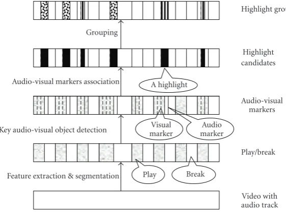
tools are used to generate a suitable representation for the content using which summaries can be created. For content that is carefully produced and edited (scripted content) such as news, movie, drama, and so forth, a representation that captures the sequence of semantic units that constitute the content has been shown to be useful. Hence, past work on summarization of scripted content has mainly focussed on coming up with a table of contents (ToC) representation as shown inFigure 1. With such a representation of the detected semantic units, a summary can be constructed using abstrac-tions (e.g., skims, keyframes) from each of the detected se-mantic units.
The following is a list of approaches towards constructing a hierarchical ToC-like representation for summarization of scripted content.
(i) News video.
(a) Detection of news story boundaries through closed caption or speech transcript analysis [1–3]. (b) Detection of news story boundaries using speaker
segmentation and face information [4,5].
(ii) Situation comedies.
(a) Detection of “physical setting” using mosaic repre-sentation of a scene [6].
(b) Detection of major cast using audio-visual cues [7].
(iii) Movie content.
(a) Detection of syntactic structures like two-speaker dialogs [8].
(b) Detection of some specific events like explosions [7].
Video
Scene
Group
Shot
Key frame
Shot boundary detection
Scene construction
Grouping
Temporal features
Spatial features Key frame extraction
Figure1: A hierarchical video representation for scripted content.
Grouping
Audio-visual markers association
Key audio-visual object detection
Feature extraction & segmentation
A highlight
Visual marker
Audio marker
Play Break
Highlight groups
Highlight candidates
Audio-visual markers
Play/break
Video with audio track Figure2: A hierarchical video representation for unscripted content.
content has mainly focussed on detecting these specific events of interest.
The following is a list of approaches from literature that detect specific events for summarization of unscripted con-tent.
(i) Sports video.
(a) Detection of domain-specific events and objects that are correlated with highlights using audio-visual cues [9–12].
(b) Unsupervised extraction of play-break segments from sports video [13].
(ii) Surveillance video.
(a) Detection of “unusual” events using object seg-mentation and tracking from video [14].
Based on the detection of such domain-specific key au-dio-visual objects (auau-dio-visual markers) that are indicative of the “highlight” or “interesting” events, we proposed a hi-erarchical representation for unscripted content as shown in
Figure 2[15]. The detected events can also be ranked
accord-ing to a chosen measure which would allow generation of summaries of desired length [16]. In this representation, for each domain the audio-visual markers are chosen manually based on intuition.
For unscripted content, the representation framework is based on the detection of specific events. Past work has shown that the play/break representation for sports can be achieved by an unsupervised analysis by bringing out repetitive temporal patterns. However, the rest of the repre-sentation units require the use of domain knowledge in the form of supervised audio-visual object detectors that are cor-related with events of interest. This necessitates a separate analysis framework for each domain in which the key audio-visual objects are chosen based on intuition. However, what is more desirable is a content-adaptive analysis and represen-tation framework that postpone content-specific processing to as late a stage as possible. Then, some challenging ques-tions towards achieving such a framework are as follows.
(i) Can we come up with a representation framework for unscripted content which requires the use of the do-main knowledge only at the last stage as the represen-tation framework for scripted content?
(ii) Discovery of what kind of patterns would support such a representation framework?
(iii) Can such a framework help in the systematic choice of the key audio-visual objects for events of interest?
In this paper, the above questions motivate us to propose a content-adaptive analysis framework aimed towards a rep-resentation framework for event discovery from unscripted multimedia. We are motivated towards an inlier/outlier-based representation for unscripted multimedia inlier/outlier-based on the observation that “interesting” events are outliers in a back-ground of usual events. In this paper, we focus on the anal-ysis of audio features for such a representation. We treat the sequence of low-level/mid-level features extracted from the input audio as a time series. Then, we discover subsequences from the input time series that are outliers. The outlier de-tection is based on eigenvector analysis of the affinity ma-trix constructed from statistical models estimated from the subsequences of the time series. The detected outliers are ranked based on the deviation from the usual. This results in a temporal segmentation of the input time series, that will henceforth be referred to as “inlier/outlier-based seg-mentation,” with observations during inliers corresponding to the usual process and observations during outliers cor-responding to the unusual events. The analysis thus far is content-adaptive (in the sense that the framework adapts to content statistics to discover the usual and unusual for a given set of parameter choices) and genre-independent, en-abling us to come up with a representation for summariza-tion without a priori knowledge. However, since the mean-ing of “interestmean-ing” is dependent on the genre, in order to present an “interesting” summary to the end user, a genre-dependent postprocessing incorporating the domain knowl-edge can be performed on the discovered outlier subse-quences.
The rest of the paper is organized as follows. In the next section, we propose our framework for event discovery using audio features in unscripted content. In Sections3,4, and5, we describe each of the components in the proposed frame-work in detail. In Section 6, we present the results of the
proposed framework on sports audio content and surveil-lance audio content. InSection 7, we present our discussion on systematic choice of key audio classes for a chosen domain before presenting our conclusions.
2. PROPOSED FRAMEWORK
With the knowledge of the domain of the unscripted con-tent, one can come up with an analysis framework with su-pervised learning tools for the generation of the hierarchical representation of events in unscripted content for summa-rization as shown inFigure 2. We propose a content adap-tive analysis framework which does not require any a priori knowledge of domain of the unscripted content. It is aimed towards an inlier/outlier-based representation of the content for event discovery and summarization as shown inFigure 3. We briefly describe the role of each component in the proposed framework as follows.
(i)Feature extraction: in this step, low-level features are extracted from the input content in order to generate a time series from which events are to be discovered. For example, the extracted features from the audio stream, could be Mel-frequency cepstral coefficients (MFCC).
(ii)Classification/clustering: in this step, the low-level fea-tures are classified using supervised models for classes that span the whole domain to generate a discrete time series of mid-level classification/clustering labels. One could also dis-cover events from this sequence of discrete labels. For exam-ple, Gaussian mixture models (GMMs) can be used to clas-sify every frame of audio into one of the following five audio classes which span most of the sounds in sports audio: ap-plause, cheering, music, speech, and speech with music. At this level, the input unscripted content is represented by a time series of mid-level classification/cluster labels.
(iii)Detection of subsequences that are outliers in a time series: in this step, we detect outlier subsequence from the time series of low-level features or mid-level classification la-bels motivated by the observation that “interesting” events are unusual events in a background of “uninteresting” hap-penings. At this level, the input content is represented by a temporal segmentation of the time series into inlier and out-lier subsequences. The detected outout-lier subsequences are il-lustrated inFigure 3asOi, 1≤i≤n.
(iv) Ranking outlier subsequences: in order to generate summaries of desired length, we rank the detected outliers with respect to a measure of statistical deviation from the in-liers. At this level, the input content is represented by a tem-poral segmentation of the time series into inlier and ranked outlier subsequences. The ranks of detected outlier subse-quences are illustrated inFigure 3asri, 1≤i≤n.
Unscripted content
Feature extraction
Outlier subsequence detection in time
series Classification/
clustering
Ranking outlier subsequences
Summarization Domain
knowledge
Summary
Representation
Video with audio track
Time series of low-level features Time series of classification/ cluster labels
Outlier subsequences Ranked outlier
subsequences
Ranked “interesting” subsequences O1 O2 O3 On−1On
r1 r2 r3 rn−1 rn
O1 O2 O3 On−1On k1 k2 km
S1 S2 Sm−1 Sm
· · ·
· · ·
Analysis
Figure3: Proposed event discovery framework for analysis and representation of unscripted content for summarization.
of commercials from the summary. At this level, the input content is represented by a temporal segmentation of the time series into inlier and ranked “interesting” outlier sub-sequences. The “interesting” outlier subsequences are illus-trated inFigure 3asSi, 1≤i≤m, with rankski. The set of “interesting” subsequences (Si)’s is a subset of outlier subse-quences (Ois).
In the following sections, we describe each of these com-ponents in detail.
3. CLASSIFICATION/CLUSTERING FRAMEWORK FOR MID-LEVEL REPRESENTATION
We extracted low-level features and model the distribution of features for classification into one of the several classes that span the whole domain of unscripted content. We took sports content as an example of unscripted content to explain the classification framework. The following sound classes span almost all of the sounds in sports domain: applause, cheering, music, speech, and speech with music. We have col-lected 679 audio clips from TV broadcasts of golf, baseball, and soccer games. This database is a subset of that in [17]. Each clip is hand-labeled into one of the five classes as ground truth: applause, cheering, music, speech, and “speech with music.” The corresponding numbers of clips are 105, 82, 185, 168, and 139. The duration of the clips differs from around 1 s to more than 10 s. The total duration is approximately 1 h and 12 min. The audio signals are all monochannel with a sampling rate of 16 kHz. We extracted 12 Mel-frequency cep-stral coefficients (MFCC) for every 8 ms frame and logarithm of energy, from all the clips in the training data. We per-formed classification experiments with varying number of MFCC coefficients and chose 12 as a tradeoffbetween com-putational complexity and performance. We trained Gaus-sian mixture models (GMMs) to model the distribution of
features for each of the sound classes. The number of mix-ture components were found using the minimum descrip-tion length principle [16]. Then, given a test clip, we ex-tract the features for every frame and assign a class label corresponding to the sound class model for which the likeli-hood of the observed features is maximum. For all the exper-iments to be described in the following sections, we use one of the following time series to discover “interesting” events at different scales:
(i) the time series of 12 MFCC features and logarithm of energy extracted for every frame of 8 milliseconds; (ii) the time series of classification labels for every frame; (iii) the time series of classification labels for every second
of audio. The most frequent frame label in one second is assigned as the label for that second.
In the following section, we describe the outlier subse-quence detection from one of the three time series defined in this section.
4. OUTLIER SUBSEQUENCE DETECTION IN TIME SERIES
Outlier subsequence detection is at the heart of the proposed framework and is motivated by the observation that “inter-esting” events in unscripted multimedia occur sparsely in a background of usual or “uninteresting” events. Some exam-ples of such events are:
(i) sports: a burst of overwhelming audience reaction in the vicinity of a highlight event in a background of commentator’s speech,
This motivates us to formulate the problem of discov-ering “interesting” events in multimedia as that of detect-ing outlier subsequences or “unusual” events by statistical modeling of a stationary background process in terms of low/mid-level audio-visual features. Note that the back-ground process may be stationary only for small period of time and can change over time. This implies that background modeling has to be performed adaptively throughout the content. It also implies that it may be sufficient to deal with one background process at a time and detect outliers. In the following subsection, we elaborate on this more formally.
4.1. Problem formulation
Letp1represent a realization of the “usual” class (P1) which
can be thought of as the background process. Letp2represent a realization of the “unusual” classP2which can be thought
of as the foreground process. Given any time sequence of observations or low-level audio-visual features from the two classes of events (P1andP2), such as
· · ·p1p1p1p1p1p2p2p1p1p1· · ·, (1) then the problem of outlier subsequence detection is that of finding the times of occurrences of realizations ofP2.
To begin with, the statistics of the classP1 are assumed
to be stationary. However, there is no assumption about the classP2. The class P2 can even be a collection of a diverse
set of random processes. The only requirement is that the number of occurrences ofP2 is relatively rare compared to
the number of occurrences of the dominant class. Note that this formulation is a special case of a more general problem, namely, clustering of a time series in which a single highly dominant process does not necessarily exist. We treat the se-quence of low/mid-level audio-visual features extracted from the video as a time series and perform a temporal segmenta-tion to detect transisegmenta-tion points and outliers from a sequence of observations.
Before we present our framework for detection of outlier subsequences, we review the related theoretical background on the graph-theoretical approach to clustering.
4.2. Segmentation using eigenvector analysis of affinity matrices
Segmentation using eigenvector analysis has been proposed in [18] for images. This approach to segmentation is related to graph-theoretic formulation of grouping. The set of points in an arbitrary feature space are represented as a weighted undirected graph where the nodes of the graph are points in the feature space and an edge is formed between every pair of nodes. The weight on each edge is the similarity between nodes. Let us denote the similarity between nodesiand jas
w(i,j).
In order to understand the partitioning criterion for the graph, let us consider partitioning it into two groupsAand
BandA∪B=V:
Ncut(A,B)= cut(A,B) asso(A,V)+
cut(A,B)
asso(B,V), (2)
where
cut(A,B)=
i∈A,j∈B
w(i,j),
asso(A,V)=
i∈A,j∈V
w(i,j). (3)
Note that cut(A,B) measures the total connection from nodes inAto all the nodes inB, whereas asso(A,V) mea-sures the total connection from nodes inAto all the nodes in the graph. It has been shown in [18] that minimizingNcut minimizes similarity between groups while maximizing as-sociation within individual groups. Shi and Malik [18] show that
min
x Ncut(x)=miny
yT(D−W)y
yTDy (4)
with the condition that yi belongs to{−1,b}. HereW is a symmetric affinity matrix of sizeN×N (consisting of the similarity between nodesiandj,w(i,j) as entries ) andDis a diagonal matrix withd(i,i)=jw(i,j).xandyare cluster indicator vectors, that is, ify(i) equals−1, then feature point “i” belongs to clusterA, else clusterB. It has also been shown that the solution to the above equation is same as the solution to the following generalized eigenvalue system ifyis relaxed to take on real value:
(D−W)y=λDy. (5) This generalized eigenvalue system is solved by first trans-forming it into the standard eigenvalue system by substitut-ingz=D1/2yto get
D−1/2(D−W)D−1/2z=λz. (6)
It can be verified thatz0 = D1/2−→1 is a trivial solution with eigenvalue equal to 0. The second generalized eigenvec-tor (the smallest nontrivial solution) of this eigenvalue sys-tem provides the segmentation that optimizesNcutfor two clusters. In this paper, we use the term “the cluster indicator vector” interchangeably with “the second generalized eigen-vector of the affinity matrix.”
Also, note that although this method of segmentation us-ing eigenvector analysis has been introduced by Shi and Ma-lik, in the context of image segmentation, it also can be used to segment a time series of audio features as we will see later. The key is to compute an affinity from the input times series of audio features in a meaningful way. Thereafter, the nature of the source from which the affinity matrix is computed has no influence on the mathematics.
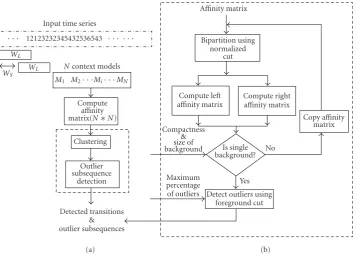
4.3. Proposed outlier subsequence detection in time series
Given the problem of detecting times of occurrences of P1
andP2from a time series of observations fromP1andP2, we
propose the following time series clustering framework.
Input time series
· · · 12123232345432536543 · · · ·
WL WL WS
Ncontext models M1 M2· · ·Mi· · ·MN
Compute affinity matrix(N∗N)
Clustering Outlier subsequence
detection
Affinity matrix
Detected transitions & outlier subsequences
(a)
Bipartition using normalized
cut
Compute left affinity matrix
Compute right affinity matrix
Copy affinity matrix Is single
background? Compactness
& size of
background No
Yes Maximum
percentage
of outliers Detect outliers using foreground cut
(b) Figure4: Proposed outlier subsequence detection framework.
sequence of observations) be referred to as a context
Ci.
(2) Compute a statistical model Mifrom the time series observations within eachCi.
(3) Compute the affinity matrix for the whole time series using the context models and a commutative distance metric (d(i,j)) defined between two context models (MiandMj). Each element,A(i,j), in the affinity ma-trix ise−d(i,j)/2σ2, whereσ is a parameter that controls how quickly affinity falls offas distance increases. (4) The computed affinity matrix represents an undirected
graph where each node is a context model and each edge is weighted by the similarity between the nodes connected by it. Then, we can use a normalized cut solution to identify distinct clusters of context mod-els and “outliers context modmod-els” that do not belong to any of the clusters. Note that the second general-ized eigenvector of the computed affinity matrix is an approximation to the cluster indicator vector, as dis-cussed inSection 4.2.
Figure 4illustrates the proposed framework. The portion
ofFigure 4(b) is a detailed illustration of the two blocks: clus-tering and outlier detection in Figure 4(a). In this frame-work, there are two key issues, namely, the statistical model for the context and the choice of the two parameters, the context window size (WL) and the sliding window size (WS)
(seeFigure 4(a)). The choice of the statistical model for the
time series sample in a context would depend on the underly-ing background process. A simple unconditional probability density function(PDF) estimate would suffice for a memo-ryless background process. However, if the process has some
memory, the chosen model would have to account for it. For instance, a hidden Markov model (HMM) would provide a first-order approximation.
The choice of the two parameters (WLandWS) would be determined by the confidence with which a subsequence is declared to be an outlier.The size of the windowWL deter-mines the reliability of the statistical model of a context.The size of the sliding factor, WS, determines the resolution at which the outlier is detected.
Before we discuss the choice of these parameters, we show some results on synthetic time series data.
4.4. Results with synthetic time series data
In this section, first, we show the effectiveness of the pro-posed outlier subsequence detection framework using syn-thetic time series data. Second, we compare the normalized cut with other clustering approaches for outlier subsequence detection from time series.
The synthetic time series generation framework is shown inFigure 5.
In this framework, we have a generative model for both P1andP2and the dominance of one over the other can also
be governed by a probability parameter. It is also possible to control the percentage of observations fromP2in a given
context.
There are four possible scenarios one can consider with the proposed generative model for label sequences.
Case 1. Sequence completely generated fromP1. This case is
Case 2. Sequence dominated by observations from P1, that
is,P(P1)P(P2). An example for this case is a time series
of audio class labels for each second of a news program. Here a burst of music and speech-with-music audio class labels corresponds to commercial messages (P2) in the recording.
The speech background in the news program corresponds to the usual background process,P1.
Case 3. Sequence dominated by observations from P1, that
is,P(P1) P(P2) ≈P(P3) ≈ P(P4), whereP2,P3,P4are
foreground processes. An example for this case is a time series of audio class labels for each second from a sports broadcast. In this case, a burst of audience-reaction audio class labels may correspond toP2and a burst of music audio class labels
may correspond toP3.
Case 4. Sequence with observations from P1 and P2 with
no single dominant class with a number of foreground pro-cesses, that is,P(P1)≈P(P2) and (P(P1)+P(P2))(P(P3)+ P(P4)). An example for this case is a time series of features
from a clip that has two different genres, say news and sports.
4.4.1. Performance of the normalized cut forCase 2
In this section, we show the effectiveness of normalized cut forCase 2, that is, whenP(P1)P(P2). Without loss of
gen-erality, let us consider an input discrete time series with an al-phabet of three symbols (1, 2, 3) generated from two HMMs (P1andP2).
The parameters ofP1(the state transition matrix (A), the
state observation symbol probability matrix (B), the initial state probability matrix (Π)) are:
AP1= ⎛ ⎜ ⎝
0.3069 0.0353 0.6579 0.0266 0.9449 0.0285 0.5806 0.0620 0.3573
⎞ ⎟ ⎠,
BP1= ⎛ ⎜ ⎝
0.6563 0.2127 0.1310 0.0614 0.0670 0.8716 0.6291 0.2407 0.1302
⎞ ⎟ ⎠,
ΠP1=
0.1 0.8 0.1.
(7)
The parameters ofP2are
AP2=
0.9533 0.0467 0.2030 0.7970
,
BP2=
0.0300 0.8600 0.1100 0.3200 0.5500 0.1300
,
ΠP2=
0.8 0.2.
(8)
Then, using the generative model shown inFigure 5with
P(P1) = 0.8 and P(P2) = 0.2 we generate a discrete time
series of symbols as shown inFigure 6(a).
We sample this series uniformly using a window size of
WL =200 and a step size ofWS =50. We use the observa-tions within every context to estimate an HMM with 2 states. Using the distance metric defined below for comparing two HMMs, we compute the distance matrix for the whole time
series. Given two context models (λ1andλ2) with observa-tion sequencesO1andO2, respectively, we define
Dλ1,λ2
= 1
WL
logPO1|λ1
+ logPO2|λ2
−logPO1|λ2
−logPO2|λ1
.
(9)
The computed distance matrix,D, is normalized to have values between 0 and 1. Then, using a value ofσ =0.2, we compute the affinity matrix,A, whereA(i,j) = e−d(i,j)/2σ2. The affinity matrix is shown inFigure 6(b). We compute the second generalized eigenvector of this affinity matrix as a solution to cluster indicator vector. Since the cluster indi-cator vector does not assume two distinct values, a thresh-old is applied on the eigenvector values to get the two clus-ters. In order to compute the optimal threshold, normalized cut value is computed for the partition resulting from each candidate threshold between the range of eigenvector values. The optimal threshold is selected as the threshold at which normalized cut value is minimum as shown inFigure 6(c). The corresponding second generalized vector and its opti-mal partition is shown inFigure 6(d). The detected outliers are at times of occurrences ofP2.Figure 6(e)marks the
de-tected outlier subsequences in the original time series based on normalized cut. It can be observed that the outlier sub-sequences have been detected successfully without having to set any threshold manually. Also, note that since all outlier subsequences are from the same foreground process (P2), the
normalized cut solution found the outlier subsequences. In general, as we will see later, when the outliers are from more than one foreground process (Case 3), the normalized cut so-lution may not perform as well. This is because each outlier can be different in its own way and it is not right to emphasize association between the outlier cluster members as normal-ized cut does.
In the following subsection, we show the performance of other competing clustering approaches for the same task of detecting outlier subsequences using the computed affinity matrix.
4.4.2. Comparison with other clustering approaches forCase 2
After constructing the affinity matrix in step (3), step (4) finds clusters in model space. Instead of using normalized cut solution for clustering, one could use one of the follow-ing three methods for clusterfollow-ing.
Clustering using alphabet-constrainedK-means
Choose sequence generated from
P1orP2. IfP2, fill sequence frommtoL
with labels fromP1
Generate a label sequence of lengthm
(uniform∼(0, L)) withP2 Generate a label
sequence of lengthL withP1
Sequence of lengthL L
P1
or
Pz P1
P1
m L−m P(p2)
P2 P(p1)
1
Figure5: Generative model for synthetic time series with one background process and one foreground process.
Given that there is one dominant cluster and the distance matrix, we can use the following algorithm to detect outliers.
(1) Find the row in the distance matrix for which the aver-age distance is minimum. This is the centroid model. (2) Find the semi-Hausdorff distance between the
cen-troid model and the cluster members. The semi-Hausdorffdistance, in this case, is simply the maxi-mum of all the distances computed between the cen-troid model and the cluster members. Hence, semi-Hausdorffdistance would be much larger than the av-erage distance if there are any outliers in the cluster members.
(3) Remove the farthest model and repeat step (2) until the difference between average distance and Hausdorff distance is less than a chosen threshold.
(4) The remaining cluster members constitute the inlier models.
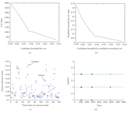
For more than one cluster, repeat steps (1)–(3) on the complementary set which does not include members of the detected cluster. For more details on alphabet-constrainedk -means, please see [19].Figure 7(a)shows the distance matrix values of the row that is corresponding to the centroid row. By using a threshold on the difference between average dis-tance and Hausdorffdistance, we detect outlier subsequences as shown inFigure 7(b).
Clustering based on dendrogram
Given the pairwise distance matrix one can perform a bottom-up agglomerative clustering. At the start, each point is considered to be an individual cluster. By merging two closest clusters at every level until there is only one cluster, a dendrogram can be constructed as shown inFigure 8(a). Then, by partitioning this dendrogram at a particular height, one can get the individual clusters. The criteria for evaluating
a partition could be similar to what normalized cut tries to optimize. There are several choices for creating partitions in the dendrogram and one has to exhaustively compute the objective function value for each partition and choose the one that is optimal. For more details on dendrogram-based agglomerative clustering, please see [20]. For example, by manually selecting a threshold of 5.5 for the height, we can detect outlier subsequences as shown inFigure 8(b). As can be seen from the figure, there are some false alarms and misses in the detected outlier subsequences as the threshold was chosen manually.
Clustering based on factorization of the affinity matrix
As mentioned earlier, minimizingNcut minimizes similarity between groups while maximizing association within the in-dividual groups. Perona and Freeman modified the objec-tive function of the normalized cut to discover a “salient” foreground object from an unstructured background. Since the background is assumed to be unstructured, the objective function of normalized cut was modified as follows:
Ncut∗(A,B)=
cut(A,B)
asso(A,V), (10)
where clusterAis the foreground and clusterBis the back-ground. Note that the objective function only emphasizes the compactness of foreground cluster while minimizing simi-larity between clusterAand clusterB. Perona and Freeman solved this optimization problem by setting up the problem in the same way as in the normalized cut. The steps of the resulting “foreground cut” algorithm is as follows [21].
0 1000 2000 3000 4000 5000 6000 7000 8000 1
1.5 2 2.5 3 3.5 4
Observations fromP1
Observations fromP2
Time
Sy
m
b
o
l
(a)
20 40 60 80 100 120 140 160 160
140 120 100 80 60 40 20
(b)
Candidate normalized cut threshold
N
o
rmaliz
ed
cu
t
o
bjecti
ve
functio
n
−0.005 0 0.005 0.01 0.015 0.02 0.025 0.03 0.035 0.65
0.7 0.75 0.8 0.85 0.9 0.95 1
(c)
0 20 40 60 80 100 120 140 160
−0.01
−0.005 0 0.005 0.01 0.015 0.02 0.025 0.03 0.035
Outliers
Inliers
Time index of context model
Cl
ust
er
indicat
or
vo
lu
me
(d)
0 1000 2000 3000 4000 5000 6000 7000 8000 1
1.5 2 2.5 3 3.5 4
Time
Sy
m
b
o
l
(e)
Figure6: Performance of normalized cut on synthetic time series forCase 2. (a) Input time series of discrete labels. (b) The affinity matrix A. (c) Normalized cut value. (d) Second generalized eigenvector. (e) Outlier subsequence detection using normalized cut.
(ii) Compute the vectoru=SU1where1is a column vec-tor of ones.
0 20 40 60 80 100 120 140 160 0
50 100 150 200 250
Time index of context model
Cl
ust
er
indicat
or
val
u
e
Outliers
(a)
0 1000 2000 3000 4000 5000 6000 7000 8000 1
1.2 1.4 1.6 1.8 2 2.2 2.4 2.6 2.8 3
Sy
m
b
o
l
Time (b) Figure7: Performance ofK-means on synthetic time series forCase 2.
9 8 7 6 5 4 3 2 1 0
Data index
Distanc
e
(a)
0 1000 2000 3000 4000 5000 6000 7000 8000 1
1.5 2 2.5 3 3.5 4
Sy
m
b
o
l
Time (b)
Figure8: Performance of dendrogram cut on synthetic time series forCase 2. (a) Dendrogram. (b) Outlier subsequence detection using the dendrogram.
(v) Threshold x, to obtain the foreground and back-ground.xis similar to the cluster indicator vector in normalized cut.
The threshold in the last step can be obtained in the same way as it was obtained for normalized cut.
For the problem at our hand, the situation is reversed, that is, the background is structured while the foreground can be unstructured. Therefore, the same “foreground cut” solution should apply as the modified objective function is
Ncut∗∗(A,B)=
cut(A,B)
asso(B,V). (11) However, a careful examination of the modified objec-tive function would reveal that the term in the denominator asso(B,V) would not be affected drastically by changing
Cu
t
va
lu
e
Candidate threshold for cut
−00.09−0.08 −0.07 −0.06 −0.05 −0.04 −0.03 −0.02 500
1000 1500 2000 2500 3000 3500 4000
(a)
Candidate threshold for modified normalized cut
M
o
dified
nor
m
aliz
ed
cut
val
ue
−00.09−0.08 −0.07 −0.06 −0.05 −0.04 −0.03 −0.02 0.05
0.1 0.15 0.2 0.25 0.3 0.35 0.4 0.45
(b)
0 20 40 60 80 100 120 140 160
−0.1
−0.09
−0.08
−0.07
−0.06
−0.05
−0.04
−0.03
−0.02
−0.01 Outliers
Inliers
Cl
ust
er
indicat
or
val
u
e
Time index of context model (c)
Time
Sy
m
b
o
l
0 1000 2000 3000 4000 5000 6000 7000 8000 1
1.5 2 2.5 3 3.5 4
(d)
Figure9: Performance of modified normalized cut on synthetic time series forCase 2. (a) The value of the objective function cut for
candidate threshold values. (b) Modified normalized cut (affinity matrix factorization). (c), (d) Outlier subsequence detection based on
affinity matrix factorization.
is met. For example, the stopping criterion could either be based on percentage of foreground points or based on the radius of the background cluster.
As shown in this section, all of the competing clustering approaches need a threshold to be set for detecting outlier subsequences. The alphabet-constrainedk-means algorithm needs the knowledge of the number of the clusters and a threshold on the difference between the average distance and the semi-Hausdorff distance. The dendrogram-based agglomerative clustering algorithm needs a suitable objec-tive function to evaluate and select the partitions. The fore-ground cut (modified normalized cut) algorithm finds small isolated clusters and can be recursively repeated on the back-ground until the radius of the backback-ground cluster is smaller than a chosen threshold. Therefore, for the case of a single dominant process with outlier subsequences from a single foreground process, the normalized cut outperforms other clustering approaches.
In the following section, we consider the next case where there can be multiple foreground processes generating obser-vations against a single dominant background process.
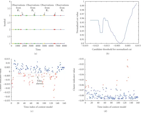
4.4.3. Performance of normalized cut forCase 3
The input time series forCase 3 is generated using a single dominant background processP1 and three different
fore-ground processes (P2,P3,P4) andP(P1)P(P2) +P(P3) + P(P4).P(P1) was set to be 0.8 as inCase 2.Figure 10(a)shows
the input time series. As mentioned earlier, since normalized cut emphasizes the association between the cluster mem-bers for the two clusters resulting from the partition, there are false alarms from the processP1 in the cluster
contain-ing outliers.Figure 10(b)shows the normalized cut value for candidate threshold values. There are two minima in the ob-jective function but the global minimum corresponds to the threshold that results in an outlier cluster with false alarms.
0 1000 2000 3000 4000 5000 6000 7000 8000 Time
1 1.5 2 2.5 3 3.5 4
Sy
m
b
o
l
Observations from
P1
Observations from
P2
Observations from
P3
Observations from
P4
(a)
−0.035 −0.025 −0.015 −0.005 0.005 0.015 Candidate threshold for normalized cut 0.9
0.91 0.92 0.93 0.94 0.95 0.96 0.97 0.98 0.99 1
N
o
rm
aliz
ed
cut
value
(b)
0 20 40 60 80 100 120 140 160 Time index of context model
−0.035
−0.03
−0.025
−0.02
−0.015
−0.01
−0.005 0 0.005 0.01 0.015
False alarms
Cl
ust
er
indicat
or
val
u
e
(c)
0 20 40 60 80 100 120 140 160
−0.09
−0.08
−0.07
−0.06
−0.05
−0.04
−0.03
−0.02
−0.01
Cl
ust
er
indicat
or
val
u
e
Time index of context model (d)
Figure10: Performance comparison of normalized cut and modified normalized cut on synthetic time series forCase 3. (a) The input time series. (b) The normalized cut value for candidate threshold values. (c) The partition corresponding to the global minimum threshold. (d) Modified normalized cut (foreground cut) applied to the same input series.
minimum threshold. On the other hand, when modified nor-malized cut (foreground cut) is applied to the same input time series, it detects the outliers without any false alarms as shown inFigure 10(d)as the objective function does not em-phasize association between the foreground processes.
4.4.4. Hierarchical clustering using normalized cut forCase 4
From the experiments on synthetic time series for Cases2
and3, we can make the following observations.
(i) The normalized cut solution is good for detecting dis-tinct time series clusters (backgrounds) as the thresh-old for partitioning is selected automatically.
(ii) The foreground cut solution is good for detecting out-lier subsequences from different foreground processes that occur against a single background.
Both of these observations lead us to a hybrid solu-tion which uses both normalized cut and foreground cut
for handling the more general situation inCase 4. InCase 4, there is no single dominant background process and the out-lier subsequences are from different foreground processes.
Figure 11(a)shows the input time series forCase 4. There are
two background processes and three foreground processes. Given this input time series and the specifications of a single background in terms of its “compactness” and “size relative to the whole time series” and the maximum percent-age of outlier subsequences, we use the following algorithm to detect outlier subsequences.
(1) Use normalized cut recursively to first identify all indi-vidual background processes. The decision of whether or not to split a partition further can be automatically determined by computing the stability of normalized cut as suggested in [18] or according to the “compact-ness” and “size” constraint.
0 1000 2000 3000 4000 5000 6000 7000 8000 1
1.5 2 2.5 3 3.5 4
Time
Sy
m
b
o
l
Observations fromP1
Observations fromP3
Observations fromP2
Observations fromP4
(a)
Cl
ust
er
indicat
or
Clust
er
lab
el
Time
Time index of context model
0 20 40 60 80 100 120 140 160
−0.02
−0.01 0 0.01 0.02 0.03
0 20 40 60 80 100 120 140 160 1
1.2 1.4 1.6 1.8 2
(b)
Cl
ust
er
indicat
or
Clust
er
lab
el
Time
Time index of context model
0 10 20 30 40 50 60 70 80 90
−0.02 0 0.02 0.04 0.06 0.08 0.1 0.12
0 20 40 60 80 100 120 140 160 1
1.5 2 2.5 3 3.5 4
(c)
Clust
er
lab
el
Time
0 20 40 60 80 100 120 140 160
−1
−0.5 0 0.5 1 1.5 2 2.5 3
(d)
Figure11: Performance of hybrid (normalized cut and foreground cut) approach on synthetic time series forCase 4. (a) The input time
series. (b) Top: result of normalized cut (root partition, 1 minute, Ncut=8.275415e - 001); bottom: corresponding temporal
segmenta-tion (left radius=0.240746, right radius=1.414331). (c) Top: result of normalized cut (p1-1 partition, 2 minutes, Ncut=8.439419e - 001);
bottom: corresponding temporal segmentation (left radius=0.663607, right radius=0.594490). (d) Final detected outlier subsequences using
foreground cut on individual background clusters.
The “compactness” of a cluster can be specified by com-puting its radius using the pairwise affinity matrix as given below:
r= max
1≤i≤N
A(i,i)−
2
N
N
j=1
A(i,j)
+
1
N2 N
k=1 N
j=1
A(k,j)
.
(12)
HereNrepresents the number of cluster members. The first term represents the self affinity and is equal to 1. The second term represents the average affinity of theith cluster mem-ber with others and the last term is average affinity between all the members of the cluster. The computed value of r is guaranteed to be between 0 and 1.
For this input time series, we specified the following pa-rameters: compactness of the background in terms of its ra-dius≤0.5, relative size of background with respect to the size of whole time series≥0.35, and maximum outlier percent-age was set to 20%. Figure11(b)and11(c)show the result
of normalized cut and the corresponding temporal segmen-tation of the input time series.Figure 11(d)shows the final detected outlier subsequences using foreground cut on indi-vidual background clusters.
Now that we have shown the effectiveness of outlier sub-sequence detection on synthetic time series, we will show its performance on the time series obtained from audio data of sports and surveillance content in the experimental results section. In the following section, we analyze how the size of window used for estimating a context model (WL) deter-mines the confidence on the detected outlier. The confidence measure is then used to rank the detected outliers.
5. RANKING OUTLIERS FOR SUMMARIZATION
Recall that in the proposed outlier subsequence detec-tion framework, we sample the input time series on a uni-form grid of size WL and estimate the parameters of the background process from the observations withinWL. Then, we measure how different it is from other context mod-els. The difference is caused either by the observations from P2 within WL or by the variance of the estimate of the background model. If the observed difference between two context models is “significantly higher than allowed” by the variance of the estimate itself, then we are “somewhat confi-dent” that it was due to the corruption of one of the contexts with observations fromP2.
In the following, before we quantify what is “significantly higher than allowed” and what is “somewhat confident” in termsWLfor two types of background models that we will be dealing with, we will review kernel density estimation.
5.1. Kernel density estimation
Given a random samplex1,x2,. . .,xnofnobservations ofd -dimensional vectors from some unknown density (f) and a kernel (K), an estimate for the true density can be obtained
f(x)= 1
nhd n
i=1
K
x−xi
h
, (13)
where h is the bandwidth parameter. If we use the mean squared error (MSE) as a measure of efficiency of the den-sity estimate, the tradeoffbetween bias and variance of the estimate can be seen as shown below:
MSE=E f(x)−f(x)2=Var f(x)+Bias f(x)2.
(14) It has been shown in [22] that the bias is proportional toh2and the variance is proportional ton−1h−d. Thus, for a fixed bandwidth estimator one needs to choose a value of
hthat achieves the optimal tradeoff. We use a data-driven bandwidth selection algorithm proposed in [23] for the es-timation. The proposed scheme uses the plug-in rule and has been shown to be superior to other approaches for fixed bandwidth estimation. For details on the plug-in rule, please see the appendix of [24].
5.2. Confidence measure for outliers with binomial and multinomial PDF models for the contexts
For the background process to be modeled by a binomial or multinomial PDF, the observations have to be discrete. With-out loss of generality, let us represent the set of 5 discrete labels (the alphabet of P1 andP2) by S = {A,B,C,D,E}.
Given a context consisting of WLobservations from S, we can estimate the probability of each of the symbols inSusing the relative frequency definition of probability.
Let us represent the unbiased estimator for probability of the symbolAaspA.pAis a binomial random variable but can be approximated by a Gaussian random variable with mean aspAand variance as
pA(1−pA)/WLwhenWL≥30. As mentioned earlier, in the proposed framework we are interested in knowing the confidence interval of the random
variable,d, which measures the difference between two es-timates of context models. For mathematical tractability, let us consider the Euclidean distance metric between two PDFs, even though it is only a monotonic approximation to a rig-orous measure such as the Kullback-Leibler distance:
d=
i∈S
pi,1−pi,2
2
. (15)
Here pi,1andpi,2represent the estimates for the probability ofith symbol from two different contexts of sizeWL. Since
pi,1and pi,2 are both Gaussian random variables,dis aχ2 random variable with ndegrees of the freedom wherenis the cardinality of the setS.
Now, we can assert with certain probability,
Pc=
U
L fχ 2
n(x)dx, (16)
that any estimate ofd(d) lies in the interval [L,U]. In other words, we can be Pc confident that the difference between two context model estimates outside this interval was caused by the occurrence ofP2in one of the contexts. Also, we can
rank all the outliers using the probability density function of
d.
To verify the above analysis, we generated two contexts of size WL from a known binomial or multinomial PDF (assumed to be the background process). Let us represent the models estimated from these two contexts byM1andM2, respectively. Then, we use Bootstrapping and kernel density estimation to verify the analysis on PDF ofdas shown below.
(1) GenerateWLsymbols fromM1andM2.
(2) Reestimate the model parameters (pi,1andpi,2) based on the generated data and compute the chosen dis-tance metric (d) for comparing two context models. (3) Repeat steps (1) and (2)Ntimes.
(4) Use kernel density estimation to get the PDF ofd,pi,1, andpi,2.
Figure 12(a) shows the estimated PDFs for binomial
model parameters for two contexts of the same size (WL). It can be observed thatpi,1andpi,2are Gaussian random vari-ables in accordance with Demoivre-Laplace theorem [25].
Figure 12(b)shows estimated PDFs of the defined distance
metric for different context sizes. One can make the follow-ing two observations:
(i) the PDF of the distance metric isχ2with two degrees of freedom in accordance with our analysis;
(ii) the variance of the distance metric decreases as the number of observations within the context increases from 100 to 600.
Figure 12(c) shows the PDF estimates for the case of
multinomial PDF as a context model with different context sizes (WL). Here, the PDF estimate for the distance metric isχ2with 4 degrees of freedom which is consistent with the number of symbols in the used multinomial PDF model.
−00.1−0.05 0 0.05 0.1 0.15 0.2 0.25 0.3 0.35 0.4 0.5
1 1.5 2 2.5 3
×10−3
p1estimate from context 1
p1estimate from context 2 Difference between
estimates
(a)
Chi square with degree 2
1 2 3 4 5 6 7 8 9 10 11
×10−2 0
0.5 1 1.5 2 2.5 3 3.5 4
×10−3
100 200 400 600
(b)
Chi square with degree 4
0 0.02 0.04 0.06 0.08 0.1 0.12 0.14 0
0.5 1 1.5 2 2.5 3 3.5
4 ×10
−3
100 200 400 600
(c)
0 0.5 1 1.5 2 2.5 3 3.5 4 4.5 0
0.5 1 1.5 2 2.5 3 3.5×10
−3
100 200
400 600
(d)
−00.5 0 0.5 1 1.5 2 2.5 3
1 2 3 4 5 6 7×10
−3
100 200
600 400
(e)
Figure12: PDFs of distance metrics for different background models. (a) PDF of an estimate of a context model parameter (context size of
400 symbols), (b) PDF of distances for a binomial context model for different context sizes, (c) PDF of distances for a multinomial context
model for different context sizes, (d) PDF of distances for a GMM as a context model, and (e) PDF of distances for an HMM as a context
model.X-axis for value of the random variable,Y-axis for probability density.
for a chosenWL, one can compute the PDF of the distance metric, and any outlier caused by the occurrence of symbols from another process (P2) would result in a sample from the
tail of this PDF. This would let us quantify the “unusualness” of an outlier in terms of its cumulative distribution function (CDF) value.
In the next subsection, we perform a similar analysis for HMMs and GMMs as context models.
5.3. Confidence measure for outliers with GMM and HMM models for the contexts
When the observations of the memoryless background pro-cess are not discrete, one would model its PDF using a
(λ1andλ2with observation sequencesO1andO2, resp.):
Dλ1,λ2
= 1
WL
logPO1|λ1
+ logPO2|λ2
−logPO1|λ2
−logPO2|λ1
.
(17)
The first two terms in the distance metric measure the likelihood of training data given the estimated models. The last two cross-terms measure the likelihood of observingO2 underλ1and vice versa. If the two models are different, one would expect the cross-terms to be much smaller than the first two terms. Unlike inSection 5.2, the PDF ofD(λ1,λ2) does not have a convenient parametric form. Therefore, we directly apply bootstrapping to get several observations of the distance metric and use kernel density estimation to get the PDF of the defined distance metric.
Figure 12(d)shows the PDF of the log likelihood diff
er-ences for GMMs for different sizes of context. Note that the support of the PDF decreases asWLincreases from 100 to 600. The reliability of the two context models for the same background process increases as the amount of training data increases and hence the variance of normalized log likelihood difference decreases. Therefore, again it is possible to quan-tify the “unusualness” of outliers caused by corruption of ob-servations from another process (P2). Similar analysis shows
that the same observations hold for HMMs as context mod-els as well.Figure 12(e)shows the PDF of the log likelihood differences for HMMs for different sizes of the context.
5.4. Using confidence measures to rank outliers
In the previous two sections, we looked at the estimation of the PDF of a specific distance metric for context mod-els (memoryless modmod-els and HMMs) used in the proposed framework. Then, for a given time series of observations from the two processes (P1andP2), we compute the affi
n-ity matrix for a chosen size ofWLfor the context model. We use the second generalized eigenvector to detect inliers and outliers. Then, the confidence metric for an outlier context
Mjis computed as
pMj∈O
= 1
#I
i∈I
Pd,i
d≤dMi,Mj
, (18)
wherePd,iis the density estimate for the distance metric us-ing the observations in the inlier contexti.OandIrepresent the set of outliers and inliers, respectively, and # refers to car-dinality operator.
6. EXPERIMENTAL RESULTS
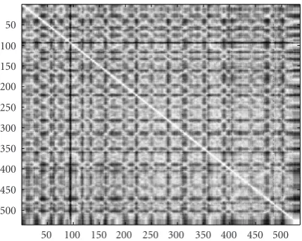
In this section, we present the results of the proposed frame-work with two different content genres mainly using low-level audio features and semantic audio classification labels at the “8 ms frame level” and “one-second level.” The pro-posed framework has been tested with a total of 12 hours of soccer, baseball, and golf content from Japanese, Amer-ican, and Spanish broadcasts. For surveillance, we chose 1.5
50 100 150 200 250 300 350 400 450 500 500
450 400 350 300 250 200 150 100 50
Figure13: Affinity matrix for a 3-hour-long British open golf game using one-second classification labels.
hours of elevator surveillance data and 2.5 hours of traffic in-tersection video. To our knowledge, this is the first time that outlier-detection-based methods have been applied for audio event discovery in sports and surveillance.
6.1. Results with sports audio content
As mentioned earlier, there are three possible choices for time series analysis from which events can be discovered using the proposed outlier subsequence detection framework. They are
(i) low-level MFCC features;
(ii) frame-level audio classification labels; (iii) one-second-level audio classification labels.
In the following subsections, we show the pros and cons of using each of these time series for event discovery with some example clips from sports audio. Since the one-second-level classification label time series is a coarse representation, we can detect commercials as outliers and extract the pro-gram segments from the whole video using the proposed framework. For discovering highlight events (for which the time span is only in the order of few seconds), we use a finer scale time series representation such as the low-level features and frame-level labels.
6.1.1. Outlier subsequence detection using
one-second-backgroundlevel labels to extract program segments
dark regions against a single background. The dark regions, with low affinity values with the rest of the regions (outliers), were verified to be times of occurrences of commercial sec-tions. Since we use the time series of the labels at one-second resolution, the detected outliers give a coarse segmentation of the whole video into two clusters: the segments that repre-sent the program and the segments that reprerepre-sent the com-mercials. Also, such a coarse segmentation is possible only because we used a time series of classification labels instead of low-level features. Furthermore, the use of low-level audio features at this stage may bring out some fine-scale changes that are not relevant for distinguishing program segments from nonprogram segments. For instance, low-level features may distinguish two different speakers in the content while a more general speech label would group them as one.
6.1.2. Outlier subsequence detection from the extracted program segments
Highlight events together with audience reaction in sports video last for only a few seconds. This implies that we can-not look for “interesting” events using the one-second-level classification labels to extract highlight events. If we use one-second-level classification labels, the size of WL has to be small enough to detect events at that resolution. However, our analysis on the confidence measures earlier indicates that a small value of WL would lead to a less reliable context model thereby producing a lot of false alarms. Therefore, we are left with the following two options:
(1) to detect outlier subsequences from the time series of frame-level classification labels instead of second-level labels;
(2) to detect outlier subsequences from the time series of low-level MFCC features.
Clearly, using the frame-level classification labels is com-putationally more efficient. Also, as pointed out earlier, working with labels can suppress irrelevant changes (e.g., speaker changes) in the background process. Figure 14(a)
shows the cluster indicator vector for a section of golf pro-gram segment. The size ofWLused was equal to 8 seconds of frame level classification labels with a step size of 4 sec-onds. The context model used for classification labels was a 2-state HMM. In the case of low-level features, the size of
WLwas equal to 8 seconds of low-level features with a step size of 4 seconds (seeFigure 14(b)). The context model was a 2-component GMM. Note that there are outliers at times of occurrences of applause segments in both cases. In the case of outlier detection from low-level features, there were at least two clusters of speech as indicated by the plot of eigenvector and affinity matrix. Speech 3 (marked in the fig-ure) is an interview section where a particular player is be-ing interviewed. Speech 1 is the commentator’s speech it-self during the game. Since we used low-level features, these time segments appear as different clusters. However, the clus-ter indicator vector from frame-level labels time series affi n-ity matrix shows a single speech background from the 49th
minute to the 54th minute. However, the outliers from the 47th minute to the 49th minute in the frame-level time se-ries were caused by misclassification of speech in “windy” background as applause. Note that the low-level feature time series does not have this false alarm. In summary, low-level feature analysis is good only when there is a stationary back-ground process in terms of low-level features. In this exam-ple, stationarity is lost due to speaker changes. Using a frame-level label time series, on the other hand, is susceptible to noisy classification and can bring out false outliers.
Figure14(c) and14(d) show the outliers in the frame labels time series and the low-level features time series re-spectively, for 10 minutes of a soccer game with the same set of parameters as for the golf game. Note that both of them show the goal scoring moment as an outlier. However, the background model of the low-level features time series has a smaller variance than the background model of the frame la-bels time series. This is mainly due to the classification errors at the frame levels for soccer audio.
In the next subsection, we present our result on inlier/ outlier-based representation for a variety of sports audio content.
6.2. Inlier/outlier-based representation and ranking of the detected outliers
In this section, we show the results of the outlier detection and ranking of the detected outliers. For all the experiments in this section, we have detected outliers from the low-level features time series to perform an inlier/outlier-based seg-mentation of every clip. The parameters of the proposed framework were set to the following: context window size (WL) = 8 seconds, step size (WS) = 4 seconds, frame rate at which MFCC features are extracted=125 frames per sec-ond, maximum percentage of outliers=20%, compactness constraint on the background=0.5, relative time span con-straint on the background = 0.35, and the context model is a 2-component GMM. They were not changed for each genre or clip of video. The first three parameters (WL,WS,
frame rate) pertain to the affinity matrix computation from the time series for a chosen context model. The fourth pa-rameter (maximum percentage of outliers) is an input to the system for the inlier/outlier-based representation. The sys-tem then returns a segmentation with at most the specified maximum percentage of outliers. The fifth and sixth param-eters (compactness and relative size) help in defining what a background is.
47 48 49 50 51 52 53 54 55
−0.02
−0.01 0 0.01 0.02 0.03 0.04 0.05 0.06
Applause
Speech Speech in rainy
background misclassified as applause
Cl
ust
er
indicat
or
val
u
e
Time (min) (a)
47 48 49 50 51 52 53 54 55
−0.04
−0.03
−0.02
−0.01 0 0.01 0.02 0.03
Speech 1 Speech 2
Speech 3
Applause
Cl
ust
er
indicat
or
val
u
e
Time (min) (b)
80 81 82 83 84 85 86 87 88 89 90
−0.06
−0.05
−0.04
−0.03
−0.02
−0.01 0 0.01 0.02
Cheering
Goal scoring & cheering Cheering Speech in noisy background
Cl
ust
er
indicat
or
val
u
e
Time (min) (c)
80 81 82 83 84 85 86 87 88 89 90
−0.14
−0.12
−0.1
−0.08
−0.06
−0.04
−0.02 0 0.02
Cheering
Goal scoring & cheering Speech in noisy background
Cl
ust
er
indicat
or
val
u
e
Time (min) (d)
0 5 10 15 20 25 30
−0.12
−0.1
−0.08
−0.06
−0.04
−0.02 0 0.02 0.04
Background
Robbery & screaming
Cl
ust
er
indicat
or
val
u
e
Time (min) (e)
2 4 6 8 10 12 14
−6
−5
−4
−3
−2
−1 0 1 2 3 4
×10−3
Ambulance sirens, cop car’s sirens, etc.
Background with cars passing intersection normally
Cl
ust
er
indicat
or
val
u
e
Time (min) (f)
Figure14: Comparison of outlier subsequence detection with low-level audio features and frame-level classification labels for sport and surveillance: (a) outlier subsequences in frame labels time series for golf; (b) outlier subsequences in low-level features time series for golf; (c) outlier subsequences in frame labels time series for soccer; (d) outlier subsequences in low-level features time series for soccer; (e) outlier
subsequences in low-level features time series for elevator surveillance; (f) outlier subsequences in low-level Features time series for traffic