Convex Relaxation for Low-Dimensional Representation:
Phase Transitions and Limitations
Thesis by Samet Oymak
In Partial Fulfillment of the Requirements for the Degree of
Doctor of Philosophy
California Institute of Technology Pasadena, California
2015
Acknowledgments
To begin with, it was a great pleasure to work with my advisor Babak Hassibi. Babak has always been a fatherly figure to me and my labmates. Most of our group are thousands of miles away from their home, and we are fortunate to have Babak as advisor, who always helps us with our troubles, whether they are personal or professional. As a graduate student, Babak’s intuition on identifying new problems and motivation for math was a great inspiration for me. He always encouraged me to do independent research and to be persistent with the toughest (mostly mathematical) challenges.
I thank my thesis committee, Professor Maryam Fazel, Professor Joel Tropp, Professor Venkat Chan-drasekaran, and Professor PP Vaidyanathan. Maryam has literally been a second advisor to me, and I am very thankful for her professional guidance. I would like to thank Joel for the material he taught me in class as well as for answering my research questions with great patience and for his helpful feedback for this thesis. It was always great to interact with Venkat and PP. Thanks to them, Caltech has been a better and more stimulating place for me.
I would like to thank fellow graduate students and lab-mates for their help and support. My labmates Amin Khajehnejad, Ramya Korlakai Vinayak, Kishore Jaganathan, and Chris Thrampoulidis were also my research collaborators with whom I spent countless hours discussing research and meeting deadlines. Kishore, Hyoung Jun Ahn, and Eyal En Gad were my partners in the fiercest racquetball games. Matthew Thill, Wei Mao, and Ravi Teja Sukhavasi were a crucial part of all the fun in the lab.
During my time at Caltech, Shirley Slattery and Tanya Owen were amazingly helpful with providing information and daily issues. I cannot possibly count how many times I asked Shirley “Is Babak around?”.
I can’t imagine how I could enjoy my time here without my dear friends Necmiye Ozay, Murat Acar, Aycan Yurtsever, Selim Hanay, and Jiasi Chen. I guess I could meet these great people only at Caltech. They are now literally all over the world; but I do hope our paths will cross again.
Abstract
There is a growing interest in taking advantage of possible patterns and structures in data so as to extract the desired information and overcome thecurse of dimensionality. In a wide range of applications, including computer vision, machine learning, medical imaging, and social networks, the signal that gives rise to the observations can be modeled to be approximately sparse and exploiting this fact can be very beneficial. This has led to an immense interest in the problem of efficiently reconstructing a sparse signal from limited linear observations. More recently, low-rank approximation techniques have become prominent tools to approach problems arising in machine learning, system identification and quantum tomography.
In sparse and low-rank estimation problems, the challenge is the inherent intractability of the objective function, and one needs efficient methods to capture the low-dimensionality of these models. Convex op-timization is often a promising tool to attack such problems. An intractable problem with a combinatorial objective can often be “relaxed” to obtain a tractable but almost as powerful convex optimization problem. This dissertation studies convex optimization techniques that can take advantage of low-dimensional rep-resentations of the underlying high-dimensional data. We provideprovableguarantees that ensure that the proposed algorithms will succeed under reasonable conditions, and answer questions of the following flavor:
• For a given number of measurements, can we reliably estimate the true signal? • If so, how good is the reconstruction as a function of the model parameters?
Contents
Acknowledgments iv
Abstract v
1 Introduction 1
1.1 Sparse signal estimation . . . 2
1.2 Low-dimensional representation via convex optimization . . . 5
1.3 Phase Transitions . . . 10
1.4 Literature Survey . . . 11
1.5 Contributions . . . 18
2 Preliminaries 29 2.1 Notation . . . 29
2.2 Projection and Distance . . . 30
2.3 Gaussian width, Statistical dimension and Gaussian distance . . . 32
2.4 Denoising via proximal operator . . . 34
2.5 Inequalities for Gaussian Processes . . . 35
3 A General Theory of Noisy Linear Inverse Problems 38 3.1 Our Approach . . . 43
3.2 Main Results . . . 50
3.3 Discussion of the Results . . . 55
3.4 Applying Gaussian Min-Max Theorem. . . 63
3.5 After Gordon’s Theorem: Analyzing the Key Optimizations . . . 68
3.7 Constrained-LASSO Analysis for Arbitraryσ . . . 81
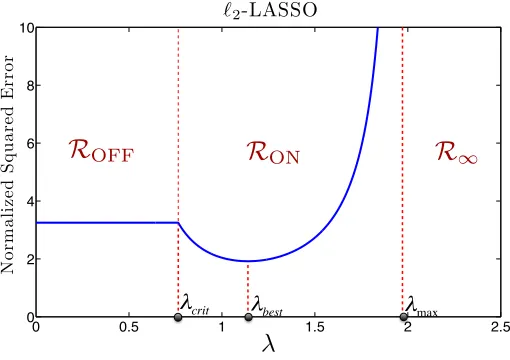
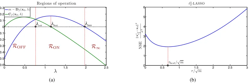
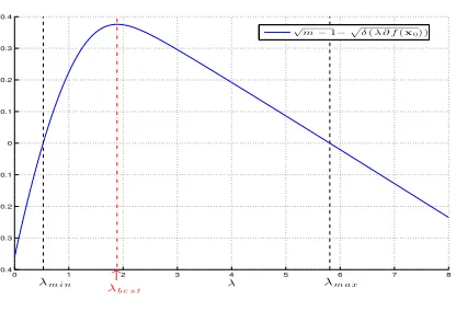
3.8 `2-LASSO: Regions of Operation . . . 92
3.9 The NSE of the`2-LASSO . . . 97
3.10 Nonasymptotic results on`2-LASSO . . . 102
3.11 Proof of Theorem 3.7 . . . 104
3.12 `2 2-LASSO . . . 108
3.13 Converse Results . . . 115
3.14 Numerical Results. . . 119
3.15 Future Directions . . . 122
4 Elementary equivalences in compressed sensing 125 4.1 A comparison between the Bernoulli and Gaussian ensembles . . . 125
4.2 An equivalence between the recovery conditions for sparse signals and low-rank matrices . . 133
5 Simultaneously Structured Models 147 5.1 Problem Setup. . . 153
5.2 Main Results: Theorem Statements . . . 156
5.3 Measurement ensembles . . . 163
5.4 Upper bounds . . . 168
5.5 General Simultaneously Structured Model Recovery . . . 171
5.6 Proofs for Section 5.2.2 . . . 178
5.7 Numerical Experiments . . . 182
5.8 Discussion. . . 185
6 Graph Clustering via Low-Rank and Sparse Decomposition 188 6.1 Model . . . 191
6.2 Main Results . . . 192
6.3 Simulations . . . 196
6.4 Discussion and Conclusion . . . 197
7.2 Universality of the Phase Transitions . . . 199
7.3 Simultaneously structured signals . . . 200
7.4 Structured signal recovery beyond convexity . . . 201
Bibliography 202 A Further Proofs for Chapter 3 227 A.1 Auxiliary Results . . . 227
A.2 Proof of Proposition 2.7. . . 231
A.3 The Dual of the LASSO . . . 235
A.4 Proofs for Section 3.5 . . . 236
A.5 Deviation Analysis: Key Lemma . . . 247
A.6 Proof of Lemma 3.20 . . . 251
A.7 Explicit formulas for well-known functions . . . 256
A.8 Gaussian Width of the Widened Tangent Cone . . . 261
B Further Proofs for Chapter 5 264 B.1 Properties of Cones . . . 264
B.2 Norms in Sparse and Low-rank Model . . . 266
B.3 Results on non-convex recovery . . . 268
C Further Proofs for Chapter 6 270 C.1 On the success of the simple program . . . 270
C.2 On the failure of the simple program . . . 285
Chapter 1
Introduction
The amount of data that is being generated, measured, and stored has been increasing exponentially in recent years. As a result, there is a growing interest in taking advantage of possible patterns and structures in the data so as to extract the desired information and overcome thecurse of dimensionality. In a wide range of applications, including computer vision, machine learning, medical imaging, and social networks, the signal that gives rise to the observations can be modeled to be approximately sparse. This has led to an immense interest in the problem of efficiently reconstructing a sparse signal from limited linear measurements, which is known as the compressed sensing (CS) problem [42,43,45,73]. Exploiting sparsity can be extremely beneficial. For instance, MRI acquisition can be done faster with better spatial resolution with CS algorithms [140]. For image acquisition, the benefits of sparsity go beyond MRI thanks to applications such as the “single pixel camera” [11].
1.1
Sparse signal estimation
Sparse approximation aims to represent a signalxas a linear combination of a few elements from a given dictionaryΨ∈Rn×d. In particular, we can writex=Ψα, whereα has few nonzero entries. Ψdepends on
the application, for instance; one can use wavelets for natural images. The aim is to parsimoniously represent xand take advantage of this representation when the time comes. The typical problem in compressed sensing assumes the linear observations ofxof the form
y=Ax+z.
HereA∈Rm×nis the measurement matrix and zis the additive noise (statisticians would use the notation y=Xβ+z). Depending on the application,A can be enforced by the problem or it can be up to us to design. To simplify the discussion, we will discard Ψ (or assume it to be identity) with the change of
variableAΨ→Aandα →x. AssumingAis full-rank, the problem is rather trivial whenm≥n, as we can estimatexwith the pseudo-inverse ofA. However,
• In a growing list of applications, the signalxis high-dimensional and the amount of observationsm may be significantly smaller thann.
• If we do know that the true signal is approximately sparse, we need a way of encouraging sparsity in our solution even in the overdetermined regimem≥n.
In the noiseless setup (z=0), to findx, we can enforcey=Ax0while trying to minimize the number of nonzero entries of the candidate solutionx0
minkx0k0 subject to Ax0=Ax.
The challenge in this formulation, especially in them<nregime, is the fact that the sparse structure we would like to enforce is combinatorial and often requires exponential search. Assumingxhasknonzero entries, xlies on one of the nk k-dimensional subspaces induced by the locations of its nonzero entries. xcan be possibly found by trying out each of them×ksubmatrices ofA; however, this method becomes exponentially difficult with increasingnandk.
Chen [58,59]. Perhaps the most well-known technique is to replace the cardinality function with the`1
norm of the signal, i.e., the sum of the absolute values of the entries. This takes us from a combinatorially challenging problem to a tractable one which can be solved in polynomial time. Moving from`0quasi-norm
to`1norm as the objective is known as “convex relaxation”. The new problem is known as the Basis Pursuit (BP) and is given as [58,59]
minkx0k1 subject to Ax0=Ax (1.1)
As it will be discussed further in Section1.2.1, convex relaxation techniques are not limited to sparse recov-ery. Important signal classes that admit low-dimensional representation allow for convex relaxation.
In general, compressed sensing and sparse approximation techniques aim to provide efficient ways to deal with the original combinatorial problem and reliably estimatex in the underdetermined regimem<
n. From a theoretical point of view, our aim is to understand the extent to which the data (x) can be undersampled while allowing for efficient reconstruction. We will often try to answer the following question:
Question 1 How many observations m do we need to reliably and efficiently estimatex?
Preferably, the answer should depend onx, only through the problem parameterskandn. The answer is also highly dependent on the specific algorithm we are using. It should be noted that the computational efficiency is another important concern and there is often a tradeoff between the computational efficiency and the estimation performance of the associated algorithm [49].
To address Question 1, since the late 1990’s there has been significant efforts in understanding the performance of sparse approximation algorithms. In 2001, Donoho and Huo provided the initial results on the recovery of a sparse signal from linear observations via BP [79]. Tropp jointly studied orthogonal matching pursuit and BP and found conditions onAfor which both both approaches can recover a sparse signal [203].
In practice, BP often performs much better than the theoretical guarantees of these initial works. Later on, it was revealed that with the help of randomness (overA), one can show significantly stronger results for BP. For instance, whenAis obtained by pickingmrows of the Discrete Fourier Transform matrix uniformly at random, it has been shown that signals up to Ologmn sparsity can be recovered via BP1. This is in fact the celebrated result of Candes, Tao, and Romberg that started CS as a field [43]. To see why this is 1We remark that Gilbert et al. also considered reconstruction of signals that are sparse in frequency domain using sublinear time
remarkable, observe thatmgrows almost linearly in the sparsitykand it can be significantly smaller than the ambient dimensionn. We should remark that no algorithm can require less thankmeasurements. We will expand more on the critical role of randomness in CS. The measurement ensembles for which we have strong theoretical guarantees (i.e. linear scaling in sparsity) are mostly random. For instance, an important class of measurement ensembles for which BP provably works are the matrices with independent and identically distributed entries (under certain tail/moment conditions) [45,73].
1.1.1 Overview of recovery conditions
In general, conditions for sparse recovery ask for A to be well-behaved and are often related with each other. In linear regression, well-behaved often means thatAis well-conditioned. In other words, denoting maximum singular value by σmax(A) and minimum singular value by σmin(A), we require σσmaxmin((AA)) to be
small. For sparse approximation, in the more interesting regimemn, we haveσmin(A) =0, hence, one
needs to look for other conditions. Some of the conditions that guarantee success of BP are as follows. •Restricted Isometry Property (RIP) [32,45]: This condition asks for submatrices ofAto be well-conditioned. Let 1≤s≤nbe an integer. Then,Asatisfies the RIP with restricted isometry constantδs, if for allm×s
submatricesAsofA, one has,
(1−δs)kvk22≤ kAsvk22≤(1+δs)kvk22
Observe that this is a natural generalization of conditioning of a matrix in the standard linear regression setup. When the system is overdetermined, settingn=s, δs characterizes the relation between minimum
and maximum singular values ofA. When RIP holds withδ2k≈0.453, it is known that BP will successfully
get back tok-sparsex. RIP is alternatively known as the uniform uncertainty principle [46].
•Incoherence [79,203]: This asks for columns ofAto have low correlation with each other. In particular, the coherence of the matrixA captures the maximum correlation between any two columns of A and is defined as follows:
µA=max
i6=j
A{i},A{j}
kA{i}k2kA{j}k2 .
Unlike the restricted isometry constant, µAcan be easily calculated. However, the type of guarantees are
later works [41,205] show that, almost linear scaling can be achieved by introducing randomness to the sparsity pattern of the signal.
•Null-Space Property (NSP) [74,85]: NSP is a condition on the null space ofA. A typical version is the following.
Definition 1.1 Asatisfies the`1-NSP of order k; if all nonzerowthat satisfiesAw=0, also satisfieskwk1>
2kwkk
1. Here, wk is the k sparse approximation ofwobtained by setting all entries0except the largest k
(in absolute value).
RIP and incoherence based conditions are often sufficient but not necessary for BP. Unlike these, NSP is “if and only if” (see Proposition1.1). IfAsatisfies`1-NSP, BP can recover anyk-sparsex; conversely, if NSP does not hold, there exists aksparse signal for which BP fails. Consequently, careful analysis of NSP can lead us to understand the exact characteristics of BP. The first such analysis is due to Donoho and Tanner who developed precise undersampling theorems whenAhas independent standard normal entries [83]. Proposition 1.1 ( [96]) SupposeA satisfies `1-NSP of order k. Then, (1.1) can recover any k sparse x.
Conversely, ifAdoes not satisfy`1-NSP, there exists a k-sparsex, for which(1.1)fails.
Proof: Letxbe ak-sparse vector and supposex∗is the minimizer of (1.1). Then,w=x∗−x∈Null(A). LetSbe a subset of{1,2, . . . ,n}be the set of nonzero locations (support) ofx. We will use the fact that, for i∈S,|xi+wi| ≥ |xi| − |wi|. It follows that
0≥ kx∗k1− kxk1≥
∑
i∈S
(|xi+wi| − |xi|)−
∑
i6∈S|wi| ≥
∑
i6∈S|wi| −
∑
i∈S|wi|.
Observe that∑i6∈S|wi|−∑i∈S|wi|=kwk1−2∑i∈S|wi| ≥ kwk1−2kwkk1>0 for all nonzerow. This implies
w=0. Conversely, if a nonzero w∈Null(A) satisfies, kwk1≤2kwkk1. Then, choosex to be−wk and
observe thatkx+wk1≤ kxk1andxis not the unique minimizer.
1.2
Low-dimensional representation via convex optimization
1.2.1 Examples of Structured Signals
•Block sparse signals and`1,2 minimization: Block sparsity [91,147,174,175,195,204,208] is a
gen-eralization of sparsity in which nonzero entries appear in blocks. One of the first work on such signals is by Rao and Kreutz-Delgado in 1999 [174] (also see [56,204,208] for earlier works). Assumen=bt for some positive integers b andt. Given x∈Rn, partition its entries intot vectors {xi}ti=1 ∈Rb such that x= [x1x2 . . . xt]T. xis called a block sparse signal if only a few of its blocks are nonzero. The “structure
exploiting” function is the`1,2norm, which is given as
kxk1,2=
t
∑
i=1kxik2.
Observe that, the`1norm is a special case of the`1,2norm where the block lengthdis equal to 1.
• Sparse representation over a dictionary: As we have mentioned previously, often the signalx is not sparse but it has a sparse representationα over a known dictionaryΨ[34,75,89]. In this case, to estimate
the signal from compressed observations one can use
ˆ
α=arg min α0 k
α0k1 subject to Ax=AΨα0, (1.2)
and let ˆx=Ψαˆ. There are several alternatives to (1.2) (see [34,211]). We remark that, often, instead of recovery from linear observationsAx, we are simply interested in finding a sparse representation given the signalx. Properties ofΨplays a critical role in the recoverability ofα andx. A related topic is learning a dictionary to sparsely represent a group of signals, which is an active research area by itself [88,141]. •Low rank matrices and nuclear norm minimization:In this case, our signal is a low-rank matrixX∈ Rd1×d2. In order to exploit the low rank structure, one can use the nuclear norm heuristic [39,40,94,128,178].
This is convex relaxation of the rank function. Denoting the i’th largest singular value of a matrixX by σi(X), its nuclear norm is denoted bykXk?and is given as follows
kXk?=
min{d1,d2}
∑
i=1σi(X).
•Discrete total variation:In many imaging applications [26,160,231] the signal of interestxrarely changes as a function of the coordinates. Consequently, lettingdi=xi+1−xifor 1≤i≤n−1, the difference vector
namely,
kxkTV =kdk1. (1.3)
•Nonuniformly sparse signals and weighted `1minimization: Sometimes, we might have prior
infor-mation regarding the sparsity pattern of the signal [48,127,165,212]. In particular, the signalxmight be relatively sparser over a certain region and denser over another. To exploit this additional information, we can use a modified`1 minimization where different weights are assigned to different regions. More rig-orously, assume that the set of entries{1,2, . . . ,n}is divided intot disjoint setsS1, . . . ,St that correspond
to regions with different sparsity levels. Then, given a nonnegative weight vectorw= [w1 w2. . . wt], the
weighted`1norm is given as
kxkw= t
∑
i=1wi
∑
j∈Si|xj|.
•Other examples:Low-rank plus sparse matrices (see Section1.2.3); simultaneously sparse and low-rank matrices, low-rank tensors (see Chapter5); sparse inverse covariance in graphical models [102]; incorporat-ing convex constraints (e.g., nonnegativity,`∞-norm, positive semidefiniteness [84,126]).
1.2.2 Generalized Basis Pursuit
These examples suggest that the success of the `1 minimization is not an isolated case, and the power of
convex relaxation is a commonly accepted phenomenon. A natural question is whether one needs to study these problems individually, or there is a general line of attack to such problems. If we focus our attention to the linear inverse problems, we can consider the generalized basis pursuit (GBP),
min
x0 f(x
0) subject to Ax0=Ax. (1.4)
The following lemma gives an equivalent of Proposition1.1for (1.4).
Proposition 1.2 xis the unique minimizer of (1.4)if and only ifNull(A)∩Df(x) ={0}.
Proof: Null(A)∩Df(x) ={0}andx∗is the minimizer. Letx∗−x=w. Ifw6=0,w6∈Df(x); which
implies f(x∗) = f(x+w)> f(x) and contradicts with the optimality ofx∗. Conversely, if there exists a nonzerow∈Null(A)∩Df(x), we have f(x+w)≤ f(x).
Proposition1.2shows that the descent setDf(x), and the null space Null(A)determine the fate of (1.4). In
Chapter2, we will see that Karush-Kuhn-Tucker optimality conditions will provide an alternative condition which is dual to NSP. It will be more convenient to study NSP in terms of the tangent cone of f(·)atx. Definition 1.3 (Tangent cone) Tangent cone is denoted byTf(x) and is obtained by taking the closure of
conic hull ofDf(x)(see Chapter2).
Clearly, Null(A)∩Tf(x) ={0} =⇒ Null(A)∩Df(x) ={0}. We next introduce the restricted singular
value of a matrix.
Definition 1.4 (Restricted singular value (RSV)) Let S be a cone inRnand letA∈Rm×n. The minimum and maximum restricted singular values ofAat S are respectively defined as
σS(A) = min
v∈S,kvk2=1kAvk2,ΣS(A) =v∈Smax,kvk2=1kAvk2.
It should be noted that similar definitions exist in the literature [50,129,206]. For instance, observe that the restricted isometry constant defined in Section1.1.1can be connected to RSV by choosing the coneSto be the set of at mosts sparse vectors. The restricted singular value provides an alternative point of view on GBP. Observe that,σTf(x)(A)>0 is equivalent to Null(A)∩Tf(x) ={0}. Hence, we have
σTf(x)(A)>0 =⇒ xis the unique minimizer of (1.4). (1.5)
On the other hand, a larger restricted singular value will imply that (1.4) is better conditioned and is more robust to noise [50].
When we have noisy observations y=Ax+z, we can consider the Basis Pursuit Denoising or lasso variation of this problem.
min
x0 λf(x
0) +1
2ky−Ax
0k2
This version tries to induce a structured signal with the help of f(·)and also tries to fit the observationsyto the estimatex0 with the second termky−Ax0k2
2. There are several questions we wish to answer regarding
these approaches.
1. How many measurements do we need to recoverxin the noiseless case? 2. What are the bounds on estimation error in the noisy setup?
3. Are there simple and intuitive quantities capturing the behavior of these problems? 4. Is there a systematic way to construct convex f(·)given the signal structure?
5. Is there a gap between what can be done in theory and the performance of the relaxed approaches? These questions have recently been subject of considerable interest. One of our main contributions will be a comprehensive answer to the second and third questions. In general, it is difficult to find answers that work for all measurement ensembles. As we seek better guarantees, we need to sacrifice the generality of the results. For instance, most results in CS requireAto be randomly generated. The sharp guarantees we obtain in Chapter3will requireAto be i.i.d. Gaussian.
1.2.3 Demixing problems
Most of our attention will focus on the linear inverse problem (1.4). However, we shall now introduce the closely related demixing problem, which will be important for Chapter 6. In demixing, we often get to observe the true signal x; however, the signal originates from a linear combination of several structured signals. The task is to identify these components.
Example: Robust principal component analysis. Suppose the matrix of interestXcan be decomposed into a low rank pieceLand a sparse pieceS, and hence it is a “mixture” of the low rank and sparse structures. This model is useful in applications such as video surveillance and face recognition [36,171,235]. The task is to splitXinto its sparse and low-rank components. OftenSis a dense sparse corruption on the desirable dataL, hence the name robust PCA. To decomposeX, the natural optimization we wish to carry out has the form
{Lˆ,Sˆ}=arg inf
L0+S0=Xrank(L
Cand`es et al. and Chandrasekaran et al. independently proposed relaxing both objectives to end up with the infimal convolution of the`1norm and the nuclear norm, [36,51]
{Lˆ,Sˆ}=arg inf
L0+S0=XkL
0k
?+γkS0k1. (1.7)
The optimization on the right hand side simultaneously emphasizes sparse and low rank pieces in the given matrix. In Chapter6, we will cast the graph clustering problem as a low-rank and sparse decomposition problem and propose convex approaches based on (1.7). The performance analysis of (1.7) focuses on the allowable levels of rank(L0)andkS0k0for which (1.7) succeeds in identifying the individual components.
The other major example is the morphological component analysis (see Elad et al. [90]). In this case, the signal is a linear combination of signals that are sparse in different basis.x=Ψ1α1+Ψ2α2. In this case,
we can minimize
{αˆ1,αˆ2}=arg min Ψ1α10+Ψ2α20=xkα
0
1k1+γkα20k1. (1.8)
In a separate line of work, McCoy and Tropp proposed a general formulation for demixing problems in a similar manner to (1.4) [144,145]. In particular, they studied the case where one of the components is multiplied by a random unitary matrix. This formulation allowed them to obtain sharper bounds compared to the related literature that deals with more stringent conditions [36,90,235].
The tools to study the convexified demixing problems (1.7) and (1.8) often parallel those of linear inverse problems. For instance, subgradient calculus plays an important role in both problems. Consequently, joint analysis of both problems appear in several works [4,36,133,221].
1.3
Phase Transitions
Returning to the basis pursuit problem (1.4), we can ask a stronger and more specific version of Question1.
Question 2 What is the exact tradeoff between sparsity and measurements to recoverxvia(1.1)?
k/p
(sparsity)
n/
p
!
1Success Phase Transition
0 0.1 0.2 0.3 0.4 0.5 0.6 0.7 0.8 0.9 1
0 0.1 0.2 0.3 0.4 0.5 0.6 0.7 0.8 0.9 1
k/n
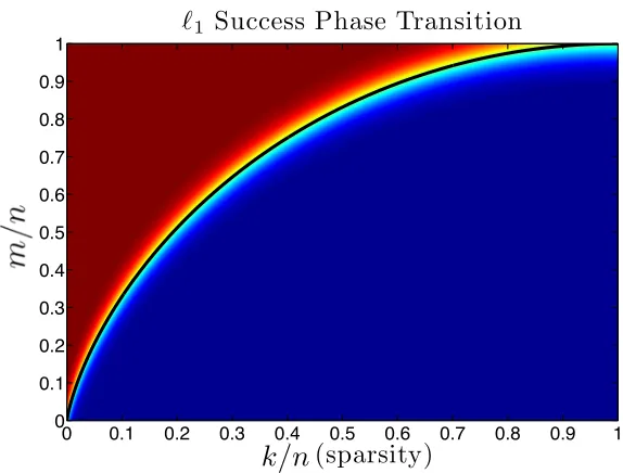
Figure 1.1: They-axis is the normalized number of measurements. x-axis is the normalized sparsity. The gradient
illustrates the gradual increase in the success of BP. As there are more measurements per sparsity (towards the red region), the likelihood of success increases. The black line is the Donoho-Tanner phase transition curve.
reconstruction with high probability. However, they derive the precise behavior as well, which is known as the Donoho-Tanner bound (illustrated in Figure1.1). Due to the universality phenomenon that we dis-cuss in Section1.4.5, studying properties of Gaussian matrices gives a good idea about other measurement ensembles as well.
In general, phase transition tries to capture the exact tradeoff between problem parameters and is not limited to linear inverse problems. In Chapter 3, we will investigate a stronger version of Question 2, namely, the precise error bounds for basis pursuit denoising. On the other hand, in Chapter 6, we will investigate the phase transitions of the graph clustering problem where we make use of convex relaxation.
1.4
Literature Survey
`1minimization.
1.4.1 Sparse signal estimation and`1minimization
Sparse signals show up in a variety of applications, and their properties have drawn attention since the 1990’s. Donoho and Johnstone used `1 regularization on wavelet coefficients in the context of function
estimation [80]. Closer to our interests, the lasso was introduced by Tibshirani [201] in 1994 as a noise robust version of (1.1). The original formulation was
min
x ky−Axk2 subject to kxk1≤τ.
whereτ ≥0 is a tuning parameter. At the same time, Donoho and Chen studied BP from a sparse signal representation perspective, whereAis a dictionary and the aim is to representyas a linear combination of few elements (columns ofA) [58,59,79]. We should remark that “orthogonal matching pursuit” is a greedy algorithm and has been extensively studied as an alternative technique [203,207].
With the introduction of compressed sensing, randomness started playing a critical role in theoretical guarantees. While guarantees for deterministic matrices requirem≥O k2, for reasonable random mea-surement ensembles one requiresm≥O(klogn). First such result is due to Candes, Tao, and Romberg [43]. They considered randomly subsampling the rows of the Discrete Fourier Transform matrix, and have shown that sparse signals can be recovered from incomplete frequencies. Later results included guarantees for ma-trices with i.i.d entries [42,45,73]. Today, state of the art results make even weaker assumptions which cover a wide range of measurement ensembles. As a generalization of sparsity, block-sparsity and non-uniform sparsity have been studied in detail [48,91,127,195]. We should emphasize that the literature on sparse recovery is vast and we only attempt to cover a small but relevant portion of it here.
1.4.2 Phase transitions of sparse estimation
Recovery types: Question2is interested in so-called weak-recovery, as we are interested in a recovery of a particular vector x. There is also the notion of strong recovery, which asks for the same (random) measurement matrix to recover allk-sparse vectors via BP. Observe that, Proposition1.1gives the condition for the strong recovery. Clearly, strong recovery will require more measurements for the same sparsity level compared to the weak recovery.
Neighborly polytopes: As we discussed in the previous section, Donoho and Tanner found upper bounds on the required number of samples by studying neighborly polytopes and grassman angle com-putations. They show that their bounds are tight in the regime where the relative sparsity kn tends to zero. Remarkably, these upper bounds were observed to be tight in simulation for all sparsity regimes [74,83,85]. The fact that the Donoho-Tanner bound is apparently tight gained considerable attention. As follow-up works Xu, Khajehnejad, and Hassibi studied several variations of the phase transition problem by extending the Grassman Angle approach. In [225,226], they showed that whenmis above the bound, BP also enjoys robustness when recovering approximately sparse signals. In [127,224,227] they have analyzed weighted and reweighted`1minimization algorithms, and have provably shown that such algorithms could allow one
to go beyond the Donoho-Tanner bound.
Gaussian comparison inequalities: In 2008, Versynin and Rudelson used Gaussian comparison in-equalities to study BP [184]. They found≈8klognk measurements to be sufficient with a short argument. This is strikingly close to the optimal closed form bound 2klognk. Later on, Stojnic carried out a more careful analysis of comparison inequalities to obtain better bounds for`1minimization [192]. Remarkably, Stojnic’s
analysis was able to recover the Donoho-Tanner bound with a more generalizable technique (compared to Grassman angle), which can be extended to other structured signal classes. The tightness of Donoho-Tanner bound has been proven by Amelunxen et al. [4], as well as Stojnic [194]. Namely, they show that, below the Donoho-Tanner bound, BP will fail with high probability (also see Section1.4.4).
1.4.3 Low-rank estimation
The abundance of strong theoretical results on sparse estimation led researchers to consider other low-dimensional representation problems. Low-rank matrices show up in a variety of applications and they resemble sparse signals to a good degree. The rank minimization problem has first been considered in low-order control system design problems [95,178]. Convex relaxation for the rank minimization (RM) problem is due to Fazel, who replaced rank function with nuclear norm and also cast it as a semidefinite program [94]. Initial results on RM were limited to applications and implementations.
The significant theoretical developments in this problem came relatively later. This was made possible by advances in sparse estimation theory and similarities between sparse and low-rank recovery problems. Recht, Fazel, and Parrilo studied the RM problem from a compressed sensing point of view, where they studied the number of measurements required to recover a low-rank matrix [178]. They introduced matrix RIP and showed that it is sufficient to recover low-rank matrices via NNM. For i.i.d subgaussian measure-ments, they also show that matrix RIP holds withO(rnlogn)measurements. This is a significant result, as one needs at leastO(rn)measurements to accomplish this task (information theoretic lower bound). Candes and Plan improved their bound toO(rn), which is information theoretically optimal [39].
Another major theoretical development on RM came with results on matrix completion (MC). Low-rank matrix completion is a special case of the rank minimization problem. In MC, we get to observe the entries of the true matrix, which we believe to be low-rank. Hence, measurement model is simpler compared to i.i.d measurements obtained by linear combinations of the entries weighted by independent random variables. This measurement model also has more applications, particularly in image processing and recommendation systems. Results on MC requires certain incoherence conditions on the underlying matrix. Basically, the matrix should not be spiky and the energy should be distributed smoothly over the entries. The first result on MC is due to Candes and Recht [40], who show thatO r2n·polylog(n)
measurements are sufficient for MC via nuclear norm minimization. There is a significant amount of theory dedicated to improving this result [37,60,125,128]. In particular, the current best known results requireO rnlog2n, where the theoretical lower bound isO(rnlogn)[47,177].
measurements are sufficient to guarantee low-rank recovery via NNM. Chandrasekaran et al. have similar results, which will be discussed next [50].
1.4.4 General approaches
The abundance of results on the estimation of structured signals naturally led to the development of a unified understanding of these problems. Focusing on the linear inverse problems, we can tackle the generalized basis pursuit,
minf(x0) subject to Ax0=Ax. (1.9)
This problem has recently been a popular topic. The aim is to develop a theory for the general problem and recover specific results as an application of the general framework. A notable idea in this direction is the atomic norms, which are functions that aim to parsimoniously represent the signal as a sum of a few core signals called “atoms”. For instance, ifx is sparse over the dictionaryΨ, the columns ofΨ will be the corresponding atoms. This idea goes back to mid 1990’s where it appears in the approximation theory literature [68]. Closer to our discussion, importance of minimizing these functions, is first recognized by Donoho in the context of Basis Pursuit [58]. More recently, in connection to atomic norms, Chandrasekaran et al. [50] analyze the generalized basis pursuit with i.i.d Gaussian measurements using Gaussian compar-ison results. They generalize the earlier results of Vershynin, Rudelson and Stojnic [184,192] (who used similar techniques to study BP) and find upper bounds to the phase transitions of GBP, which are seemingly tight. Compared to the neighborly polytopes analysis of [74,83,224], Gaussian comparison inequalities re-sult in more geometric and intuitive rere-sults; in particular, “Gaussian width” naturally comes up as a way to capture the behavior of the problem (1.9). While the Gaussian width was introduced in 1980’s [111,112], its importance in compressed sensing is discovered more recently by Vershynin and Rudelson [184]. Gaussian width is also important for our exposition in Section1.5, hence we will describe how it shows up in (1.9). Definition 1.5 (Gaussian width) Letg∈Rnbe a vector with independent standard normal entries. Given a set S⊂Rn, its Gaussian width is denoted byω(S)and is defined as
ω(S) =E[sup
v∈S
vTg].
values of Gaussian matrices.
Proposition 1.3 Denote the unit`2-ball byBn−1. Suppose S is a cone inRn. LetG∈Rm×nhave indepen-dent standard normal entries. Then, with probability1−exp(−t2
2)
σS(G)≥
√
m−1−ω(S∩Bn−1)−t.
This result is first used by Rudelson and Vershynin for basis pursuit [184]. Further developments in this direction are due to Mendelson et al. [151,153]. Chandrasekaran et al. have observed that this result can be used to establish success of the more general problem GBP. In particular, combining (1.5) and Proposition
1.3ensures that, ifm≥(ω(Tf(x)∩Bn−1) +t)2+1, GBP will succeed with high probability. Stojnic was
the first person to do a careful and tight analysis of this for basis pursuit and to show that Donoho-Tanner phase transition bound is in fact equal toω(T`1(x)∩B
n−1)2[192].
The Gaussian width has been subject of several follow-up works, as it provides an easy way to analyze the linear inverse problems [4,18,49,163,165,175]. In particularω(Tf(x)∩Bn−1)2has been established
as an upper bound on the minimum number of measurements to ensure success of GBP. Remarkably, this bound was observed to be tight in simulation, in other words, whenm<ω(Tf(x)∩Bn−1)2, GBP would
fail with high probability.
It was proven to be tight more recently by Amelunxen et al. [4]. Amelunxen et al.’s study is based on the intrinsic volumes of convex cones, and their results are applicable in demixing problems as well as linear inverse problems. Stojnic’s lower bound is based on a duality argument; however, he still makes use of comparison inequalities as his main tool [194].
1.4.5 Universality of the phase transitions
Donoho-Tanner type bounds are initially proven only for Gaussian measurements. However, in simula-tion, it is widely observed that the phase transition points of different measurement ensembles match [71]. Examples include,
• Matrices with i.i.d subgaussian entries
While this is a widely accepted phenomenon, theoretical results are rather weak. Bayati et al. recently showed the universality of phase transitions for BP via connection to the message passing algorithms for i.i.d subgaussian ensembles [12]2. Universality phenomenon is also observed in the general problem (1.4); however, we are not aware of a significant result on this. For GBP, the recent work by Tropp shows that, subgaussian measurements have similar behavior to Gaussian ensemble up to an unknown constant over-sampling factor [206] (also see works by Mendelson et al. [129,152] and Ai et al. [2]). In Chapter4.1, we investigate the special case of Bernoulli measurement ensemble, where we provide a short argument that states that 7ω(Tf(x)∩Bn−1)2Bernoulli measurements are sufficient for the success of GBP.
1.4.6 Noise Analysis
One of the desirable properties of an optimization algorithm is stability to perturbations. The noisy estima-tion of structured signals has been studied extensively in the recent years. In this case, we get to observe corrupted linear observations of the formy=Ax+z. Let us call the recovery stable if the estimate ˆxsatisfies kxˆ−xk2≤Ckzk2for a positive constantC.
Results on sparse estimation: In case of`1 minimization, most conditions that ensure recovery of a
sparse signal from noiseless observations also ensure stable recovery from noisy observations (e.g., RIP, NSP). Both the lasso estimator (1.6) and the Dantzig selector do a good job at emphasizing a sparse solution while suppressing the noise [19,31,201]. For related literature see [19,31,45]. There is often a distinction between worst-case noise analysis and the average-case noise analysis.
Assume A has i.i.d standard normal entries with variance m1 and m≥O klog2kn. It can be shown that, with high probability, kxˆ−xk2≤Ckzk2 for a positive constant for all vectorsz[32,43,45,50,225].
This includes the adversarial noise scenario wherezcan be arranged (as a function ofA,x) to degrade the performance. On the other hand, the average-case reconstruction errorkxˆ−xk22 (zis independent ofA) is known to scale asO
klogn
m kzk
2 2
[19,31,33,82,172]. In this case,zdoes not have the knowledge ofAand is not allowed to be adversarial.
Average-case noise is what we face in practice and it is an attractive problem to study. The exact error behavior has been studied by Donoho, Maleki, and Montanari [13,82] in connection to the Approximate Message Passing framework. They are able to find the true error formulas (so-called the noise-sensitivity bounds) which hold in high dimensions, as a function of the sparsityk,m, and the signal-to-noise ratio. 2They have several other constraints. For instance, the results are true asymptotically inm,n,k. They also require that the
Results on the generalized basis pursuit: For the general problem, Chandrasekaran et al. have worst-case error bounds, which follows from arguments very similar to the noiseless worst-case [50]. Negahban et al. provide order-optimal convergence rates under a “decomposability” assumption on f [161]. The average-case analysis for arbitrary convex functions and sharp error bounds with correct constants are studied by Oymak et al. in [170,200] and they are among the contributions of this dissertation.
1.4.7 Low-rank plus sparse decomposition
In several applications, the signalXcan be modeled as the superposition of a low-rank matrixLand a sparse matrixS. From both theory and application motivated reasons, it is important to understand under what conditions we can splitXintoLandS, and whether it can be done in an efficient manner. The initial work on this problem is due to Chandrasekaran et al. where authors derived deterministic conditions under which (1.7) works [51]. These conditions are based on the incoherence between the low-rank and the sparse signal domains. In particular we require the low-rank column-row spaces to not be spiky (diffused entries), and the support of the sparse component to have a diffused singular value spectrum. Independently, Cand`es et al. studied the problem in a randomized setup where the nonzero support of the sparse component is chosen uniformly at random. Similar to the discussion in Section 1.1, randomness results in better guarantees in terms of the sparsity-rank tradeoff [36]. The problem is also related to the low-rank matrix completion, where we observe few entries of a low-rank matrix corrupted by additive sparse noise [1,36,235]. In Chapter
6, we propose a similar problem formulation for the graph clustering problem.
1.5
Contributions
k/p
n/
p
Lasso Error Heatmap
0 0.1 0.2 0.3 0.4 0.5 0.6 0.7 0.8 0.9 1
0 0.1 0.2 0.3 0.4 0.5 0.6 0.7 0.8 0.9 1 1.1 1.2 1.3 1.4 1.5
m n
k/n
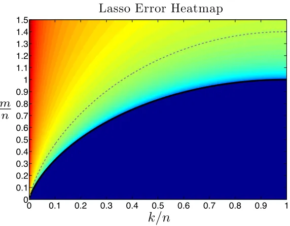
Figure 1.2:We plot (1.11) for sparse recovery. The black line is the Donoho-Tanner bound; above which the recovery
is robust. The warmer colors correspond to better reconstruction guarantees; hence, this figure adds an extra dimension
to Figure1.1; which only reflects “success” and “failure”. Dashed line corresponds to the fixed reconstruction error.
Remark: The heatmap is clipped to enhance the view (due to singularities of (1.11)).
1.5.1 A General Theory of Noisy Linear Inverse Problems
In Chapter3, we consider the noisy systemy=Ax+z. We are interested in estimatingxand the normalized estimation errorNSE = Ekxˆ−xk22
Ekzk22
when A∈Rm×n has independent standard normal entries. Whenm>n, the standard approach to solve this overdetermined system of equations is the least squares method. This method is credited to Legendre and Gauss and is approximately 200 years old. The estimate is given by the pseudo-inverse ˆx= (AAT)−1ATyand it can be shown that the error is approximately n
m−n, wherem−n
corresponds to the statistical degrees of freedom (here the difference between the number of equations and the number of unknowns). When the system is underdetermined (m<n), as is the case in many applications, the problem is ill-posed and unique reconstruction is not possible in general. Assuming that the signal has a structure, the standard way to overcome this challenge is to use the lasso formulation (1.6). In Chapter3, we are able to give precise error formulas as a function of,
To give an exposition to our result, let us first consider the following variation of the problem.
min
x0 ky−Ax
0k
2 subject to f(x0)≤ f(x) (1.10)
We prove that the NSE satisfies (with high probability),
Ekxˆ−xk22
Ekzk22 .
ω(Tf(x)∩Bn−1)2
m−ω(Tf(x)∩Bn−1)2
. (1.11)
Furthermore, the equality is achieved when signal-to-noise ratio kxk22
E[kzk2 2]
approaches∞. We also show that,
this is the best possible bound that is based on the knowledge of the first order statistics of the function. Here, first order statistics means knowledge of the subgradients atx, and will become clear in Chapter3.
From Section1.4.4, recall thatω(Tf(x)∩Bn−1)2is the quantity that characterizes the fate of the
noise-less problem (1.4). Whenxis ak-sparse vector and we use`1optimization, (1.11) reduces to the best known
error bounds for sparse recovery, namely,
Ekxˆ−xk22 Ekzk22
. 2klog
n k
m−2klognk.
This particular bound was previously studied by Donoho, Maleki, and Montanari under the name “noise sensitivity” [13,82]. (1.11) has several unifying aspects:
• We generalize the results known for noiseless linear inverse problems. Stable reconstruction is possi-ble if and only ifm>ω(Tf(x)∩Bn−1)2.
• Setting f(·) =0 reduces our results to standard least-squares technique whereω(Tf(x)∩Bn−1)2=n.
Hence, we recover the classic result mn−n.
• We provide a generic guarantee for structured recovery problems. Instead of dealing with specific cases such as sparse signals, low-rank matrices, block-sparsity, etc, we are able to handle any abstract norm, and hence treat these specific cases systematically.
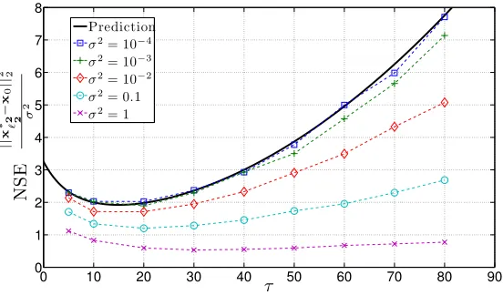
Penalized problems: (1.10) requires information about the true signal, namely, f(x). The more useful formulation (1.6) uses penalization instead. In Chapter3, we also study (1.6) as well as its variation,
min
x0 ky−Ax
0k
2+λf(x0). (1.12)
of Gaussian width. We show that the error bounds for (1.12) are captured by this new term, which can reflect the precise dependence onλ. In addition to error bounds, our results yield the optimal penalty parameters for (1.6) and (1.12), which can achieve the bound (1.11). We defer the detailed analysis and rigorous statements of our results to Chapter3.
1.5.2 Elementary equivalences in compressed sensing
In Chapter 4, we present two results which are relatively short and are based on short and elementary arguments. These are
• investigating properties of the Bernoulli measurement ensemble via connection to Gaussian ensemble, • investigating RIP conditions for low-rank recovery via connection to RIP of sparse recovery.
1.5.2.1 Relating the Bernoulli and Gaussian ensembles
So far, we have discussed the importance of the Gaussian ensemble. In particular, one can find the exact performance when the sensing matrix has independentN(0,1)entries. We have also discussed the univer-sality phenomenon which is partially solved for`1-minimization. In Chapter4.1, we consider (1.4) when Ahas symmetric Bernoulli entries which are equally likely to be±1. To analyze this, we write a Gaussian matrixGas,
G=
r 2
πsign(G) +R
where sign(·)returns the element-wise signs of the matrix, i.e.+1 ifGi,j≥0 and−1 else. Observe that, this
decomposition ensures sign(G)is identical to a symmetric Bernoulli matrix. Furthermore,Ris a zero-mean matrix conditioned on sign(G). Based on this decomposition, we show that,
m≈7ω(Tf(x0)∩Bn−1)2
Bernoulli samples are sufficient for successful recovery. Compared to the related works [2,152,206], our argument is concise and yields reasonably small constants. We also find a deterministic relation between the restricted isometry constants and restricted singular values of Gaussian and Bernoulli matrices. In particular, restricted isometry constant corresponding to a Bernoulli matrix is at most π
m/d2
r
d
/
m
0 0.1 0.2 0.3 0.4 0.5 0.6 0.7 0.8 0.9 1
0 0.1 0.2 0.3 0.4 0.5 0.6 0.7 0.8 0.9 1
Weak bound Strong bound
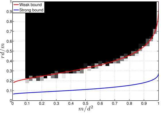
Figure 1.3: To illustrate the linear growth of the phase transition point inrd, we chose they-axis to be rdm and the
x-axis to be the normalized measurements m
d2. Observe that only weak bound can be simulated and it shows a good
match with simulations. The numerical simulations are done for a 40×40 matrix and whenm≥0.1d2. The dark
region implies that (1.13) failed to recoverX.
1.5.2.2 Relating the recovery conditions for low-rank and sparse recovery
1.5.2.3 Phase transitions for nuclear norm minimization
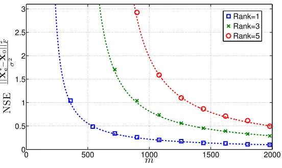
Related to Section1.5.2.2and as mentioned in Section1.4.3, in [163,165] we study the sample complexity of the low-rank matrix estimation via nuclear norm minimization3. In particular, given a rankr matrix X∈Rd×d, we are interested in recovering it fromA(X)whereA(·):Rd×d→Rmis a linear i.i.d Gaussian map, i.e. A(X)is equivalent to castingXinto ad2×1 vector and multiplying with anm×d2 matrix with independent standard normal entries. We consider
arg min
X0 kX
0k
? subject to A(X0) =A(X) (1.13)
as the estimator. In [163], we find Donoho-Tanner type precise undersampling bounds for this problem (il-lustrated in Figure1.3). As mentioned in Section1.4.2, the weak bound asks for the recovery of a particular rank r matrix, while the strong bound asks for the recovery of all rankr matrices simultaneously by the same realization of A. We showed that whenm is above the bounds (1.13) will succeed. However, the recent progress on phase transitions strongly indicates that, our “weak threshold” is indeed tight [4,77,194]. In [165], we provide a robustness analysis of (1.13) and also find closed-form bounds:
• To ensure weak recovery one needsm&6rdsamples. • To ensure strong recovery one needsm&16rd samples.
Considering that a rankr matrix has 2dr−r2 degrees of freedom [40], the weak bound suggests that, one needs to oversampleXby only a factor of 3 to efficiently recover it from underdetermined observations.
1.5.3 Simultaneously structured signals
Most of the attention in the research community has focused on signals that exhibit a single structure, such as variations of sparsity and low-rank matrices. However, signals exhibiting multiple low-dimensional structures do show up in certain applications. For instance, in certain applications, we wish to encourage a solution which is not only sparse but whose entries also vary slowly, i.e., the gradient of the signal is approximately sparse as well (recall (1.3)). Tibshirani proposed fused lasso optimization for this task [202],
arg minλ`1kx0k1+λTVkx0kTV+
1
2ky−Ax
0k2 2.
As a second example, we will talk about matrices that are simultaneously sparse and low-rank. Such matrices typically arise from sparse vectors, with the mappinga→A=aaT, where a is a sparse vector itself. This mapping is also known as lifting as we move from lower dimensionalRnto a higher dimensional spaceRn×n. The new variableAhas rank 1 and is also sparse. This model shows up in several applications, including sparse principal component analysis [236] and sparse phase retrieval [44,92,122].
Example: Sparse Phase Retrieval. Phase retrieval is the problem of estimating a signal from its phaseless observations. For instance, assume we get to observe power spectral density (PSD) of a signal. PSD is obtained by taking the square of the Fourier Transform and is phaseless. In certain applications, most notably X-Ray crystallography, one only has access to PSD information and the task is to find a solution to the given PSD. There are multiple signals that can yield the same power spectral density, and hence we often need an additional criteria to optimize over. This criteria is often the sparsity of the underlying signal, which yields the problem “sparse phase retrieval”. In finite dimensions, the noiseless phase retrieval problem assumes phaseless measurementsyi={|aTi x|2}
m
i=1of the true vectorx, where{ai}mi=1are the measurement
vectors. Hence, sparse PR problem is given as
kx0k0 subject to |aiTx0|2=yi.
This problem is nontrivial due to the quadratic equality constraints as well as the combinatorial objective. Applying the liftingx→X=xxT proposed by Balan et al. [9], we end up with linear measurements in the
new variableX,
kX0k0 subject to
aiaTi ,X0
=yi, rank(X0) =1, X00.
Relaxing the sparsity and rank constraints by using`1and nuclear norm, we find a convex formulation that
encourages a low-rank and sparse solution.
kX0k1+λkX0k? subject to X00,
aiaTi ,X0
=yi,1≤i≤m. (1.14)
Traditional convex formulations for the sparse PCA problem have a striking similarity to (1.14) and also make use of nuclear norm and`1norm [64].
Finally, we remark that low-rank tensors are yet another example of simultaneously structured signals [103,158] and they will be discussed in more detail in Chapter5.
perfor-mance guarantees, i.e., we don’t lose much by solving the relaxed objective compared to the true objective. For example, countless papers in literature show that`1 norm does a great job in encouraging sparsity. In (1.14), the signal has two structures, and hence it has far fewer degrees of freedom compared to an only low-rank or only sparse matrix. We investigate whether it is possible to do better (i.e., use fewer measurements) by making use of this fact. We show that the answer is negative for any cost function that combines the`1
and nuclear norms. To be more precise, by combining convex penalties, one cannot reduce the number of measurements much beyond what is needed for the best performing individual penalty (`1or nuclear norm).
In Chapter5, we will study the problem for abstract signals that have multiple structures and arrive at a more general theory that can be applied to the specific signal types.
Our results are easy to interpret and apply to a wide range of measurement ensembles. In particular, we show the limitations of standard convex relaxations for the sparse phase retrieval and the low-rank tensor completion problems. For the latter one, each observation is a randomly chosen entry of the tensor. To give a flavor of our results, let us return to the sparse and low-rank matrices, where we investigate,
kX0k1+λkX0k? subject to X00,
Gi,X0
=yi,1≤i≤m. (1.15)
For simplicity, let{Gi}mi=1be matrices with independent standard normal entries andA(·):Rn×n→Rmis the measurement operator. Suppose the true signal isX=xxT, wherex∈Rnis ak-sparse vector. To simplify the consequent notation, let us assume that the nonzero entries ofxare comparable, i.e., kkxxk1k2 ≈O√k
. Then, we have the following,
• If only`1norm is used (λ=0), CS theory requiresO k2lognk
measurements to retrieveXvia (1.15). • If only nuclear norm is used, results on rank minimization requiresO(n)measurements to retrieveX. • Our results in Chapter 5ensure that one needs at leastΩ(min{k2,n}) measurements for any choice
ofλ.
• Replace the objective function in (1.15) by kX0k0+λrank(X0). There is a suitable λ, for which
O klognkmeasurements are sufficient.
1.5.4 Convex Optimization for Graph Clustering
Our results so far focused on the study of linear inverse problems. In Chapter 6, we consider a more application-oriented problem, namely, graph clustering. Graphs are important tools to represent data effi-ciently. An important task regarding graphs is to partition the nodes into groups that are densely connected. In the simpler case, we may wish to find the largest clique in the graph, i.e., the largest group of nodes that are fully connected to each other. In a similar flavor to the sparse estimation problem, the clustering problem is challenging and highly combinatorial. Can this problem be cast in the convex optimization framework? It turns out the answer is positive. We pose the clustering problem as a demixing problem where we wish to decompose the adjacency matrix of the graph into a sparse and low-rank component. We then formulate two optimizations, one of which is tailored for sparse graphs. Remarkably, performance of convex optimization is on par with alternative state-of-the-art algorithms [6,7,146,164] (also see Chapter6). We carefully ana-lyze these formulations and obtain intuitive quantities, dubbed “effective density”, that sharply capture the performance of the proposed algorithms in terms of cluster sizes and densities.
Let the graph haven nodes, andAbe the adjacency matrix, where 1 corresponds to an edge between two nodes and 0 corresponds to no edge. Ais a symmetric matrix, and, without loss of generality, assume diagonal entries are 1. Observe that a clique corresponds to a submatrix of all 1’s. The rank of this submatrix is simply 1. With this observation, Ames and Vavasis [6] proposed to find cliques via rank minimization, and used nuclear norm as a convex surrogate of rank. We cast the clustering problem in a similar manner to the clique finding problem, where cliques can have imperfections in the form of missing edges. Assuming there are few missing edges, each cluster corresponds to the sum of a rank 1 matrix and a sparse matrix.
Let us assume the clusters are disjoint. Our first method (dubbed simple method) solves the following,
minimize
L,S kLk?+λkSk1 (1.16)
subject to
1≥Li,j≥0 for alli,j∈ {1,2, . . .n}
L+S=A.
The nuclear norm and the`1norm are used to induce a low-rankLand sparseS, respectively. The hope is thatLi,jwill be 1 whenever nodesiand jwill lie in the same cluster, and 0 otherwise. This way, rank(L)
We investigate this problem for the well-known stochastic block model [117], which is essentially a nonuniform Erd¨os-Renyi graph. While Chapter6considers a general model, let us introduce the following setup for the exposition.
Definition 1.6 (Simple Block Model) Assume thatG is a random graph with n nodes with t clusters, where
each cluster has size d. LetAbe the corresponding adjacency matrix. Further assume that the existence of
each edge is independent of each other, and
P(Ai,j=1) =
p if i,j is in the same cluster
q else
for some constants p>q>0.
Assumingd,nare large,d=o(n)andλ is well-tuned, for the simple block model, we find that, • (1.16) correctly identifies the planted clusters ifq<12 andd(2p−1)>4pq(1−q)n. • (1.16) fails ifd(2p−1)<√qnorq>1
2.
Here, d(2p−1) jointly captures the size and density of the planted clusters; hence, we call it effective density. Assumingq< 1
2,d(2p−1) is tightly sandwiched between
√qnand 4√qn. This result indicates that cluster sizes should grow with √n, which is consistent with state of the art results on clique finding [6,7,61,67,185].
The simple method has critical drawbacks, as we require p>1
2 >q. The algorithm tailored for sparse
graphs (dubbed “improved method”) is able to overcome this bottleneck. This new algorithm only requires p>qand will succeed when
d(p−q)>2pq(1−q)n.
1.5.5 Organization
In Chapter 2, we go over the mathematical notation and tools that will be crucial to our discussion throughout this dissertation.
In Chapter3, we study the error bounds for the noisy linear inverse problems. We formulate three ver-sions of the lasso optimization and find formulas that accurately capture the behavior based on the summary parameters Gaussian width and Gaussian distance.
Chapter4will involve two topics. We first analyze Bernoulli measurement ensemble via connection to the Gaussian measurement ensemble. Next, we study the low-rank approximation problem by establishing a relation between the sparse and low-rank recovery conditions.
Chapter5is dedicated to the study of simultaneously structured signals. We formulate intuitive convex relaxations for recovery of these signals and show that there is a significant gap between the performance of convex approaches and what is possible information theoretically.
In Chapter6, we develop convex relaxations for the graph clustering problem. We formulate two ap-proaches, where one is particularly tailored for sparse graphs. We find intuitive parameters based on the density and size of the clusters that sharply characterize the performance of these formulations. We also numerically show that performance is on par with more traditional algorithms.
Chapter 2
Preliminaries
We will now introduce some notation and definitions that will be used throughout the dissertation.
2.1
Notation
Vectors and matrices:Vectors will be denoted by bold lower case letters. Given a vectora∈Rn,aTwill be used to denote its transpose. For p≥1,`pnorm ofawill be denoted bykakpand is equal to(∑ni=1|ai|p)1/p.
The `0 quasi-norm returns the number of nonzero entries of the vector and will be denoted bykak0. For
a scalar a, sgn(a) returns its sign i.e. a·sgn(a) =|a|and sgn(0) =0. sgn(·):Rn→Rn returns a vector consisting of the signs of the entries of the input.
Matrices will be denoted by bold upper case letters. n×n identity matrix will be denoted byIn. For
a given matrix A∈Rn1×n2, its null space and range space will be denoted by Null(A) and Range(A),
respectively. To vectorize a matrix, we can stack its columns on top of each other to obtain the vector vec(A)∈Rn1n2. rank(A)will denote the rank of the matrix. The minimum and maximum singular values
of a matrixAare denoted byσmin(A)andσmax(A). σmax(A)is equal to the spectral normkAk. kAkF will
denote the Frobenius norm. This is essentially equivalent to the`2 norm of the vectorization of a matrix: kAk2F = (∑ni=11∑nj=21A2i,j)1/2. tr(·)will return the trace of a matrix.
Probability: We will useP(·)to denote the probability of an event. E[·]and Var[·]will be the expectation and variance operators, respectively. Gaussian random variables will play a critical role in our results. A multivariate (or scalar) normal distribution with mean µµµ ∈Rn and covarianceΣΣΣ∈Rn×n will be denoted byN (µµµ,ΣΣΣ). “Independent and identically distributed” and “with high probability” will be abbreviated as
Convex geometry: Denote the unit `2 sphere and the unit`2 ball inRn bySn−1andBn−1, respectively. dim(·) will return the dimension of a linear subspace. For convex functions, the subgradient will play a critical role.sis a subgradient of f(·)at the pointv, if for all vectorsw, we have that,
f(v+w)≥ f(v) +sTw.
The set of all subgradientssis called the subdifferential and is denoted by∂f(v). If f:Rn→Ris continuous atv, then the subdifferential∂f(v)is a convex and compact set [23]. For a vectorx∈Rn,kxk denotes a general norm andkxk∗=supkzk≤1hx,ziis the corresponding dual norm. Finally, the Lipschitz constant of
the function f(·)is a numberLso that, for allv,u, we have that,|f(v)−f(u)| ≤Lkv−uk2.
Sets:Given setsS1,S2∈Rn,S1+S2will be the Minkowski sum of these sets, i.e.,{v1+v2
v1∈S1,v2∈S2}.
Closure of a set is denoted by Cl(·). For a scalarλ ∈Rand a nonempty setS⊂Rn,λSwill be the dilated set, and is equal to{λv∈Rn v∈S}. The cone induced by the setS will be denoted by cone(S)and is equal to{λvλ ≥0, v∈S}. It can also be written as a union of dilated sets as follows,
cone(S) = [
λ≥0 λS.
The polar cone ofSis defined asS◦={v∈RnvTu≤0∀u∈S}. The dual cone isS∗=−S◦.
2.2
Projection and Distance
Given a pointvand a closed and convex setC, there is a unique pointainC satisfyinga=arg mina0∈Ckv− a0k2. This point is the projection ofvontoC and will be denoted as ProjC(v)or Proj(v,C). The distance
vector will be denoted byΠC(v) =v−ProjC(v). The distance to a set is naturally induced by the definition
of the projection. We will let distC(v) =kv−ProjC(v)k2.
WhenC is a closed and convex cone, we have the following useful identity due to Moreau [157].
Fact 2.1 (Moreau’s decomposition theorem) LetC be a closed and convex cone inRn. For anyv∈Rn, the following two are equivalent:
1. v=a+b,a∈C,b∈C◦andaTb=0.
Fact 2.2 (Properties of the projection, [17,23]) AssumeC ⊆Rnis a nonempty, closed, and convex set and a,b∈Rnare arbitrary points. Then,
• The projection Proj(a,C)is the unique vector satisfying, Proj(a,C) =arg minv∈Cka−vk2.
• hProj(a,C),a−Proj(a,C)i=sups∈Chs,a−Proj(a,C)i.
• kProj(a,C)−Proj(b,C)k2≤ ka−bk2.
Descent set and tangent cone:Given a function f(·)and a pointx, descent set is denoted byDf(x), and is
defined as
Df(x) ={w∈Rn f(x+w)≤f(x)}.
We also define the tangent cone of f atxasTf(x):=Cl(cone(Df(x))). In words, tangent cone is the
closure of the conic hull of the descent set. These concepts will be quite important in our analysis. Recall that Proposition1.2is based on the descent cone and is essentially the null-space property for the GBP. The tangent cone is related to the subdifferential∂f(x)as follows [182].
Proposition 2.1 Suppose f :Rn→Ris a convex and continuous function. The tangent cone has the follow-ing properties.
• Df(x)is a convex set andTf(x)is a closed and convex cone.
• Supposexis not a minimizer of f(·). Then,Tf(x)◦ =cone(∂f(x)).
2.2.1 Subdifferential of structure inducing functions
Let us introduce the subdifferential of the`1norm.
Proposition 2.2 ( [72]) Givenx∈Rn,s∈∂kxk1if and only if,si=sgn(xi)for all i∈supp(x)and|si| ≤1
else.
Related to this, we define the soft-thresholding (a.k.a. shrinkage) operator. Definition 2.1 (Shrinkage) Givenλ≥0, shrinkλ(·):R→Ris defined as,
shrinkλ(x) =
While the importance of shrinkage will become clear later on in the simplest setup, it shows up when one considers denoising by`1minimization [72].
Proposition 2.3 Suppose we see the noisy observations y=x+z and we wish to estimate x via xˆ =
arg min
x0 λkx
0k
1+12ky−x0k22. The solutionxˆ is given by
ˆ
xi=shrinkλ(yi) f or 1≤i≤n.
This in turn is related to the distance of a vector to the scaled subdifferential, which will play an important role in Chapter3. It follows from Proposition2.2thatΠ(v,λ ∂kxk1)i=vi−λsgn(xi)when i∈supp(xi)
and shrink(vi)wheni6∈supp(xi).
We will also discuss that subdifferentials of`1,2 norm and the nuclear norm have very similar forms to
that of`1norm, and the distance to the subdifferential can again be characterized by the shrinkage operator.
For instance, the nuclear norm is associated with shrinking the singular values of the matrix while the`1,2
norm is associated with shrinking the`2norms of the individual blocks [50,70,77].
2.3
Gaussian width, Statistical dimension and Gaussian distance
We have discussed Gaussian width (Def. 1.5) in Chapter1.4and its importance in dimension reduction via Gaussian measurements. We now introduce two related quantities that will be useful for characterizing how well one can estimate a signal by using a structure inducing convex function1. The first one is the Gaussian squared-distance.
Definition 2.2 (Gaussian squared-distance) Let S∈Rn be a subset of Rn andg∈Rn have independent N (0,1)entries. Define the Gaussian squared-distance of S to be,
D(S) =E[inf
v∈Skg−vk
2 2]
Definition 2.3 (Statistical dimension) LetC ∈Rnbe a closed and convex cone andg∈Rnhave indepen-dentN (0,1)entries. Define the statistical dimension ofC to be,
δ(C) =E[kProj(g,C)k22]
k-sparse, x0∈Rn Rankr, X0∈Rd×d k-block sparse,x0∈Rtb
δ(Tf(x0)) 2k(lognk+1) 6dr 4k(log
t k+b)
D(λ ∂f(x0)) (λ2+3)k for λ ≥
p
2 lognk λ2r+2d(r+1) for λ≥2√d (λ2+b+2)k for λ≥√b+q2 logtk
Table 2.1: Closed form upper bounds forδ(Tf(x0))( [50,101]) andD(λ ∂f(x0))corresponding to sparse,
block-sparse signals and low-rank matrices described in Section1.2.1. See SectionA.7for the proofs.
The next proposition provides some basic relations between these quantities.
Proposition 2.4 Let C∈Rnbe a closed and convex set,C =cone(C)andg∈Rnhave independentN (0,1) entries. Then,
• ω(C∩Bn−1)2≤δ(C)≤ω(C∩Bn−1)2+1. • D(C)≥D(C) =δ(C◦).
Proof: Let us first show that for any vectora,
kProj(a,C)k2= sup
v∈C∩Bn−1
vTa.
Using Moreau’s decomposition,a=Proj(a,C) +Proj(a,C◦). For any unit lengthv∈C, we have,aTv≤
hProj(a,C),vi ≤ kProj(a,C)k2hence right hand side is less than or equal to the left hand side. On the other
hand, the equality can be achieved by choosingv=0 if Proj(a,C) =0 andv=kProjProj((aa,,CC))k2 else.
With this observe that,ω(C∩Bn−1) =E[kProj(g,C)k2]. From Jensen’s inequalityE[kProj(g,C)k2]2≤
E[kProj(g,C)k22], hence ω(C ∩Bn−1)2 ≤δ(C). On the o
![Table 2.1: sparse signals and low-rank matrices described in Section Closed form upper bounds for δTf (x0 ( [50, 101]) and Dλ∂x0 corresponding to sparse, block- 1.2.1](https://thumb-us.123doks.com/thumbv2/123dok_us/1120209.1141166/41.612.75.546.73.130/table-signals-matrices-described-section-closed-bounds-corresponding.webp)