Cloud Computing for Citizen Science
Thesis by
Michael Olson
Computer Science, Caltech
Advisor: Prof. K. Mani Chandy
In Partial Fulfillment of the Requirements for the Degree of
Master of Science
California Institute of Technology Pasadena, California
2011
Chapter 1
Introduction
My thesis describes the design and implementation of systems that empower individuals to help their communities respond to critical situations and to participate in research that helps them understand and improve their environments. People want to help their communities respond to threats such as earthquakes, wildfires, mudslides and hurricanes, and they want to participate in research that helps them understand and improve their environment. “Citizen Science” projects that facilitate this interaction include projects that monitor climate change[1], water quality[2] and animal habitats[3]. My thesis explores the design and analysis of community-based sense and response systems that enable individuals to participate in critical community activities and scientific research that monitors their environments.
This research exploits the confluence of the following trends:
1. Increasingly powerful mobile phones and inexpensive computers.
2. Growing use of the Internet in countries across the globe.
3. Cloud computing platforms that enable people in almost every country to contribute data to, and get facts from, a collaborative system.
4. Decreasing costs and form-factors of a variety of sensors and other measurement devices in-cluding accelerometers, cameras, video recorders, and EKG monitors.
1.1
What is Citizen Science
Citizen Science is a growing field of community driven science projects that provide the tools neces-sary to enable volunteers to contribute their time or resources to scientific projects. This contribution can be in the form of human observation, sensor measurement, or computation. This type of science is closely related to the idea of crowdsourcing, in which difficult problems, measured in complexity[4] or scale[5], are more easily solved by opening the problem solving process to the community at large. The most often cited example of this model in action is Wikipedia, which, through freely donated community contributions, attempts to solve the problem of how a free, up-to-date encyclopedia can be created, maintained, and made available to the world at large.
The model has experienced a great deal of success, and, though it is not without its limitations, scientists are embracing the same idea. A difficulty of crowdsourcing in scientific projects is that specialized knowledge or equipment is required to participate effectively. However, as sensor tech-nologies become more ubiquitous, and, as new tools for working with these techtech-nologies become available, crowd sourcing and citizen science projects are likely to become more common.
Limitations in knowledge can be circumvented either through better educational or reference material or by using technology to allow trained individuals to have access to more samples in less time. For instance, in the Christmas Bird Count, knowledge of which birds are seen is important in deriving an accurate count. This limits participation in the count to individuals capable of differentiating between and identifying different species of birds.
This limitation can also be circumvented by an application on a smart phone which tags photos taken of birds with their location and allows later automated or manual identification by a program or trained individuals. In fact, we hypothesize that a larger population participating for a shorter but synchronous time could result in a more accurate count; there would be less change in bird positions, GPS coordinates and compass readings would help eliminate duplicates, and photos would enable estimation of both species and flock counts more accurately. If an automated program is not feasible, the photographs could still be easily reviewed manually over the internet by all interested individuals. Allowing each photo to receive multiple identifications would help further eliminate errors.
Equipment limitations usually center around specialized equipment that is unlikely to see con-sumer use or adoption. If the wide availability of the equipment is essential, suitable substitutes must be found. For instance, in the Cellphone Medicine project it is desired that participants have access to both a stethoscope and an EKG. Neither of these items is common outside medical clinics, so one of the goals for the project must be to find a way that these items can be affordably made available to participants.
is not infeasible, yet sensitive enough that rates of false positives and false negatives are not too high. Managing this tradeoff between sensitivity and price is difficult.
Sometimes the tradeoff is solved because of new consumer applications. Contemporary consumer devices are incorporating more and more sensors, usually in order to permit greater interactivity with the device. These sensors can often be repurposed, and the repurposing of existing technologies for scientific purposes is a hallmark of Citizen Science projects. Doing so allows a project to eliminate monetary adoption barriers; participants will find that all that is required is the willingness to participate in the form of contributing these already available sensor readings.
For instance, the ubiquity of cell phones makes countless remote cameras and microphones GPS systems and accelerometers available for researchers to tap into. The Citizen Scientist then need only think about how these sensors can be used, in aggregate, to derive useful information. Some projects have attempted to use GPS readings to estimate traffic patterns and congestion, and the Community Seismic Network project uses accelerometer readings to determine whether or not ground motion is occurring and how bad the shaking is.
1.2
How is Cloud Computing Helpful
While some Citizen Science projects have ample funds and are well organized, others, often run by volunteers, have little in the way of resources or stable administration. Even for those projects that are normally well equipped to handle technical problems, the issue of scale presented when crowdsourcing scientific efforts can lead to difficult technical problems whose solution is not the goal of the project.
In this facet, the availability of tools on the Internet that abstract technological problems from physical resources makes it easier for projects to grow and thrive. This is particularly true for projects which are intended to be made available to communities that do not have the resources to effectively support the technical end of the project, but remains a boon for all projects. Many projects have variable load; Cloud systems adapt gracefully to variable load, acquiring resources when load increases and shedding resources when they are no longer necessary.
Many projects grow over time as greater levels of participation are achieved. The cost structures of cloud providers help Citizen Science projects grow cost effectively because an application pays only for what it consumes.
Research projects are often required to execute continuously for years; utilizing Cloud providers removes the need for routine maintenance from the system, making supporting systems over years simpler. It also means that if the project changes hands, the technical resources will not be affected. Barring latency or bandwidth concerns, global participation and management are both possible.
addressed, rather than the concerns associated with building and maintaining the infrastructure for a long-lived service. The analysis provided in this thesis recommends cloud computing for Citizen Science projects.
Chapter 2
Cloud Computing Resources
2.1
Clients
Clients for Cloud computing projects can be separated into two types: web based clients and local code clients. Clients with a remote code base are an overwhelmingly popular choice for many modern applications, as evidenced by the support behind Software-as-a-Service (SaaS) projects. While they are not always an option, or at least not exclusively, web based clients have a variety of advantages over their more traditional brethren.
First, web based clients do not have to worry about the endless cycle of updates; bug fixes, functionality upgrades, and security patches are all available to all clients simultaneously as soon as they are released. Contrast this with the model in which many individuals do not receive updates either out of an unwillingness to undergo what is seen as a hassle, or because the knowledge that maintenance tasks can be important is not present.
Second, with web based clients the backup and safekeeping of data is necessarily left in the hands of the software provider. To the extent that the provider is trusted, this is an excellent thing, as most users are lax about keeping adequate backups of their data. Additionally, many SaaS applications provide users with the ability to backup their content locally at their own discretion, which means that particularly concerned users lose nothing, but gain an additional backup copy. For the purposes of Citizen Science in particular, keeping the data centralized and protected is an advantage and necessary irrespective of the client form.
Third, these applications are often location and platform agnostic. That is, accessing a Cloud application from a desktop at work, a laptop at home, or an Internet caf while on vacation in another part of the world makes no difference. This greatly reduces the impact of a failed machine; the data is protected and, because access to and manipulation of the data is not restricted to the application on that machine, downtime is reduced if another machine is readily available.
executed in real time as a response to accessing the application, so the benefits described of a remote code base still exist, partially as a result of limitations in access to users’ local resources. This distinction is less precise when technologies like Java Web Start are used; while the application still executes the latest version at all times, access to local resources is unhampered and there are no guarantees regarding the safety of data except those provided by the developer.
Drawbacks to remote code clients are nearly identical to the list of advantages for local code clients. That is, what is advantageous about local code clients is what is disadvantageous about remote code clients and vice versa. The two models often stand in stark contrast in that, what one does well, the other does poorly.
The first and most important advantage local code clients have over their web based counterparts is that, with current operating system and browser models, only local client code can run persistently without an open browser window. This is important for clients that require regular data to be transmitted, and is probably the number one reason to use local client code.
The next most important advantage of local code clients is access to client hardware. While hardware devices can be accessed with technologies like Flash and Java, without the built-in driver base of the operating system or the vendor-provided libraries necessary for ease of communication, substantial time will be spent coding an appropriate device interface. If access to hardware devices is an important facet of a client, then a local client base will almost certainly be necessary.
The final primary advantage of local clients is speed. While remote code technologies are gaining ground in their ability to access multiple cores and utilize hardware graphics acceleration, applica-tions where performance is the dominant requirement will still benefit from a local code base.
2.2
Servers
Many solutions for Cloud based servers are available today from a variety of providers[6]; the offerings fall into three primary categories.
Infrastructure-as-a-Service IaaS is the most basic Cloud based offering available. Examples
takes less than 10 minutes from the issue of the RunInstances call to the point where all requested instances begin their boot sequences.”[9].
Platform-as-a-Service PaaS applications provide a more constrained environment than IaaS.
Google’s App Engine (GAE)[10] is an example in which an instance is not a physical machine, but rather a running instance of an application such as a specific Java Virtual Machine (JVM) running on a particular computer. Physical machines may host multiple instances, but this fact is what provides GAE’s primary benefit: instance startup time can be in the order of seconds. Because machines have already booted up prior to the time that activation is required, the only thing that must happen for an application to be loaded is for its code to be downloaded to the target machine and prepared for execution.
Software-as-a-Service SaaS is both the most sophisticated Cloud based offering and also the
most restrictive. It is the most actively used model for Cloud based computing as the typical use case for SaaS is consumer facing products. Examples of consumer facing SaaS products include Gmail[11], Photoshop Online[12], and Zoho Office Suite[13]. This model is gaining popularity for developer-facing products as well, such as for storage, messaging, and database platforms. These developer-facing SaaS products can be layered on top of an IaaS model, a PaaS model, or a traditional physical architecture, and enable specific pieces of functionality to be outsourced to a Cloud provider. The main difference between the consumer-facing products and the developer-facing products is that the latter are typically not interactive products, but rather provide programmatic access to a Cloud based service.
Many Cloud based servers are distributed and resilient with redundant components across wide geographic regions. For example, an earthquake in Southern California or a bushfire in New South Wales, Australia will not bring down EC2 or GAE. Sensors or other data sources from almost any place in the world can connect to EC2 or GAE easily. The organization deploying a Citizen Science application need only pay for the IT resources that it actually uses; it does not need to pay for infrastructure to handle the maximum load that may occur.
applications; this thesis focuses on PaaS systems generally, and GAE in particular.
2.2.1
Platform-as-a-Service
PaaS providers have a few characteristics that make them especially useful for Citizen Science. First, while both IaaS and PaaS systems mean that project members need no longer maintain physical machines, only PaaS systems also abstract the installation and maintenance of software. This installation and maintenance relates to many normal IT duties: operating system, database, web server, and related software installs, security patches and upgrades, user administration, and system security. Because PaaS systems are sufficiently abstracted, only the running code itself is of concern to the project; the security of the machine at the operating system level or otherwise is no longer a concern.
Second, as has been pointed out, many projects have variable load; while IaaS and PaaS can both be used to scale a project to match changing demand levels, the speed and ease with which this is done is quite different. In IaaS systems, resources can be acquired or shed programatically as they are needed or become unnecessary. However, this feature introduces added complexity because it requires resource management in the form of an algorithm which dictates when resources should be added to or removed from the system, how added resources are integrated with existing resources, and how to avoid addressing resources which have been removed from the resource pool.
Some PaaS providers, such as GAE, enable carefully designed programs to execute the same code efficiently when serving thousands of queries per second from many agents or when serving only occasional queries from a single agent. This leads to two benefits of great importance to Citizen Science projects: the scaling of resources need not be managed by project members, and the speed of scaling is much more rapid.
While some projects[14, 15] exist to help IaaS projects deal with scalability, IaaS providers normally leave it up to the client to determine how resources are added and removed from the resource pool as well as relegating dealing with the complexities associated with these varying levels of resources to the user. In a project dedicated to solving a problem unrelated to distributed computing, this additional overhead in design is burdensome.
Finally, the constrained environment of PaaS applications allows providers to offer features that cannot be found in IaaS systems. For instance, PaaS providers frequently provide the ability to easily deploy new versions of an application with no downtime. This means that, while existing connections are unaffected, new connections to the system will use the latest version of the application. Managing rolling restarts of IaaS systems to update to the latest images is another hassle that can be avoided by utilizing the tools provided by PaaS systems.
be ported to other providers. Of course, porting an application, even when standards are identical, is timely and expensive.
A major concern for outsourcing IT aspects is reliance on third parties. This concern must be balanced against the benefits of Cloud computing systems.
2.3
Sensor communication
Sensor communication is a critical component of many Citizen Science projects; choosing how and when data is conveyed from sensors to aggregation points is an important part of the design process. We evaluated three options for sensor data aggregation:
1. Raw data is sent from sensors to the Cloud where global events are detected.
2. Raw data is sent from sensors to servers partitioned by geographic region. Regional servers determine local events and communicate those events up the hierarchy. The top of the hierarchy detects global events.
3. Local events are detected in an intelligent sensor or in a computer attached to the sensor; these local events are communicated to the Cloud where global events are detected.
Each transmission mechanism has its own benefits. In the first case, having all sensor data globally aggregated means that all event types are always available for analysis. Local events at the sensor level, regional events of any scale, or global events at the system level can all be detected. In the case of an earthquake-response application, raw data from many sensors taken over months and years is invaluable because the raw data helps to understand the seismic structure of the region. Likewise, raw data collected over months from sensors in buildings and bridges help to understand the dynamics of the structures. A major advantage of this configuration is that the load on the server is much less bursty than the load in other configurations; for example, sensors monitoring water quality could send raw data continuously, at a well-characterized rate, rather than send data, in a bursty manner, only when unusual events occurred.
event. Cloud computing providers do not generally allow organizations to determine the network configuration including geographical locations of servers. A geographically structured hierarchy is more easily implemented in a wholly-owned system.
Chapter 3
Survey of Existing Cloud
Computing Resources
3.1
Google App Engine
Rather than relying on a parallel hardware platform for streaming aggregation[16], our work focuses on the use of the often constrained environments imposed by Platform-as-a-Service (PaaS) providers for event aggregation. In this work, we focus specifically on Google’s App Engine[10]. App Engine provides a robust, managed environment in which application logic can be deployed without concern for infrastructure acquisition or maintenance, but at the cost of full control. App Engine’s platform dynamically allocates instances to serve incoming requests, implying that the number of available instances to handle requests will grow to match demand levels. For our purposes, a request is an arriving event, so it follows that the architecture can be used to serve any level of traffic, both the drought of quiescent periods and the flood that occurs during seismic events, using the same infrastructure and application logic.
However, App Engine’s API and overall design impose a variety of limitations on deployed applications; the most important of these limitations as it concerns event processing are discussed in the following sections.
3.1.1
Synchronization limitation
Processes which manage requests are isolated from other concurrently running processes. No normal inter-process communication channels are available, and outbound requests are limited to HTTP calls. However, to establish whether or not an event is occurring, it is necessary for isolated requests to collate their information. The remaining methods of synchronization available to requests are the use of the volatile Memcache API, the slower but persistent Datastore API, and the Task Queue API.
transac-tions or synchronized access and that it only supports one atomic operation: increment. Mechanisms for rapid event detection must deal with this constraint of Memcache. More complex interactions can be built on top of the atomic increment operation, but complex interactions are made difficult by the lack of a guarantee that any particular request ever finishes. This characteristic is a direct result of the timeframe limitation discussed next.
The Datastore supports transactions, but with the limitation that affected or queried entities must exist within the same Entity Group. For performing consistent updates to a single entity, this is not constraining, but when operating across multiple affected entities, the limitation can pose problems for consistency. Entity Groups are defined by a tree describing ownership. Nodes that have the same root node belong to the same entity group and can be operated on within a transaction. If no parent is defined, the entity is a root node. A node can have any number of children.
This imposes limitations because groups can only have one write operation at a time. Large entity groups may result in poor performance because concurrent updates to multiple entities in the same group are not permitted. Designs of data structures for event detection must tradeoff concurrent updates against benefits of transactional integrity. High-throughput applications are unlikely to make heavy use of entity groups because of the write speed limitations.
Task Queue jobs provide two additional synchronization mechanisms. First, jobs can be enqueued as part of a transaction. For instance, in order to circumvent the transactional limitations across entities, you could execute a transaction which modifies one entity and enqueues a job which modifies a second entity in another transaction. Given that enqueued jobs can be retried indefinitely, this mechanism ensures that multi-step transactions are executed correctly. Therefore, any transaction which can be broken down into a series of steps can be executed as a transactional update against a single entity and the enqueueing of a job to perform the next step in the transaction.
Second, the Task Queue creates tombstones for named jobs. Once a named job has been launched, no job by that same name can be launched for several days. The tombstone that the job leaves behind prevents any identical job from being executed. This means that multiple concurrently running requests could all make a call to create a job, such as a job to generate a complex event or send a notification, and that job would be executed exactly once. That makes named Task Queue jobs an ideal way to deal with the request isolation created by the App Engine framework.
3.1.2
Other Limitations
Timeframe limitation Requests that arrive to the system must operate within a roughly
expected to exceed the allocated time. Therefore, it is quite possible for a HardDeadlineExceeded exception to be thrown anywhere in the code, including in the middle of a critical section. For this reason, developers must plan around the fact that their code could be interrupted at any point in its execution. Care must be taken that algorithms for event detection do not have single points of failure and are tolerant to losses of small amounts of information. Operations that take longer than thirty seconds can use the Task Queue API, which has a more generous deadline of 10 minutes. Since tasks can spawn other tasks, a computation of any length can be performed if its constituent computations never exceed 10 minutes.
Query limitation Several query limitations are imposed on Datastore queries. The most
im-portant limitation is that at most one property can have an inequality filter applied to it. This means, for instance, that you cannot apply an inequality filter on time as well as an on latitude, longitude, or other common event parameters. We discuss our solution to solving the problem of querying simultaneously by time and location in Section 4.3. Additionally, the nature of the Datas-tore makes traditional join-style queries impossible, but this limitation is circumventable by changing data modeling habits or by combining data queries.
Downtime Scheduled maintenance periods for App Engine put the datastore into a read only mode
for usually on the order of half an hour to an hour. Sensor networks without sufficient memory to buffer messages for that period of time will lose data during any maintenance period. Operations can still be performed in memory, however, so sensor networks can still receive and perform calculations on data that do not require persisting results to the datastore. Scheduled maintenance periods occurred 8 times in 2009 and 8 times in 2010 in addition to 9 outage incidents in 2009 and 5 in 2010[17]. These outages can be mitigated by using App Engine’s newer and more expensive high replication datastore[18].
Errors The error rate will be described as errors on the part of the cloud service provider, that is,
errors that would not have been expected when operating owned infrastructure. For App Engine, these include errors in the log marked as a ”serious problem”, instances where App Engine indicates it has aborted a request after waiting too long to service it, and DeadlineExceededExceptions. We include deadlines as errors because, for a properly configured app with a predictable input set, if the mean processing time for a single request lies substantially below the deadline time, then the substantial increase in processing time required to drive the request to generate a DeadlineExceed-edException is due to factors not under the user’s control.
3.1.3
Comparison to other PaaS platforms
One big difference between App Engine and its competitors is that App Engine does not charge for availability nor does it explicitly charge by the number of machines or processes that handle your requests. Rather, App Engine merely charge by the amount of resources consumed. This is particularly ideal for bursty traffic, where resources are automatically allocated in times of demand. For steady, predictable traffic levels, the model employed by competitors Heroku and Amazon Elastic Beanstalk are very attractive, as they make it easy to guarantee a specified level of performance. Without appropriate scaling models and smoothly varying traffic, however, they are susceptible to the normal problem of either requiring over-provisioning or accepting sensitivity to fast changes in demand.
Heroku Heroku[19] allows applications written to a standard framework in Ruby to be trivially
deployed to the service, but its pricing structure is more similar to Amazon EC2 than to App Engine. It requires users to predetermine the number of available dynos (for synchronous requests) and workers (for background requests) to handle jobs. While logic can be built into the application to dynamically alter that number, you are also billed by second for every available worker. This is similar to how you are billed by second for every running EC2 instance, rather than only being billed for resources consumed as on App Engine. Unlike EC2, however, newly added dynos are available to a Heroku app within seconds, meaning that if you have the right scaling conditions built into your application, you can still handle quickly changing demand structures.
Amazon Elastic Beanstalk Amazon’s newly launched Elastic Beanstalk service[20] is very
3.1.4
Latency
Of primary concern in many applications is the latency experienced in processing requests. Latency here will be defined as the total amount of time required to process a request, rather than the latency experienced by a user or sensor, which is subject to network latency beyond that which is due to network components controlled by the provider.
Unique to App Engine is the concept of a loading request. A loading request occurs when a new instance of an application is started in order to respond to a user facing request. This means that the incoming request must wait for the normal response time of the application as well as the additional latency incurred when starting up a new instance. This is particularly important in sensor networks because the duration of a loading request is an artificial lag introduced into the system between the time when a stimulus is detected by a sensor and the time when the system is able to respond to it. Applications that are extremely sensitive to latency are unlikely to use cloud providers, as the network latency would already be too much to handle. Here, we will define latency sensitive applications as those applications where increasing the amount of time between stimulus detection and the ability to respond to it by a second could pose problems.
3.1.4.1 Loading request performance by language
App Engine supports two different programming environments: Java and Python. Because Python is a scripting environment, it is presumed that Python performs better than Java for loading request duration. To test this, we ran an experiment in which we uploaded the simplest possible Java application that printed a ’Hello world’ style response to every single request. We then constructed a similarly simple Python app using the webapp framework[21]. While Python users are not compelled to use webapp, since Java users must rely on HttpServlet it seemed reasonable, particularly given that most Python users will use webapp or another framework, to use it in our application. As you will see, Python did not suffer unduly from this requirement.
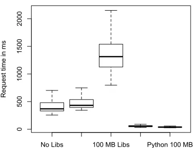
In Figure 3.1 we show the difference in loading request times between the Java and Python applications. The applications shown are:
• No Libs: in this Java application, all libraries were stripped from the war’s library directory
and the application was uploaded that way.
• Default Libs: in this application, the libraries in the application’s library directory were only
those placed there by default by the Google plugin for Eclipse.
• 100 MB Libs: in this application, 100 MB worth of jar files were added to the application’s
• Python: in this Python application, the only file uploaded was the .py file for the ’hello world’
application.
• Python 100 MB: in this Python application, 100 MB of additional .py files were added to the
application directory.
No Libs 100 MB Libs Python 100 MB
0 500 1000 1500 2000 R eq ue st ti me in ms
Figure 3.1: Differences in the loading request times for a ’hello world’ style application in Java and Python.
From the data we can see that the startup time of Python instances is substantially better than Java instances, even for very simple appli-cations. The median loading request response time of the simplest Java application was 369 milliseconds, while the median response time of the Python application was 54 milliseconds. For applications that are not particularly sensitive to latency, this initial difference is relatively in-substantial, however, the test with additional libraries added is more worrisome for Java users that rely on substantial frameworks. The me-dian response time for a loading request sent to the Java application with an artificially inflated library folder was 1,341 milliseconds.
These findings also corroborate findings from the operation of the Community Seismic Network. In Section 4.2.3 we will show that loading requests for our more sophisticated application, where libraries are actual dependencies, are even more troublesome.
It is worth noting here that the additional latency experienced for the 100 MB Libs application is roughly 1 second, which would correspond to about 1 Gbps when factoring in additional latency for finding and accessing the appropriate files. What this means is that most of the increased latency is likely attributable to being forced to download the entire application before the servlet could start. This is notable because it is clear from our tests that the equivalent Python application suffered no such delay. While the application package was still 100MB in size, the application was able to start before the entire application was downloaded. This is a substantial performance advantage for Python users.
requests should avoid large codebases, while language agnostic users needing to deal with loading requests may be best served by choosing Python. The final and most obvious takeaway from our data is that loading requests should be avoided where possible.
3.1.4.2 Avoiding loading requests
Loading requests occur for one of several reasons:
1. the application had no traffic at all for a period of time, did not use the Always On option, and was unloaded
2. the application experienced a small spike in traffic and did not use the Always On option
3. the application experienced a larger spike in traffic and it was faster to send requests directly to the new instances than to wait for new instances to warm up
The Always On feature permits users to pay for a fixed number of instances to always be on standby so that small surges in traffic are easily accommodated by the waiting instances without those incoming requests incurring the additional latency of a loading request. For applications with relatively smoothly varying load, this means that applications should be able to completely eliminate loading requests by paying for the feature. Applications which are more resilient to latency are unlikely to be bothered by the latency of loading requests, particularly since those requests are guaranteed to succeed (see results in Section 4.2.3).
Chapter 4
Case Study: Cloud Computing for
Earthquake Detection
4.1
The Problem
In the Earthquake Detection problem, the question being addressed is whether large groups of noisy sensors can create a good enough picture of a region to provide operationally useful shakemaps for damage assessment and whether or not these sensors, in concert, can arrive at a conclusion regarding the approximate location and strength of an earthquake faster than a traditional, sparse network operating with only very high quality sensors. This is similar to the work being explored by the Quake-Catcher Network[22], but my thesis is different in that it explores the use of public cloud computing platforms to support the application instead of Berkeley’s private BOINC system.
Since many sensors are needed to help address this problem, the bursty nature of the incoming traffic would pose obstacles for a simple client-server model or even for clustered server topologies. While traffic during quiescent periods is limited only to control traffic and false positives, traffic during seismic events could approach sensor density in a region. Initially, only those sensors closest to the source would send messages, but for a major seismic event the sustained nature of the event and the periodic resubmission of data implies that the requests per second rate would reach a significant fraction of the total number of sensors in the region. If we achieve a goal, for instance, of 10,000 sensors in a region like Southern California, we would expect most of the 10,000 sensors to send messages as the earthquake spreads outward, and to continue doing so for the duration of the earthquake.
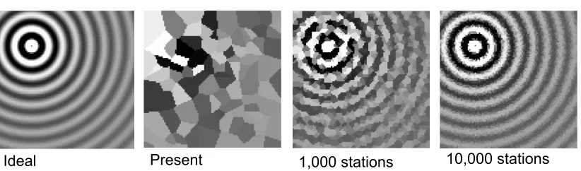
Present
Ideal
1,000 stations
10,000 stations
Figure 4.1: Increasing sensor density enables better visualization of earthquakes.
acquisition, deployment, and ongoing maintenance.
There are several advantages to a dense community network. First, higher densities make the extrapolation of what regions experienced the most severe shaking simpler and more accurate. In sparse networks, determining the magnitude of shaking at points other than where sensors lie is complicated by subsurface properties. As you can see in Figure 4.1, a dense network makes visualizing the propagation path of an earthquake and the resulting shaking simpler. With a dense network, we propose to rapidly generate a block-by-block shakemap that can be delivered to first responders within a minute.
Second, community sensors owned by individuals working in the same building can be used to establish whether or not buildings have undergone deformations during an earthquake which cannot be visually ascertained. This type of community structural modeling will make working or living in otherwise unmonitored buildings safer.
Lastly, one of the advantages of relying on cheap sensors is that networks can quickly be deployed to recently shaken regions for data collection or regions which have heretofore been unable to deploy seismic network because of cost considerations. As the infrastructure for the network lies entirely in the cloud, sensors deployed in any country can rely on the existing infrastructure for detection. No new infrastructure will need to be acquired and maintained, rather, one central platform can be used to monitor activity in multiple geographies.
4.2
The Architecture
region, and estimate the likelihood that an earthquake is occurring.
The use of Google App Engine, as opposed to a more traditional server format, is useful for several reasons. First, it means that the server itself cannot be rendered inaccessible by the natural event that it is attempting to detect. That is, in the case of a single physical server, a natural disaster could destroy the server or its connection to the outside world. In the best case, backups are available and limited data is lost, but in either case the server is not available for use at the time that it is most needed. Using the cloud model means that, while it is possible for some data in transit to be lost, the server and its data, being decentralized, will remain available during the time of crisis.
Second, the decentralized model means that deploying the application to multiple geographies is greatly simplified. Since the address used to talk to the Google App Engine application will actually redirect to the nearest available cluster, determining cluster placement for optimal access is handled automatically; thus, concerns over the need and method of deploying additional physical resources evaporate. Lastly, and perhaps most importantly, the solving of problems related to scale is no longer a direct concern of the project. Infrastructure placement, cluster sizing, distributed messaging, and more, are all problems that a team needs to deal with when building an application to scale. Using existing cloud solutions relies on previously developed solutions to the problems so that the actual focus of the project can be addressed.
Pick Registration Heartbeat
Datastore
Client Interaction Associator Early Warning Alerts
Google App Engine
Memcache
Figure 4.2: Overview of the CSN system. An overview of the CSN infrastructure is
presented in Figure 4.2. A cloud server admin-isters the network by performing registration of new sensors and processing periodic heart-beats from each sensor. Pick messages from the sensors are aggregated in the cloud to perform event detection. When an event is detected, alerts are issued to the community.
PaaS systems were investigated in general, and Google App Engine selected in particular, because of the ability to scale in small amounts of time from using minimal resources to
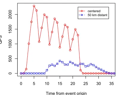
of the network and a maximum rate of 2,289 QPS for an earthquake centered relative to the sensor network.
4.2.1
Sensor messages
0 5 10 15 20 25 30 35
0
500
1000
1500
2000
Time from event origin
Q
PS
centered 50 km distant
Figure 4.3: Estimates of the amount of server traf-fic generated by a magnitude 5 earthquake at dif-ferent distances from the sensor network.
The CSN is designed to scale to an arbitrary number of community-owned sensors, yet still provide rapid detection of seismic events. It would not be practical to centrally process all the time series acceleration data gathered from the entire network, nor can we expect volunteers to dedicate a large fraction of their total band-width to reporting measurements. Instead, we adopt a model where each sensor is constrained to send fewer than a maximum number of sim-ple event messages per day to an App Engine fusion center.
Sensors in the network send three kinds of messages to the server.
Pick messages are sent when anomalous seismic activity is detected. They have very little payload, containing only the client’s identifier, the time of the event, the maximum amplitude experienced, and the location of the client at the time of detection. The process of pick detection is discussed in Section 4.4.
Heartbeat messages are sent once per hour to keep the server informed of which clients are
currently active. Clients can also relay waveforms of suspected events using the heartbeat messages.
Registration messages are sent by new clients to obtain a registration id, and by existing clients
to change registration values. The amount of traffic generated by these messages is small enough to be negligible.
4.2.2
Cost
To estimate the cost of running the CSN network at a larger sensor density, we must first estimate a general false positive rate, the amount of control data generated per sensor, and the amount of data from each sensor that we would like to store for analysis purposes.
average. Thus, we can conclude that our active clients generated 12.6 picks per day on average. Since the total number of picks includes those generated for testing or demo purposes, that is, intentionally generated picks, we can assume this is a safe upper bound on the false positive rate of our normal sensors. Per sensor studies that exclude intentionally generated picks will need to be conducted to more accurately narrow down the number of false picks expected to be generated per day.
Each pick requires 117 bytes to transmit. Each sensor, at network maturity, is expected to send 24 heartbeats per day. Each heartbeat requires 86 bytes to transmit. Using those figures to calculate the outbound and inbound bandwidth costs, it is clear that our main limiting factor is cpu. That is, it would take a network of 303,471 sensors at that size of message to use up the incoming bandwidth. If we letnbe the number of sensors in the network, we can then estimate the cpu cost of running the network as: c= (n(12.6(869(1−.218) + 5132·.218) + 24(3132(1−.282) + 7985·.282)) 1
3600000−6.5).1
Solving for 0 we get that a network of up to 179 sensors could be operated without generating a bill with additional sensors costing $0.00363 per sensor per day. These parameter estimates are conservative in several respects, however. First, they do not include the savings that could be generated by optimizations which reduce the amount of cpu consumed per request. Second, they do not include the costs associated with other overhead messages or the cost of data stored for archival purposes. The second point is more dependent on data retention policies, however. The first point is especially salient because of our discussion of loading times when comparing Python and Java.
The amount of cpu ms consumed per request could be easily driven down by switching to a language with a smaller loading request penalty. Additionally, these figures currently include the cpu penalty incurred by processing 1 MB waveforms with every heartbeat. In reality, the processing times of heartbeats should be lower than the processing times of picks; even setting them equal yields a network size of up to 323 sensors with nearly half the incremental cost per sensor. Finally, the cpu cost uses the loading request incidence rate from our network; in a larger network, we would expect the loading request rate to be much lower. Setting it to the overall loading request rate of the current network yields a network size of 541 sensors with an incremental cost of just $0.00120.
4.2.3
Performance
The biggest impact on system performance is the occurrence of loading requests, which were de-scribed in Section 3.1.4.
overall incidence rate of loading requests was only 7.34%. 0 2000 4000 6000 8000 R eq ue st ti me in ms Normal Heartbeat Loading Heartbeat Normal Pick Loading Pick
Figure 4.4: Latency for pick and heartbeat mes-sages for both normal and loading requests. Figure 4.4 shows that the penalty the CSN
application currently pays for a loading request is substantially higher than the minimal appli-cations explored in Section 3.1.4. That is, to process even a simple message, such as a pick, the median processing time increases from 202 ms to 3,246 ms, a difference of over 3 seconds. This is even greater than the worst penalty ex-perienced by our simple hello world applications and shows that, as one might expect, libraries that are in use can have a much more dramatic impact on instance startup time. Heartbeats paid a similar penalty, with the median process-ing time increasprocess-ing from 1,205 ms to 4,320 ms.
In the version of our application from which this information was derived, heartbeat and pick messages, despite structural dissimilarity, shared a common entry path in the application. It is therefore expected that the penalty paid by both messages would be similar.
4.2.3.1 Error rates
Error rates are another important factor. There are three types of errors we will include in our analysis of CSN error rates: deadline exceeded errors, aborted requests, and serious problems. Deadline errors were previously discussed as occurring when a request is terminated for exceeding the processing deadline imposed by App Engine. These errors are lumped together in the error rate, considered a fault of the PaaS provider, because the extreme variability in the processing of a request is not attributable to developer code, but rather to conditions within the cloud system.
All three types of errors that we measure have a 0% chance for loading requests. Take heartbeats again as an example. While the total error rate of non-loading requests was 1.33%, the error rate of loading request heartbeats was exactly 0%, giving an overall heartbeat error rate of 0.95%. This discrepancy in error rates leads us to believe that special priority is given to requests which hit a cold system, preventing them from encountering the same problems that normal requests might otherwise encounter.
4.2.3.2 Lessons learned
If the application is latency sensitive, use Python. The Java Virtual Machine was not designed
for scripting-style execution. That is, it was not set up to load, run a snippet of code, and then unload. It was designed to load once, with some known amount of overhead, and then process future bytecode efficiently. For security reasons, the App Engine team loads every Java application in its own JVM. Since loading requests must then wait on JVM initialization in addition to whatever costs are paid by the application, this is less than ideal. Conversely, Python has no such overhead; code that needs to be run, and just that code, can be swiftly retrieved and run. For programs that need to be insensitive to loading request penalties, Python is the clear winner for Google App Engine.
Develop direct no-dependency pathways for data retrieval and processing. In a standard server
installation, it is common to spend time setting up the environment before requests are ever handled. While this is possible on App Engine by utilizing the Always On feature, for any latency sensitive application that needs to endure loading requests, it is undesirable. Instead, building pathways into your code that allow time-sensitive data to arrive without loading dependencies from other parts of the application will ensure that you are able to drive down the instance startup time and the processing time of individual requests. The only way to effectively manage this in Java is with separate application versions or separate applications entirely (which might communicate by means of an API). In Python, dependencies which are not called by the code on the critical path will not affect the instance’s startup time; so as long as the particular logic lines leading to data processing do not invoke those dependencies, they can be buried elsewhere in the code.
4.3
Numeric Geocells for Geospatial Queries
resolution 14 geocell uses 14 bits, 7 for latitude and 7 for longitude, to encode the resolution. A resolution 25 geocell uses 25 bits, 12 for latitude and 13 for longitude.
It’s important to note that the ratio of the height to the width of a bounded area depends on the number of bits used to encode latitude and longitude. For even-numbered resolutions, an equivalent number of latitude and longitude bits are used. For odd numbered resolutions, one additional longitude bit is used. This permits bounding boxes with different aspect ratios. An odd numbered resolution at the equator creates a perfect square, while an even-numbered resolution creates a rectangle with a 2:1 ratio of height to width.
4.3.1
Creating geocells
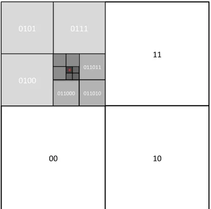
Geocells are created using a latitude, longitude pair. This is done by dividing the world into a grid and starting with the (90◦S, 180◦W), (90◦N, 180◦E) bounding box, which describes the entire world. Each additional bit halves the longitude or latitude coordinate space. Odd numbered bits, counting from left to right in a bit string, convey information about the longitude, while even-numbered bits convey information about the latitude. After selecting an aspect ratio by choosing even or odd numbered resolutions, geocells are made larger or smaller in increments of 2. This means that each larger or smaller geocell selected will have the same aspect ratio as the previous geocell.
11
10 00
0111 0101
0100
011011
011000 011010
Figure 4.5: How bounding boxes divide the coor-dinate space.
For this reason, each bit pair can be thought of as describing whether the initializing point lies in the northwest, northeast, southwest, or southeast quadrant of the current bounding box. Subsequent iterations use that quadrant as the new bounding box. To work a simple ex-ample, consider (34.14◦N, 118.12◦W). We first determine whether the desired point lies east or west of the mean longitude and then deter-mine whether it lies north or south of the mean latitude. If the point lies east of the mean lon-gitude, the longitude bit is set to 1, and if the point lies north of the mean latitude, the lati-tude bit is set to 1. In our example, the point lies in the northwest quadrant, yielding a bit pair of 01 for a resolution of 2. Iterating through the
algorithm yields the following bits for a resolution of 28:
For an illustration of how increasing resolution divides the coordinate space, see Figure 4.5. Because these representations are stored as fixed-size numbers, the resolution of the geocell must also be encoded. Otherwise, trailing zeros that are a result of a less than maximum resolution would be indistinguishable from trailing zeros that represent successive choices of southwest coordinates. Therefore, the last 6 bits of the long are used to encode the resolution. The other 58 bits are available for storing resolution information.
For space considerations, we also have an integer representation capable of storing resolutions from 1 to 27 using 4 bytes, as well as a URL-safe base64 string based implementation that uses a variable number of bytes to store resolutions from 1 to 58. The integer implementation uses 5 bits to store the resolution, and the remaining 27 bits are available for resolution information. The string based implementation always encodes the resolution in the final character, occupying 6 bits of information in 1 byte, while the remaining characters encode the resolution information.
Our analysis of geocell sizes at various resolutions led us to the conclusion that the most useful geocell sizes for event detection were resolutions 12 through 28. Resolution 29 ranges from 1.5 kilometers square to 0.65 kilometers square depending on the point on earth (see Limitations) and is too small to be useful for aggregation in all but the densest networks. Resolution 12 is quite large, encompassing anywhere from 84,000 square kilometers to 195,000 square kilometers. This resolution is still useful for aggregation of extremely rare events that may be spread out over a large region.
4.3.2
Comparison
Two similar open methods of hashing latitude and longitude pairs into simple strings have been previously proposed: GeoModel[23] and Geohash[24]. Our algorithm is capable of translating to and from representations in both systems. Numerous other systems exist; however, many are variations on a similar theme, and the earlier systems not designed for computer derivation each suffer from different shortcomings. The UTM[25] and MGRS[26] systems not only have a complicated derivation algorithm[27] but also suffer from exceptions to grid uniformity. The GARS[28] and GEOREF[29] system utilize an extremely small number of resolutions: 3 and 5, respectively. The NAC System[30] is proprietary and has different aims, such as being able to encode the altitude of a location.
serves at that hash.
Our numeric geocells have one key advantage over the Geohash and GeoModel algorithms: the numeric representation allows for the description of a broader range of resolutions. GeoModel and Geohash encode 4 and 5 bits of information per character, respectively, using the length of the character string to encode the resolution. Numeric geocells therefore have 4 to 5 times more expressive power in possible resolutions.
Resolution density has a strong impact on the number of cells required to cover a given region or the amount of extra area selected by the cells but not needed. When selecting cells to cover a region, it is possible that several smaller geocells could be compressed into one larger geocell. This can happen more often when more resolutions are available. For instance, 16 GeoModel cells and 32 Geohash cells compress into the next larger cell size, where only 4 numeric geocells compress into the next larger numeric geocell (when maintaining aspect ratio). This comes at the expense of having to store more resolutions in order to perform the compression. Section 4.3.4 contains more information on the selection of geocells to query.
Space filling curves, such as the Hilbert curve, can provide similar advantages by using an algo-rithm to ascribe addresses to all the vertices in the curve. Whatever advantage these curves might have derives from their visitation pattern, which can yield better aggregation results for queries that rely on ranges. Our query model utilizes set membership testing for determining geographic locality, which means that we cannot derive a benefit from the visitation pattern of space filling curves. We rely on the simpler hash determination method used in quad trees instead.
4.3.3
Limitations
Because they rely on the latitude and longitude coordinate space, numeric geocells and similar algo-rithms all suffer from the problem that the bounded areas possess very different geometric properties depending on their location on Earth. The only matter of vital importance is the coordinate’s lat-itude; points closer to the equator will have larger, more rectangular geocells while points farther from the equator will have smaller, more trapezoidal geocells.
Jakarta Caltech London Reykjavik
A:Jakarta 1 0.83 0.63 0.44
H:W Even 1.99 1.66 1.24 0.87
H:W Odd 0.99 0.83 0.62 0.44
Finally, prefix matching with any of these algorithms suffer from poor boundary conditions. While geocells which share a common prefix are near each other, geocells which are near each other need not share a common prefix. In the worst case scenario, two adjacent geocells that are divided by either the equator, the Prime Meridian or the 180th Meridian will have no common prefix at all. For this reason, geocells are used exclusively for equality matching.
4.3.4
Queries
When querying for information from the Datastore or Memcache, geocells can be used to identify values or entities that lie within a given geographic area. A function of the numeric geocell library allows for the southwest and northeast coordinates of a given area, such as the viewable area of a map, to be given and returns a set of geocells which covers the provided area. Given that no combination of geocells is likely to exactly cover the map area, selecting a geocell set to cover a specified area is a compromise between the number of geocells returned and the amount of extraneous area covered.
Figure 4.6: Combining geocells of multiple resolu-tions to cover an area.
With smaller geocells, less area that is not needed will be included in the returned geocells, however, more geocells will be required to cover the same geographical area. Larger geocells will require a smaller number of geocells in the set, but are more likely to include larger swaths of land that lie outside the target region. Balanc-ing these two factors requires a careful choice of cost function which takes into account the cost of an individual query for a specific size, which depends on the network density.
With a low density, smaller numbers of queries across larger parcels of land are opti-mal as discarding the extraneous results is less costly than running larger numbers of queries. With very high sensor densities, too many
Another feature of numeric geocells is that smaller cells can be easily combined to form larger cells. If an object stores the geocells that it exists within at multiple resolutions, then any of those resolutions can be used for determining whether or not it lies within a target geographical area. The algorithm for determining the set of geocells to query can then combine several smaller geocells into larger geocells, which allows larger geocells to be used in the interior of the map with smaller geocells along the exterior.
For instance, Figure 4.6 shows how smaller geocells can be combined into larger geocells of varying sizes. Importantly for our purposes, the determination of neighboring geocells is a simple and efficient algorithm. By using minor bit manipulations, it is possible to take a known geocell and return the geocell adjacent to it in any of the four cardinal directions. This means that if an event arrives at a known location, not only can the cell that the event belongs to be easily identified but the neighboring cells. This factors in to our event detection methods, which are described next.
4.4
Decentralized Detection with Community Sensors
The CSN system performs decentralized detection of seismic events by allowing each individual sensor to generate picks of potential seismic events and then aggregating these pick messages by geocell in the cloud to determine if and where an event has occurred. The different algorithms used at the sensor and server levels are discussed next.
4.4.1
Sensor-side Picking Algorithms
Different sensor types are likely to experience different environmental and noise conditions, and so different picking algorithms may be best suited to particular sensor types. We studied two picking algorithms: the STA/LTA algorithm, designed for higher-quality sensors in relatively low-noise environments, and a density-based anomaly detection algorithm suited to handling the complex acceleration patterns experienced by a cell phone during normal daily use. These algorithms are described in detail in [31] and summarized here.
Event Detection using Averages: STA/LTA STA/LTA (Short Term Average over Long Term
the STA/LTA.
4.4.2
Server-side Pick Aggregation
Picks generated by the sensors are sent to the App Engine server. These simple events are aggregated using the numeric geocells described in Section 4.3. However, a few factors complicate complex event association and detection.
First, the time of App Engine instances is not guaranteed to be synchronized with any degree of accuracy. This means that relative time determination within the network must be handled by clients if any guarantees about clock accuracy are to be made. This is currently done through the inclusion of an NTP client in the sensor software which determines the drift of the host computer to the network time at hourly intervals.
Second, requests may fail for a variety of reasons. We have previously estimated that as many as 1% of requests on App Engine will fail for reasons beyond the control of the developer. These kinds of errors include requests that wait too long to be served, hard deadline errors, and serious errors with the App Engine servers. In addition to these system errors, clients may go offline without notice due to a software error or something as simple as the host computer going to sleep.
These system conditions mean that the detection algorithm must be: insensitive to the reordering of arriving messages, which occurs by variations in processing or queueing time or by inconsistent determination of network time, and insensitive to the loss of small numbers of messages either due to client or server failures.
The server’s job is to estimate complex events such as the occurrence of an earthquake from simple events that indicate an individual sensor has experienced seismic activity. This is done by estimating the frequency of arriving picks by allocating arriving picks to buckets. Buckets are created by rounding the pick arrival time to the nearest two seconds and appending the geocell to the long representation of the time. This gives a unique key with which a bucket is created that all arriving picks in the same time window and region will use to create estimates of the number of firing sensors at that point in time. For instance, an example bucket name would be ‘12e55d89260-4da040500000001c’.
active clients to determine whether or not a specific geocell has exceeded a threshold level of activity to perform further computation. This is the first trigger which generates a complex event that a given geocell has activated. Activation of the geocell is managed by a Task Queue job which is created to proceed with further analysis. The job is named, which means that for any number of arriving picks in the same time window, only one job will be created per geocell per time window.
Chapter 5
Case Study: Cloud Computing for
Unstructured Text Analysis
Our experiments with unstructured text analysis explore how the composition of multiple SaaS web components can lead to useful results. Specifically, our text analysis platform makes use of a single server for staging requests to a SaaS application which provides the content of all posts in the blogosphere and pushes those requests to a second SaaS application which rerenders the unstructured text as an RDF document composed of its referenced entities. The data flow for this application can be see in Figure 5.1.
! "
acquisition of Spinn3r data
submission of post to Calais for processing # $ processing of RDF annotated data % time series analysis of extracted entities and relationships
enrichment of events with IEM
market data & PIB selects device to deliver
notification to
device receives, interprets, and delivers event
'
Figure 5.1: caption
The Personal Information Broker A
per-sonal information broker (PIB) acquires and analyzes data from multiple sources, detects events, and sends event objects to appropriate devices such as cell phones, PDAs and comput-ers. A PIB also displays data in multiple dash-boards. A PIB may acquire data from blogs, news stories, social networks such as Facebook,
Twitter, stock prices and electronic markets. In this paper we restrict attention to PIBs that analyze blogs.
Spitzer — the input to the application is only the entity, i.e., Clinton, of interest. Related entities are discovered by monitoring other entities that co-occur with the entity of interest and estimating the relevance of the co-occurance at each point in time that it is found in the stream. The changing numbers of posts containing the monitored entity and the related entity is detected automatically by the application. The challenge is to carry out this detection in near real-time as opposed topost
facto data mining.
!" #!!" $!!" %!!" &!!" '!!" (!!" )!!"
$*#)" $*#+" $*$#" $*$%" $*$'" $*$)" $*$+" %*$" %*&" %*(" %*," %*#!" %*#$" %*#&" %*#(" %*#,"
Figure 5.2: Volume of posts mentioning both ”Clinton” and ”Spitzer” over time.
Information in the blog universe can be cor-related automatically with other types of data such as electronic markets. For instance, when a component of a PIB detects anomalous time series patterns of blog posts associating a pres-idential candiate, say Senator Obama, with some other entity, say Rev. Jeremiah Wright, then it can determine whether Senator Obama’s “stock” price on the Iowa Electronic Market changed significantly at that time. If the price of Senator Obama’s stock didn’t change much
then we may deduce (though the deduction may be false with — we hope — low probability) that market makers don’t expect this association to have much impact on the likelihood of Senator Obama’s chances of winning.
Another PIB application continuously searches for entities to discover when the rate of blog posts containing names ofany of these entities changes rapidly. This application has no input — it detects changes in the frequency of posts about any and all entities. For example, the application can discover that the volume of posts about the bank IndyMac changed significantly on July 8 and July 12 (see Figure 5.3). The event that is detected does not predict anything; the event is merely an anomaly in the time-series patterns of posts about any entity. In this example, the failure of IndyMac became public knowledge on July 11.
5.1
Experimental Results
!" #!!" $!!" %!!" &!!" '!!" (!!"
()$$)$ !!*" ()$&)$ !!*" ()$()$ !!*" ()$*)$ !!*" ()%!)$ !!*" +)$)$! !*" +)&)$! !*" +)()$! !*" +)*)$! !*" +)#!)$ !!*" +)#$)$ !!*" +)#&)$ !!*" +)#()$ !!*" +)#*)$ !!*" +)$!)$ !!*" +)$$)$ !!*" +)$&)$ !!*"
Figure 5.3: Volume of posts about IndyMac over time.
The first three steps of the application de-scribed by the information flow in Figure 5.1 were implemented; a database is used to store processed data for later processing to analyze missed event opportunities and run simulations of input streams. Using this data, algorithms for detecting events in the stream are being de-veloped to help complete the implementation of step 4.
The stream itself is relatively large; over 14 weeks of data, the database has increased to 164GB, or about 1.7GB per day. The average
number of posts for a given weekday is 292,879, but, being bursty in nature, the number of posts in a timeframe varies dramatically, from 0 messages in a given second to upwards of 30. Weekends see only 76% of the traffic that weekdays see, or an average of 223,124 posts. Algorithms that smooth frequencies over time need to account for the discrepancies in post volumes between weekdays and weekends or holidays; without accounting for this discrepancy, erroneous events can be generated by an algorithm which incorporates that discrepancy as part of its algorithm for detecting significant changes.
It is worth noting that, out of a sample of 31,304,036 processed posts, only 21,741,604 posts actually entered the database. The singular criterion for entering the database is that Calais has identified at least one entity that the post referred to. This indicates that only roughly 70% of the processed posts contain any meaningful content that can be analyzed for generating events. The ability to identify and discard the 30% of posts that are meaningless before they are processed would yield large performance gains, both locally for the corresponding process and remotely for the Calais web service.
posts, which includes errors from posts that are too large to process and non-English posts that slipped through Spinn3r’s language filter.
Chapter 6
Conclusion
Bibliography
[1] (2011, 4) Project budburst. [Online]. Available: http://www.windows.ucar.edu/citizen science/ budburst/
[2] (2011, 4) Carson. [Online]. Available: http://www.marylandsciencecenter.org/exhibits/Carson. html
[3] (2011, 4) Christmas bird count. [Online]. Available: http://www.audubon.org/bird/cbc
[4] (2011, 4) Netflix prize. [Online]. Available: http://www.netflixprize.com/
[5] (2011, 4) Wikipedia. [Online]. Available: http://www.wikipedia.org/
[6] B. P. Rimal, E. Choi, and I. Lumb, “A taxonomy and survey of cloud computing systems,”
International Joint Conference on INC, IMS and IDC, Jan 2009.
[7] (2011, 2) Amazon ec2. [Online]. Available: http://aws.amazon.com/ec2/
[8] (2011, 2) Rackspace cloud servers. [Online]. Available: http://www.rackspacecloud.com/ cloud hosting products/servers
[9] (2011, 2) Amazon ec2 faqs. [Online]. Available: http://aws.amazon.com/ec2/faqs/
[10] (2011, 3) Google app engine. [Online]. Available: http://code.google.com/appengine/
[11] (2011, 3) Gmail. [Online]. Available: http://mail.google.com/
[12] (2011, 3) Photoshop online. [Online]. Available: http://www.photoshop.com/tools?wf=editor
[13] (2011, 3) Zoho office suite. [Online]. Available: http://www.zoho.com/
[14] Y. Jie and Q. Jie. . . , “A profile-based approach to just-in-time scalability for cloud applica-tions,”Cloud Computing, Jan 2009.
[15] L. Vaquero and L. Rodero-Merino. . . , “Dynamically scaling applications in the cloud,” ACM
[16] S. Schneidert, H. Andrade, B. Gedik, K.-L. Wu, and D. S. Nikolopoulos, “Evaluation of stream-ing aggregation on parallel hardware architectures,” inProceedings of the Fourth ACM
Interna-tional Conference on Distributed Event-Based Systems, ser. DEBS ’10. New York, NY, USA:
ACM, 2010, pp. 248–257.
[17] (2011, 2) Google app engine downtime notify. [Online]. Available: http://groups.google.com/ group/google-appengine-downtime-notify
[18] (2011, 3) High-replication datastore. [Online]. Available: http://code.google.com/appengine/ docs/python/datastore/hr/
[19] (2011, 3) Heroku. [Online]. Available: http://www.heroku.com/
[20] (2011, 3) Amazon web services elastic beanstalk. [Online]. Available: http://aws.amazon.com/ elasticbeanstalk/
[21] (2011, 2) The webapp framework. [Online]. Available: http://code.google.com/appengine/ docs/python/tools/webapp/
[22] E. Cochran and J. Lawrence, “The quake-catcher network: Citizen science expanding seismic horizons,” Seismological Research Letters, vol. 80, p. 26, Jan 2009. [Online]. Available:
http://srl.geoscienceworld.org/cgi/content/extract/80/1/26
[23] S. S. Roman Nurik. (2011, 3) Geospatial queries with google app engine using geomodel. [Online]. Available: http://code.google.com/apis/maps/articles/geospatial.html
[24] geohash.org. (2011, 3) Geohash. [Online]. Available: http://en.wikipedia.org/wiki/Geohash
[25] DMATM 8358.2 The Universal Grids: Universal Transverse Mercator (UTM) and Universal
Polar Stereographic (UPS), Defense Mapping Agency, Fairfax, VA, 9 1989.
[26] DMATM 8358.1 Datums, Ellipsoids, Grids, and Grid Reference Systems, Defense Mapping
Agency, Fairfax, VA, 9 1990.
[27] Locating a position using utm coordinates. [Online]. Available: http://en.wikipedia.org/wiki/ Universal Transverse Mercator
[28] L. Nault, “Nga introduces global area reference system,”PathFinder, 11 2006.
[29] (2011, 3) Georef. [Online]. Available: http://en.wikipedia.org/wiki/Georef
[31] M. Faulkner, M. Olson, R. Chandy, J. Krause, K. M. Chandy, and A. Krause, “The Next Big One: Detecting Earthquakes and Other Rare Events from Community-based Sensors,”
inProceedings of the 10th ACM/IEEE International Conference on Information Processing in