Volume 2009, Article ID 475147,7pages doi:10.1155/2009/475147
Research Article
Finite Sample FPE and AIC Criteria for Autoregressive Model
Order Selection Using Same-Realization Predictions
Shapoor Khorshidi and Mahmood Karimi
Department of Electrical Engineering, Shiraz University, Shiraz 71348-51151, Iran
Correspondence should be addressed to Mahmood Karimi,[email protected]
Received 26 May 2009; Revised 2 November 2009; Accepted 31 December 2009
Recommended by Abdelak Zoubir
A new theoretical approximation for expectation of the prediction error is derived using the same-realization predictions. This approximation is derived for the case that the Least-Squares-Forward (LSF) method (the covariance method) is used for estimating the parameters of the autoregressive (AR) model. This result is used for obtaining modified versions of the AR order selection criteria FPE and AIC in the finite sample case. The performance of these modified criteria is compared with other same-realization AR order selection criteria using simulated data. The results of this comparison show that the proposed criteria have better performance.
Copyright © 2009 S. Khorshidi and M. Karimi. This is an open access article distributed under the Creative Commons Attribution License, which permits unrestricted use, distribution, and reproduction in any medium, provided the original work is properly cited.
1. Introduction
Let a real AR process be given by
x(n)=a1x(n−1) +· · ·+apx
n−p+ε(n), (1)
where p is the order of the process, a1,. . .,ap are the
real coefficients of the process, and ε(n) is an independent and identically distributed (i.i.d.) random process with zero mean and varianceσ2
ε. The processε(n) is the input process
to the AR model. It is assumed that x(·) is mean and covariance ergodic; so the poles of the AR model are inside the unit circle.
Suppose thatx(1),. . .,x(N) are consecutive samples of a sample function of the AR process x(·) given by (1). In addition, suppose that an arbitrary nonnegative integerqis considered as the true process order. The usual estimator for a nonrandom set of parameters is the maximum likelihood estimator (MLE) [1]. However, the exact solution of the MLE for the parameters of an AR(q) process is difficult to obtain [1]. IfN q, each of the AR estimation methods Least-Squares-Forward (LSF), Least-Least-Squares-Forward-Backward (LSFB), and Burg and Yule-Walker [1–3] is an approximation
of the MLE. In this paper, we use the LSF method to estimate a model as
x(n)=a1x(n−1) +· · ·+aqx
n−q+ε(n), (2) where ai’s are the LSF estimates of the AR parameters.
Residual variance, denoted by S2(q), is a measure of the
fitness of the above model to the data that have been used for estimating the parameters. It is defined as
S2q= 1 N−q
N
n=q+1 ⎡
⎣x(n)−q
i=1
aix(n−i)
⎤ ⎦ 2
. (3)
In the literature, two different kinds of predictions under model (1) are considered. For independent-realization pre-dictions, the aim is to predict the future of another indepen-dent series which has exactly the same probabilistic structure as the observed one. One special feature of this type of prediction is that its mathematical analysis is relatively easy. The independent-realization prediction error is defined as follows:
PEq=Ey
⎧ ⎪ ⎨ ⎪ ⎩ ⎡
⎣y(n)−q
i=1
aiy(n−i)
⎤ ⎦ 2
|x(1),. . .,x(N) ⎫ ⎪ ⎬ ⎪ ⎭,
where y(·) is another independent series which has exactly the same probabilistic structure as x(·), and Ey{·} is the
expectation operator over this independent series. However, for the practitioner, the emphasis is usually placed on same-realization predictions, that is, on the prediction ofx(N+h),
h≥1 givenx(1),. . .,x(N). The same-realization prediction error is defined as follows:
PEq
=E
⎧ ⎪ ⎨ ⎪ ⎩ ⎡
⎣x(N+h)−q
i=1
aix(N+h−i)
⎤ ⎦ 2
|x(1),. . .,x(N) ⎫ ⎪ ⎬ ⎪ ⎭.
(5)
In (4) and (5), ai’s are the LSF estimates of ai’s using
x(1),. . .,x(N). Note that in the expectation in (4) y(n) is independent of the ai’s, but in the expectation in (5),
x(N + h) depends on the ai’s. This difference causes the
prediction errors in (4) and (5) to be different. Almost all existing AR order selection criteria have been derived for independent-realization data. The independency is not a natural property for time series data, because when new observations of a time series become available, they are usually dependent on the previous data. So far, few time series model selection theories have been established without this unnatural assumption. In addition, the use of most of these model order selection criteria has not been justified for the same-realization case. Akaike information criterion (AIC) [4], final prediction error (FPE) criterion [5], Bayes information criterion (BIC) [6], minimum description length (MDL) criterion [7], Kullback information criterion (KIC) [8], corrected AIC (AICC) [9], and corrected KIC
(KICC) [10] are examples of the criteria that have been
derived for the large sample and independent-realization case. In [11, 12], Ing and Wei justified the use of FPE and AIC as AR order selection criteria in the large sample and same-realization case. Ing and Wei [11] presented a theoretical verification that AIC and FPE are asymptotically efficient (in the sense of the mean square prediction error) for same-realization predictions. When the underlying AR model is known to be stationary and of infinite order, Ing and Wei [11] showed that the values of the expectations of the squared prediction error for independent- and same-realization cases, with the order selected by FPE or AIC, have the same asymptotic expressions. Recently, Ing [12] removed the infinite-order assumption and verified the asymptotic efficiency of several information criteria, including FPE and AIC, for both finite- and infinite-order stationary AR models.
The order selection criteria obtained in the large sample and independent-realization case are not dependent on the method of estimation of the AR parameters. In other words, these criteria are identical for all AR parameter estimation methods. However, it is well known that, in the finite sample and independent-realization case, the performance of the order selection criteria depends on the parameter estimation method and it is necessary to derive different order selection criteria for each parameter estimation method [13–18].
In this paper, we derive a new estimate of the same-realization prediction error in the finite sample case and for the LSF parameter estimation method. We will use this new estimate to derive same-realization versions of FPE (FPEF) and AIC (AICF) in the finite sample case.
The remainder of this paper is organized as follows. In
Section 2, a new theoretical approximation is derived for the expectation of same-realization prediction error in the case that the LSF method is used. Based on this approximation, the FPEF criterion is introduced. In Section 3, the AICF criterion is introduced. In Section 4, simulated data are used for comparing the performance of the proposed order selection criteria with that of the existing criteria. In
Section 5, the conclusions of this paper are discussed.
2. Estimation of the Same-Realization
Prediction Error
Suppose that we have N observation data of the AR model defined by (1) asx(1),x(2),. . .,x(N). We define the following vectors and matrices for the case that the candidate orderqis greater than or equal to the true order (q≥p), and
Tstands for a transposed operation:
βA=
a1,a2,. . .,ap, 0,. . ., 0
T
q×1, (6) xi=
x(i),x(i+ 1),. . .,xN−q+i−1T, (7)
x(i)=x(i),x(i−1),. . .,xi−q+ 1T, (8)
XA=
xq xq−1 · · · x1
, (9)
εq+1=
εq+ 1,. . .,ε(N)T, (10)
x=[x(1),. . .,x(N)]. (11)
It follows from (1), (6), (7), (9), and (10) that
xq+1=XAβA+εq+1; q≥p. (12)
We use the LSF method to obtain the least-squares estimate ofβAas follows:
bA=
a1,a2,. . .,aq
T
=XTAXA
−1
XTAxq+1. (13)
The one-step same-realization prediction error is given by
PEq=Ex(N+ 1)−xq(N+ 1)
2
|x
, (14)
where xq(N + 1) is the linear predictor of x(N+ 1) given
x(1),. . .,x(N), that is,
xq(N+ 1)= q
i=1
aix(N+ 1−i)=xT(N)bA. (15)
It follows from (1), (6), and (8) that
Substituting (15) and (16) into (14), we can rewrite (14) as
PEq=ExT(N)βA+ε(N+ 1)−xT(N)bA
2
|x
. (17)
Using (12) and (13),xT(N)b
Acan be written as
xT(N)bA=xT(N)
XTAXA
−1 XTAxq+1
=xT(N)XT AXA
−1 XT
AXAβA
+xT(N)XTAXA
−1 XTAεq+1
=xT(N)βA+xT(N)XTAXA
−1
XTAεq+1; q≥p.
(18)
Combining (17) and (18), we have
PEq=E
ε(N+ 1)−xT(N)XT AXA
−1 XTAεq
+1 2
|x
=Eε(N+ 1)2|x
+E
xT(N)XT AXA
−1 XTAεq
+1 2
|x
−2E
ε(N+ 1)xT(N)XTAXA
−1
XAεqT +1|x
;
q≥p.
(19)
The value of the first term in the right-hand side of (19) is given as
Eε(N+ 1)2|x=Eε(N+ 1)2=σ2
ε. (20)
In (19), we know that ε(N + 1) is independent of the past samples of x(1),x(2),. . .,x(N), and ε(1),ε(2),
. . .,ε(N) for the AR process. In addition, the expres-sionxT(N)(XT
AXA)−1XTAεq+1 is a combination of x(1),x(2), . . .,x(N),ε(1),ε(2),. . .,ε(N). So,ε(N+ 1) is independent of
xT(N)(XT
AXA)−1XTAεq+1, and the third term of the right-hand
side of (19) is equal to zero:
E
ε(N+ 1)xT(N)XT AXA
−1 XAεqT
+1|x
=0. (21)
It follows from (12) that the value of the second term of the right-hand side of (19) is equal to
xT(N)XT AXA
−1 XTAεq
+1
=xT(N)XTAXA
−1 XAT
xq+1−XAβA
; q≥p.
(22)
The expressionxT(N)(XT
AXA)−1XAT(xq+1−XAβA) is a
com-bination ofx(1),x(2),. . .,x(N). So, it follows from (22) that
the expectation ofxT(N)(XT
AXA)−1XTAεq+1givenxis equal to xT(N)(XT
AXA)−1XTAεq+1, that is, E
xT(N)XT AXA
−1 XAεqT
+1 2 |x =
xT(N)XTAXA
−1 XTAεq+1
2
; q≥p.
(23)
Therefore, using (20), (21), and (23), we can rewrite (19) as
PEq=σ2
ε +
xT(N)XT AXA
−1 XTAεq+1
2
. (24)
Taking the expectation of PE(q) over the vectorx, it follows from (24) that
Ex
PEq=σ2
ε +Ex
xT(N)XT AXA
−1 XTAεq
+1 2
. (25)
It can be seen from (7)–(10) that
XTAεq+1=
xq xq−1 · · · x1 T
εq+1
=xq xq+ 1 · · · x(N−1)εq+1
=
N−1
i=q
x(i)ε(i+ 1).
(26)
Substituting (26) into (25), we obtain
Ex
PEq=σ2
ε+Ex ⎧ ⎪ ⎨ ⎪ ⎩ ⎡
⎣xT(N)XT AXA
−1N−1
i=q
x(i)ε(i+1) ⎤ ⎦
2⎫⎪⎬
⎪ ⎭. (27)
It is assumed that x(·) is a zero mean and covariance ergodic process. So, we define the covariance matrixR and its estimateRin the following way:
R=Ex(i)xT(i), (28)
R=
XT AXA
N−q. (29)
Using (29) and (27), we have
Ex
PEq
=σ2
ε +
1
N−q2Ex
⎧ ⎪ ⎨ ⎪ ⎩ ⎡
⎣xT(N)R−1
N−1
i=q
x(i)ε(i+ 1) ⎤ ⎦
2⎫⎪⎬
⎪ ⎭. (30)
To obtain a value for (30), we make the assumption that for sufficiently large (N−q):|RR −1−I
q|<1, where|A|is the
Euclidean norm of matrixA. Under this assumption, it is shown in [19] that
1
N−q2Ex
⎧ ⎪ ⎨ ⎪ ⎩ ⎡
⎣xT(N)R−1
N−1
i=q
x(i)ε(i+ 1) ⎤ ⎦
2⎫⎪⎬
⎪ ⎭
= q
N−qσ 2
ε +O
1
N−q3/2 ; q≥p,
whereβn=O(αn) means that for some positive numberM,
|βn| ≤M|αn|for everyn.
Substituting (31) into (30), we get
Ex
PEq=σ2
ε +
q
N−qσ 2
ε +O
1
N−q3/2 ; q≥p.
(32)
WhenN−qtends to infinity, the third term in the right-hand side of (32) tends towards zero faster than the other terms. So, for large enough values ofN−q
Ex
PEq≈
1 + q
N−q σ 2
ε; q≥p. (33)
It is shown in [16,17] that
Ex
S2q≈
1− q
N−q σ 2
ε; q≥p. (34)
Combining (33) and (34), we obtain
EPEq≈
1 +q/N−q
1−q/N−q E
S2q; q≥p. (35)
The above relation can be used for estimating PE(q) in the following way:
PEq=
1 +q/N−q
1−q/N−q S
2q; q≥p. (36)
It is reasonable to choose the integerq that minimizes this estimate of prediction error as the appropriate order for the AR process. So, we propose the finite sample FPE (FPEF) criterion as
FPEFq=
1 +q/N−q
1−q/N−q S
2q. (37)
The FPE criterion, which is an asymptotic estimate of the independent-realization prediction error, is defined in the following way [5]:
FPEq= N+q
N−qS
2q=
1 +q/N
1−q/N S
2q. (38)
As we mentioned earlier, the criterion defined by (38) is also used in the independent-realization case. WhenN q, the FPE criterion given by (38) is an approximation of FPEF. In the asymptotic caseN → ∞the criteria FPE and FPEF become identical.
3. AICF Criterion
We now give a mathematical derivation for finite sample AIC (AICF) criterion in the same-realization case starting from Kullback-Leibler (K-L) information. The K-L information is a measure of the distance between the true and the approximating pdfs for the data generated by the true pdf.
The K-L information for the approximating modelg(x|θ) is given by [20]
If,g(· |θ)=
!
f(x) ln
f(x)
g(x|θ) dx, (39) wherexis a vector of data generated by the true pdf f. We look for a uniqe value of parameter vectorθ, denoted byθ0,
that minimizes the K-L information. So,θ0is the solution to
the following optimization problem [20]:
min θ∈Θ "
If,g(· |θ)#=
!
f(x) ln
f(x)
g(x|θ0) dx, (40) whereΘis the parameter space. In fact, we have to find the model order and the parameter values that minimize (39).
The expression in the right-hand side of (39) is not dependent on the observed data and f is unknown. So, we cannot compute (39) for different values ofθand determine the valueθ0that minimizes the K-L information. Therefore,
we rewrite the K-L information in the following way:
If,g(· |θ)
=
!
f(x) lnf(x)dx−
!
f(x) lng(x|θ)dx
=constant−Exlng(x|θ).
(41)
The first term in the right-hand side of (41) is not dependent onθ. So, instead of minimizing (41), we can minimize the following term:
−Exlng(x|θ). (42) Note that the expression (42) is not dependent onx, but it depends onθ. The parameter vectorθ is unknown. So, in order to obtain an estimate of (42) we can replace θby its estimate. Suppose that N observations x(1),x(2),. . .,x(N) are available. Thus, for each model order, it is reasonable to replace θ by its maximum likelihood estimate θ which is a function of the observed data. As θ is the maximum likelihood estimate ofθ, this replacement minimizes (42) for each value of the model order. Now, in a slightly simplified notation, minimizing the K-L information changes to mini-mizing the Kullback-Leibler index given by
Δ=Ex
−2 lngx|θ(x),x, (43)
where θ is the maximum likelihood estimator of θ given the observed data vectorx, andg[x | θ] is the likelihood function. Usually, instead of using the exact maximum likelihood estimator ofθ, an approximation of it is used as
θin (43).
estimator of the AR parameter vectorθ),x(the future data of the AR model that depends on the observed data), andx
(vector of the observed data of the AR model) are defined as follows:
θ=bT A,σε2
T
, (44)
x=x(N+ 1), (45)
x=[x(1),x(2),. . .,x(N)]=x. (46)
Substituting (44)–(46) into likelihood functiong(x|θ,x), we obtain
gx|θ,x=gx(N+ 1)|bA,σε2,x
. (47)
When the input process ε(n) to the AR model is white Gaussian noise (WGN),g[x(N+1)|bA,σε2,x] can be written
as
gx(N+1)|bA,σε2,x
=exp
−x(N+1)−xT(N)b A
2 /2σ2
ε
√
2πσε .
(48)
Taking logarithm from both sides of (48), we get
lngx|θ,x=lngx(N+ 1)|bA,σε2,x
= −ln√2π−ln(σε)
−
x(N+ 1)−xT(N)b A
2
2σ2
ε
.
(49)
Substituting (45) and (49) into (43), we have
Δ= −Ex(N+1) "
2 lngx(N+ 1)|bA,σε2,x
#
=2Ex(N+1)
ln√2π+ ln(σε)
+
x(N+ 1)−xT(N)b A
2
2σ2
ε
|bA,σε2,x
=2 ln√2π+ 2 ln(σε).
+Ex(N+1)
x(N+ 1)−xT(N)b A
2
|bA,x
σ2
ε
.
(50)
The parameter σ2
ε in (50) can be replaced by the residual
varianceS2(q) given by (3). Thus, combining (14), (15), and
(50), we obtain
Δ=ln(2π) + lnS2q+PE
q
S2q. (51)
The prediction error PE(q) is unknown; so we replace it by its estimate given by (36) to obtain
Δ≈ln(2π) + lnS2q+
1 +q/N−q
1−q/N−q ; q≥p. (52)
The orderqthat minimizes (52) can be selected as the best AR model order. So, omitting the constant ln(2π) from (52), we obtain the finite sample AIC (AICF) criterion for AR model order selection in the same-realization case as
AICFq=lnS2q+
1 +q/N−q
1−q/N−q . (53)
The AIC criterion, which was derived for the independent-realization case, is defined in the following way [4]:
AICq=lnS2q+2q
N. (54)
4. Simulation Results
To investigate the effectiveness of the proposed criteria FPEF and AICF, we consider the problem of autoregressive model order selection for simulated data. The simulated data have been produced by AR(0), AR(1), AR(2), AR(3), and AR(7) processes defined as follows:
x[n]=ε(n),
x[n]=.95x[n−1] +ε(n),
x[n]= −1.4x[n−1]−.5x[n−2] +ε(n),
x[n]=−1.08x[n−1]−0.37x[n−2]−0.042x[n−3]+ε(n),
x[n]=2.8x[n−1]−3.22x[n−2] + 1.96x[n−3]
−.68x[n−4] +.13x[n−5]−.013x[n−6]
+.0005x[n−7] +ε(n),
(55)
whereε(n) is WGN with zero mean and varianceσ2
ε =1. We
can define the SNR parameter for each AR model as the ratio of the average output power of the AR model toσ2
ε in dB. The
SNRs of AR(0), AR(1), AR(2), AR(3), and AR(7) models are 0 dB, 10 dB, 10.13 dB, 5.11 dB, and 23 dB, respectively.
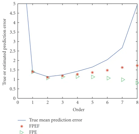
For each of the four models given by (55), 5000 inde-pendent simulation runs of 20 consecutive samples of the AR process were generated. In each simulation run, the first nineteen samples were used for estimating the coefficients of the AR model, and the last sample was used for computing the prediction error. Candidate orders were considered from 0 to 8. For each candidate order, the prediction error has been approximated by averaging over 5000 simulation runs. This true prediction error and the estimated prediction errors given by FPE and FPEF are shown for AR(0), AR(1), AR(2), AR(3), and AR(7) models in Figures 1, 2, 3, 4, and 5, respectively. These figures illustrate that when q/N is not small, the FPEF gives an estimate of the prediction error that is much better than FPE.
0 1 2 3 4 5 6 7 8 0.5
1 1.5 2 2.5 3 3.5 4
Order
T
rue
o
r
estimat
ed
p
re
dictio
n
er
ro
r
True mean prediction error FPEF
FPE
Figure 1: Estimation of prediction error for simulated AR(0) sequence withN=19.
0 1 2 3 4 5 6 7 8
0 0.5 1 1.5 2 2.5 3 3.5 4 4.5 5
Order
T
rue
o
r
estimat
ed
p
re
dictio
n
er
ro
r
True mean prediction error FPEF
FPE
Figure 2: Estimation of prediction error for simulated AR(1) sequence withN=19.
Table 1: Mean of prediction error for several order selection criteria.
Criterion
MPE FPE FPEF AIC AICF
order
AR(0) .31 3.35 2.02 3.17 1.02 AR(1) .48 3.92 2.78 3.99 1.32 AR(2) .51 4.42 2.87 4.55 1.39 AR(3) .43 3.89 2.39 3.97 1.69 AR(7) .48 6.18 4.50 6.24 1.88
0 1 2 3 4 5 6 7 8
0 0.5 1 1.5 2 2.5 3 3.5 4 4.5 5
Order
T
rue
o
r
estimat
ed
p
re
dictio
n
er
ro
r
True mean prediction error FPEF
FPE
Figure 3: Estimation of prediction error for simulated AR(2) sequence withN=19.
0 1 2 3 4 5 6 7 8
0.5 1 1.5 2 2.5 3 3.5 4 4.5
Order
T
rue
o
r
estimat
ed
p
re
dictio
n
er
ro
r
True mean prediction error FPEF
FPE
Figure 4: Estimation of prediction error for simulated AR(3) sequence withN=19.
order selection criterion has selected. The maximum and minimum candidate orders are qmax = 8 and qmin = 0,
respectively, and the number of generated samples in each simulation run is 20 (the first nineteen samples are used for estimating the coefficients of the AR model and the last sample is used for computing the prediction error). The mean of the minimum prediction errors (MPE) that are possible in each run is also computed. It can be seen from
0 1 2 3 4 5 6 7 8 0
5 10 15 20
Order
T
rue
o
r
estimat
ed
p
re
dictio
n
er
ro
r
True mean prediction error FPEF
FPE
Figure 5: Estimation of prediction error for simulated AR(7) sequence withN=19.
5. Conclusion
So far, few time series model selection theories have been established for same-realization prediction. In this paper, a new theoretical approximation was derived for the expecta-tion of same-realizaexpecta-tion predicexpecta-tion error by using the LSF method for estimation of the AR parameters. Using this approximation and the approximation given in [16,17] for the expectation of residual variance, the FPE and AIC criteria for AR order selection in the same-realization case were modified. The modified FPE and AIC criteria were called FPEF and AICF, respectively. Simulation results show that the bias in the estimates that FPEF gives for the prediction error is less than that of FPE. The performance of FPEF and AICF in AR model order selection was compared with FPE and AIC in the finite sample case. The results of this performance comparison showed that the performance of FPEF is better than FPE, and the performance of AICF is better than all other criteria. In the large sample case, the performance of FPEF and AICF is approximately identical to those of FPE and AIC, respectively.
References
[1] G. E. P. Box and G. Jenkins,Time Series Analysis: Forecasting and Control, Cambridge University Press, Cambridge, UK, 1976.
[2] S. M. Kay and S. L. Marple Jr., “Spectrum analysis—a modern perspective,”Proceedings of the IEEE, vol. 69, no. 11, pp. 1380– 1419, 1981.
[3] S. M. Kay,Modern Spectral Estimation: Theory and Application, Prentice-Hall, Englewood Cliffs, NJ, USA, 1988.
[4] H. Akaike, “A new look at the statistical model identification,”
IEEE Transactions on Automatic Control, vol. 19, no. 6, pp. 716–723, 1974.
[5] H. Akaike, “Statistical predictor identification,”Annals of the Institute of Statistical Mathematics, vol. 22, no. 1, pp. 203–217, 1970.
[6] G. Schwarz, “Estimating the dimension of a model,”Annals of Statistics, vol. 6, no. 2, pp. 461–464, 1978.
[7] J. Rissanen, “Modeling by shortest data description,” Automat-ica, vol. 14, no. 5, pp. 465–471, 1978.
[8] J. E. Cavanaugh, “A large-sample model selection criterion based on Kullback’s symmetric divergence,” Statistics and Probability Letters, vol. 42, no. 4, pp. 333–343, 1999.
[9] C. M. Hurvich and C. L. Tsai, “Regression and time series model selection in small samples,” Biometrika, vol. 76, pp. 297–307, 1989.
[10] A.-K. Seghouane and M. Bekara, “A small sample model selection criterion based on Kullback’s symmetric divergence,”
IEEE Transactions on Signal Processing, vol. 52, no. 12, pp. 3314–3323, 2004.
[11] C.-K. Ing and C.-Z. Wei, “Order selection for same-realization predictions in autoregressive processes,”Annals of Statistics, vol. 33, no. 5, pp. 2423–2474, 2005.
[12] C.-K. Ing, “Accumulated prediction errors, information cri-teria and optimal forecasting for autoregressive time series,”
Annals of Statistics, vol. 35, no. 3, pp. 1238–1277, 2007. [13] M. Karimi, “On the residual variance and the prediction
error for the LSF estimation method and new modified finite sample criteria for autoregressive model order selection,”IEEE Transactions on Signal Processing, vol. 53, no. 7, pp. 2432–2441, 2005.
[14] P. T. Broersen and H. E. Wensink, “On finite sample theory for autoregressive model order selection,”IEEE Transactions on Signal Processing, vol. 41, no. 1, pp. 196–204, 1993. [15] P. M. T. Broersen and H. E. Wensink, “Autoregressive model
order selection by a finite sample estimator for the Kullback-Leibler discrepancy,”IEEE Transactions on Signal Processing, vol. 46, no. 7, pp. 2058–2061, 1998.
[16] M. Karimi, “Finite sample criteria for autoregressive model order selection,” Iranian Journal of Science and Technology, Transaction B, vol. 31, no. 3, pp. 329–344, 2007.
[17] M. Karimi, “A corrected FPE criterion for autoregressive pro-cesses,” inProceedings of the 15th European Signal Processing Conference (EUSIPCO ’07), pp. 803–806, Poznan, Poland, September 2007.
[18] M. Karimi, “Finite sample AIC for autoregressive model order selection,” inProceedings of the IEEE International Conference on Signal Processing and Communications (ICSPC ’07), pp. 1219–1222, Dubai, United Arab Emirates, November 2007. [19] M. Wax, “Order selection for AR models by predictive
least-squares,”IEEE Transactions on Acoustics, Speech, and Signal Processing, vol. 36, no. 4, pp. 581–588, 1988.