Volume 2008, Article ID 731835,27pages doi:10.1155/2008/731835
Research Article
A Wireless Sensor Network for RF-Based Indoor Localization
Ville A. Kaseva,1Mikko Kohvakka,1Mauri Kuorilehto,2Marko H ¨annik ¨ainen,1and Timo D. H ¨am ¨al ¨ainen1
1Department of Computer Systems, Tampere University of Technology, P.O. Box 553, 33101 Tampere, Finland 2Nokia, Devices R&D, Visiokatu 3, 33720 Tampere, Finland
Correspondence should be addressed to Ville A. Kaseva,[email protected]
Received 14 August 2007; Revised 11 January 2008; Accepted 26 March 2008
Recommended by Davide Dardari
An RF-based indoor localization design targeted for wireless sensor networks (WSNs) is presented. The energy-efficiency of mobile location nodes is maximized by a localization medium access control (LocMAC) protocol. For location estimation, a location resolver algorithm is introduced. It enables localization with very scarce energy and processing resources, and the utilization of simple and low-cost radio transceiver HardWare (HW) without received signal strength indicator (RSSI) support. For achieving high energy-efficiency and minimizing resource usage, LocMAC is tightly cross-layer designed with the location resolver algorithm. The presented solution is fully calibration-free and can cope with coarse grained and unreliable ranging measurements. We analyze LocMAC power consumption and show that it outperforms current state-of-the-art WSN medium access control (MAC) protocols in location node energy-efficiency. The feasibility of the proposed localization scheme is validated by experimental measurements using real resource constrained WSN node prototypes. The prototype network reaches accuracies ranging from 1 m to 7 m.With one anchor node per a typical office room, the current room of the localized node is determined with 89.7% precision.
Copyright © 2008 Ville A. Kaseva et al. This is an open access article distributed under the Creative Commons Attribution License, which permits unrestricted use, distribution, and reproduction in any medium, provided the original work is properly cited.
1. INTRODUCTION
The problem of localization includes determining where
a given node is physically located [1]. The existence of
location information enables a myriad of functions. At appli-cation level, activities such as loappli-cation and asset tracking,
monitoring, context aware applications [2], and personal
positioning [3] are made possible. Enabled protocol-level
functions include location-based routing [4, 5], and geo-graphic addressing [6].
The Global Positioning System (GPS) [7] is a commonly
used technology for localization. However, GPS performs poorly in indoor environments. Localization using wireless local area networks (WLANs) has been widely studied as a potential solution for feasible indoor localization [8–16]. However, the application space of both GPS and WLAN localization is limited due to practical considerations such as the size, form factor, cost, and relatively large power consumption of the nodes.
Wireless sensor networks (WSNs) form a potential technology for ubiquitous indoor localization due to their
autonomous nature, low power consumption [17], and small
size factor [18]. The existence of WSNs is enabled by the
recent advances in wireless communications and electronics
[19]. A WSN may consist of a very large number of small
sensor nodes [17], which gather information from their
environment by various sensors, process the collected infor-mation, control actuators, and communicate wirelessly with each other. Due to the very large number of nodes, frequent battery replacements and manual network configuration are inconvenient or even impossible. Thus, the networks must be self-configuring and self-healing, and the nodes must operate with small batteries for a lifetime of months to years [17,20]. This results in very scarce energy budget and constrained data processing, memory, and communication resources.
The usage of the radio transceiver as localization Hard-Ware (HW) is an attractive choice due to its dual-use possibility and inherent existence in WSN nodes. Typically, localization can be performed by measuring signal strengths from the transmissions of neighbors. However, the most low-cost and low-power radio transceivers do not include such a possibility.
in a WSN node [21]. WSN MAC protocols achieving the lowest power consumption minimize radio usage by accu-rately synchronizing transmissions and receptions with their neighbors. Typically, the protocols are designed for relatively
static network environment, and the energy-efficiency of
mobile nodes is degraded. This is problematic in localization point of view, since many located objects can be mobile.
As nodes are moving, their network neighborhood changes introducing increased amount of neighbor dis-covery attempts. In current WSN MAC proposals, the neighbor discoveries are typically performed by energy-hungry network scans requiring relatively long channel
receptions. Energy-efficient neighbor discovery protocol
(ENDP) [21] introduces a feasible and low-power solution
for neighbor discovery. However, also ENDP necessitates a network scan at a start-up and when all communication
links to neighbors are broken. The situation is difficult,
when a node moves away from the range of other nodes resulting in frequent network scanning. Moreover, to achieve the best possible localization accuracy, mobile nodes need to update measurements frequently from as many neigh-bors as possible. In current protocols, this necessitates frequent channel reception at the cost of high energy consumption.
Our design aims to achieveubiquitous real-time
localiza-tion withlow-cost resource constrained nodes. The location
nodes are localized using single-hop ranging measurements. The localization data is forwarded via a multihop anchor node network. The presented design builds on top of following objectives and requirements.
(i)Location node energy-efficiency. To enable ubiquitous localization, the location nodes need to run unat-tended for years with small batteries. Thus, they
should reach high energy-efficiency. Anchor nodes
are static and considered to be energy unconstrained. Such an assumption is valid, for example, in the field of infrastructure WSNs [22]. Practically, this means that the anchor nodes are mains-powered or equipped with large enough batteries. Location nodes can be highly mobile or relatively static. In either case, the one-hop anchor node neighbors should be reached without considerable increase in power consumption. In addition, a location node can be removed from the anchor network coverage area for undetermined time periods. This should not result in actions reducing energy-efficiency. Addressing the above concerns necessitates the minimization of location node radio usage and MCU active time. Also, energy-inefficient neighbor discoveries should be mitigated.
(ii)Scalability. High densities of location nodes can coexist in the same physical area. Thus, recognizing congestion and adapting to it is an essential demand for the utilized MAC. The spatial scalability of a localization network is highly dependent on the capa-bilities of the used protocols. In addition, practical issues such as ease of deployment and device costs are in central position.
(iii)Bidirectional communication between location nodes
and anchor nodes. The ability to communicate with location nodes enables protocol cooperation and expands application-level design space significantly. At communication protocol level, distributed algo-rithms such as data aggregation, fusion, and coop-erative localization are made possible. Application-level issues include, for example, monitoring and user interaction. A location node may integrate sensors with which it can monitor its environment and/or the object or person it is attached to. Furthermore, a person with a location node may send predefined messages and read status information by using a simple user interface (UI) provided by the loca-tion node or a device connected to the localoca-tion node. Applications requiring reliable communication should be taken into account when designing the data transfer support.
(iv)Hardware constraints. For feasible implementation on low-cost, and thus, resource constrained HW platforms, the used protocols should strive for low complexity. Low-cost radio transceivers may not include received signal strength indicator (RSSI), but usually the selection of different transmission power levels is possible. Limited HW capabilities lead to limited ranging information, which the location estimation algorithm has to tolerate.
(v)Accuracy. Our goal is not to improve upon the accu-racy of the related RF-based localization approaches, but rather to achieve similar results with very low energy consumption and complexity of nodes. Due to the inaccuracy of the used ranging method we have targeted to the scale of few meters and to good precision in room-level accuracy.
(vi)Real-time operation. In order for location data to be useful, it usually needs to be obtained in real-time. Real-time operation requires low data forwarding latencies from the localized objects to the place of exploitation.
To address the aforementioned objectives and require-ments, we present
(i) a novel MAC protocol, called localization MAC
(LocMAC), which enables highly energy-efficient
location nodes and low-latency multihop data relay, and
(ii) a novel lightweight location resolver algorithm capa-ble of estimating locations using coarse grained and unreliable RF transmission power measurements.
For achieving high energy-efficiency and minimizing
re-source usage, LocMAC is tightly cross-layer designed with the location resolver algorithm. It includes a built-in support
for energy-efficient RSSI-free ranging. The location nodes
Location resolver
Location database
Server
Data relay GUI
Ranging measurement
data
Single-hop ranging measurements
Location node Anchor node Gateway anchor node
Figure1: Centralized localization network architecture.
distance mapping technique. The scheme is fully calibration free making ad hoc deployment feasible.
The operation of LocMAC is verified by analytical performance analysis, comparison with low-power WSN MAC proposals, and simulations. The feasibility of the proposed localization scheme is validated by experimental measurements using real WSN prototypes. A centralized
approach depicted in Figure 1 is utilized. However,
cen-tralized operation is not a fundamental constraint to our scheme. Thus, we will also briefly discuss the minor changes needed to make the proposed solution distributed and cooperative.
The key contributions of this paper are
(i) the design of LocMAC and the location resolver algorithm,
(ii) comparison against current state-of-the-art low-power MAC protocols and RF-based indoor localiza-tion proposals, and
(iii) experiments with real resource constrained WSN prototypes.
The rest of the paper is organized as follows. In Section 2, we survey related indoor localization approaches, low-power WSN MAC protocols, and WSN MAC mobility
sup-port.Section 3describes the LocMAC design. The location
resolver algorithm is presented in Section 4. In Section 5, LocMAC is analyzed mathematically and with simulations. Furthermore, LocMAC is compared against state-of-the-art
WSN MAC proposals. In Section 6, prototype
implemen-tation, experiments, and results are presented. A compar-ison against related localization proposals is presented in
Section 7. Section 8 discusses localization decentralization
and optimization issues, and outlines our future work. Finally,Section 9concludes the paper.
2. RELATED RESEARCH
Ubiquitous localization has been widely studied during the recent years. In general, the solutions focus on finding
effective location estimation algorithms and measurements
that correlate with location. In these designs, medium access has either low priority or it is not considered at all. A detailed survey on ubiquitous localization approaches and taxonomy is given by Hightower and Borriello in [23].
The emergence of WSNs has generated a large amount
of MAC protocols aiming for energy- and resource-efficient
operation. Their design principles incorporated with local-ization data acquisition can enable a whole new set of applications.
2.1. Ubiquitous indoor localization
Localization approaches can be categorized to range-based, proximity-based, and scene analysis. The underlying tech-nologies vary from pure RF-based, to UltraSound (US), InfraRed (IR), and multimodal solutions.
Range-based approaches rely on estimating distances between location nodes and anchor nodes. This process is
calledranging. Received signal strength (RSS) is a common
RF-based ranging technique. Distances estimated using RSS can have large errors due to multipath signals and shadowing caused by obstructions [24,25]. The inherent unreliability has to be addressed in the used localization algorithms.
In [26, 27] RSS is replaced with multiple varying power
level beacon transmissions. To reduce quantization error, the amount of used transmission power levels is relatively large.
Several location estimation techniques can be used in range-based localization. Utilized methods include trilater-ation [27, 28], weighted center of gravity calculation [29],
and Kalman filtering [9]. Many mathematical optimization
methods, such as the steepest descent method [8], sum of
errors minimization [26], and minimum mean square error
(MMSE) method [30], have been used to solve range-based
location estimation problems.
Proximity-based approaches exploiting RF signals [1,10,
11, 31] estimate locations from connectivity information.
Such solutions are also commonly referred to as range-free in the literature. In WLANs, mobile devices are typically connected to the access point (AP) they are closest to (in signal-space). In the strongest base station method [10,11], the location of the node is estimated to be the same as
the location of the AP to which it is connected. In [1,
31], the unknown location is estimated using connectivity
information to several anchor nodes. Only a very coarse-grained location can be estimated using the strongest base station method. The solutions presented in [1,31] better the granularity to some degree. Nevertheless, in order to reach small granularities the connectivity-based schemes require a very dense grid of anchor nodes. Their strength is fairly simple implementation and modest HW requirements.
Scene analysis consists of an offline learning phase and
an online localization phase. The offline phase includes
recording RSS values corresponding to different anchor
nodes as a function of the users location. The recorded RSS values and the known locations of the anchor nodes are used either to construct an RF-fingerprint database [11,
different anchor nodes. With RF-fingerprinting, the location of the user is determined by finding the recorded reference fingerprint values that are closest to the measured one (in signal space). The unknown location is then estimated to be the one paired with the closest reference fingerprint or in the (weighted) centroid ofk-nearest reference fingerprints. Location estimation using a probabilistic radio map includes finding the point(s) in the map that maximize the location probability.
The applicability and scalability of scene analysis approaches are greatly reduced by the time-consuming collection and maintenance of the RF sample database. Searching trough the sample database or radio map is com-putationally intensive. The joint clustering (JC) technique
[15] uses location clustering to reduce the computational
cost of searching the radio map. It betters the scalability
of the searching algorithm to some extent. MoteTrack [32]
achieves similar effect by disseminating the RF-fingerprint database to an WSN and decentralizing the localization procedure.
The described RF-based approaches [1,26–33] can be considered to utilize networks with WSN characteristics. Due to the autonomous operation of WSNs, the anchor network installation is easy. Used nodes are small and of low-cost thus enabling a cost-effective solution for localization. Since
WSNs aim to maximize energy-efficiency, battery-operated
nodes hold the potential to achieve long lifetimes.
WLANs are utilized in [8–16]. They are becoming more
and more popular offering increased availability.
Accord-ingly, the strength of WLAN-based localization schemes lies in their ability to leverage existing network infrastructure. The costs are increased since every located object must be equipped with a relatively expensive WLAN adapter. WLANs are designed primarily to optimize throughput. Energy-efficiency is a secondary objective leading to shortened node lifetime.
In general, RF signal strength-based localization pos-sesses fundamental limits due to the unreliability of the measurements [14]. There is strong evidence that, at best, accuracy in the scale of meters can be achieved regardless of the used algorithm or approach [14].
US-based approaches, namely Active Bat [34] and
Cricket [35–37], use time-of-flight ranging and can achieve high accuracies. However, anchor nodes need to be posi-tioned and orientated carefully due to the directionality of US and the requirement for Line-of-Sight (LoS) exposure. A dense network of anchor nodes is needed due to the LoS requirement, short range of US, and the fact that typically ranging measurements to at least four anchor nodes are needed. The addition of US transmitters and receivers
increases HW costs and reduces energy-efficiency compared
to purely RF-based solutions. Some schemes [34,36] require multiple US transmitters/receivers per one HW platform further increasing the HW costs.
IR-based solutions, such as Active Badge [38, 39], are based on inferring proximity. They can localize location nodes inside the range of LoS IR transmissions. IR-based schemes suffer errors in the presence of obstructions. Also, differing light and ambient IR levels, caused by for example
fluorescent lighting or direct sunlight, produce difficulties [23,35]. The anchor network costs are high because a dense matrix of IR sensors is needed in order to avoid dead spots.
In the presence of a myriad of location sensing tech-niques, data fusion has become an attractive location estimation method. It can combine measurements from multiple sensors while managing measurement uncertainty. In [40], Fox et al. survey Bayesian filtering techniques capable of multisensor fusion. Probabilistic fusion methods require relative large amounts of computation. Thus, in the presence of resource constrained nodes, a centralized implementation running in a more powerful base station is often the only feasible choice. For example, in the localization stack [41], the fusion layer is implemented in Java.
Our previous research [42] presents a transmission
power -based path loss metering method, that does not require RSSI functionality. The work presented in this paper extends the described method to node localization. Our work differs from RSSI-free approaches [26, 27] in three ways. First, our location estimation algorithm is much less computationally intensive than the ones used in [26, 27]. Secondly, the coarse-grained nature of RSSI-free ranging is accounted for instead of using the signal measurements as traditional ranging measurements with possibly larger quantization error. Third, our approach can cope with any amount of transmission power levels. More importantly, the transmission power level amount can be much lower than with [26,27]. In general, the current localization approaches rely on existing communication protocols. This leads to inefficient performance especially in mobile scenarios.
2.2. Low-power medium access
Next, we introduce the operation principles of low-power WSN MAC protocols and survey key proposals in the area. Since these protocols are usually designed for relatively static networks, dynamics, especially mobility, can introduce sig-nificant additional energy consumption to their operation. The mobility support for WSN MAC protocols is covered in the latter part of the section.
2.2.1. MAC protocols
WSN MAC energy-efficiency is achieved by duty-cycling,
which includes active periods for data exchanges and sleep periods for energy conservation. WSN MAC protocols can be divided into three categories: random-access, sched-uled contention-access, and Time Division Multiple Access (TDMA). The low duty-cycle random-access MAC
proto-cols, such as WiseMAC [22,43], B-MAC [44], SpeckMAC
[45], X-MAC [46], and SCP-MAC [47], are based on a
require less memory than scheduled contention-access and
TDMA-based low-duty cycle MACs [21]. Their
energy-efficiency is reduced due to high idle listening times (caused by frequent channel sampling), and high overhearing. The long preamble presents significant energy costs to the transmission and reception of frames if not mitigated.
Scheduled contention-access low duty-cycle MAC
proto-cols, namely S-MAC [49], T-MAC [50], and IEEE 802.15.4
low-rate wireless personal area network (LR-WPAN) stan-dard [51], utilize periodic active and sleep periods to achieve duty-cycling. The start of the active period includes the transmission of synchronization (SYNC) frames to commu-nicate own schedule information to neighboring nodes. The rest of the active period is reserved for data exchanges, which typically use contention-access for medium arbitration.
TDMA-based low duty-cycle MAC protocols, including
SMACS [52], LEACH [53], PACT [54], TRAMA [55], SRSA
[56], and TUTWSN MAC [57], exchange data only in
predetermined synchronized time slots. Rest of the time is spent in sleep mode. This makes the protocols virtually collision-free and removes overhearing. The only sources of idle listening are reception margins, which are usually relatively small. In static networks, TDMA-based MAC protocols can achieve even an order of a magnitude lower energy consumption than low duty-cycle random-access and scheduled contention-access MACs [45,57].
2.2.2. Mobility support
As network dynamics increase, neighbor discovery starts to produce significant energy overhead with synchronized low duty-cycle MAC protocols, which include all scheduled contention-access and TDMA-based protocols and SCP-MAC from low duty-cycle random-access protocol family. The rest of the low duty-cycle random-access protocols are unsynchronized and do not require explicit neighbor discovery.
Network scanning is the typical mechanism for neighbor
discovery in current low-power MAC proposals [21]. It may
consume energy equal to the transmission of thousands of data packets [58].
The term network scanning refers to the generic pro-cedure of continuous listening for neighbors’ control data
until sufficient knowledge of the neighborhood is obtained.
This requires the listening to go on for the duration of a synchronization period. Thus, the term network scanning is applicable to the following procedures:
(i) listening for in-channel signaling messages possibly on one or many RF frequency channels, as in SCP-MAC, S-SCP-MAC, T-SCP-MAC, and IEEE 802.15.4,
(ii) listening for out-of-channel signaling messages on a network-wide fixed signaling channel, as in SMACS and TUTWSN MAC, and
(iii) listening for signaling messages during a periodical signaling period, as in LEACH, PACT, TRAMA, and SRSA.
Several studies, such as [59,60], address mobility and the energy constraint at the network layer. However, work
aiming to improve energy-efficiency under mobility at the
MAC layer is more rare. Since majority of energy overhead is caused by idle listening at the data link layer, significant energy saving can be achieved by addressing mobility in the MAC protocol [61].
Mobility-aware Sensor MAC (MS-MAC) [61] is based on
S-MAC. It adjusts network scan interval according to the
mobility of nodes. Mobility-adaptive MAC (MMAC) [62]
works similarly as MS-MAC, but it uses TRAMA as the basic MAC protocol and adjusts the occurrence frequency of the signaling period according to mobility. These approaches allow mobile nodes to acquire new connections more
efficiently and reduce packet losses. However, the energy
consumption is high due to frequent networks scans.
Raviraj et al. [63] propose an adaptive frame size
predictor to overcome the energy-inefficiency caused by
frame losses in mobile scenarios. The approach can improve
energy-efficiency by using smaller frame sizes when the
wireless channel characteristics are poor. However, the method does not consider neighbor discovery, and thus,
mitigates only the energy-inefficiency caused by larger bit
error rate due to mobility and Doppler shifts.
From the covered low duty-cycle MAC protocols, only SMACS consider mobility explicitly. For mobile nodes, it proposes an Eavesdrop-And-Register (EAR) algorithm. The EAR algorithm is designed to save energy for stationary nodes in the presence of mobile nodes. Mobile nodes must listen almost constantly resulting in high energy consumption. Thus, the algorithm is not applicable with energy-constrained mobile nodes.
Our concurrent work, ENDP [21], reduces the need for
costly network scans by proactively distributing node sched-ule information. Two-hop neighborhood synchronization information is piggybacked in beacon transmissions. ENDP can achieve low energy consumption when continuously having at least one working link. At a start-up and when all communication links to neighbors are broken, also ENDP has to fall back on network scanning. To the best of our
knowledge, ENDP is currently the most energy-efficient
neighbor discovery protocol for dynamic WSNs using low duty-cycle MAC protocols.
The work presented in this paper achieves energy-efficient mobile location nodes by relieving them from doing neighbor discoveries. For this, an asymmetric architecture, where energy unconstrained anchor nodes listen almost continuously, is used. The location node energy-efficiency is independent of the scenario and environment.
3. LocMAC DESIGN
LocMAC is comprised of two subprotocols; LocMAC base
and LocMAC relay. LocMAC base enables energy-efficient
a separate channel, their operation is not affected. Thus, LocMAC base does not dictate the usage of LocMAC relay.
LocMAC relay provides localization data aggregation and low-latency data relay. It is primarily designed for multihop data gathering using LocMAC base as the data source. Thus, some parts of its functionality require the existence of LocMAC base.
3.1. Energy-efficient localization data acquisition
LocMAC base enables energy-efficient location node
opera-tion. In the rest of this section, we will focus on its operation principles.
3.1.1. Location node channel access and collision avoidance
LocMAC base uses duty-cycling to achieve energy-efficiency.
Location node time is divided into active periods and idle periods. A location node starts its active period by
transmitting Nlb location beacons (LB), which constitute a
beacon set. Energy unconstrained anchor nodes use their
idle time listening for LBs in the location channel. They
acknowledge received LBs in a downlink slot following the
beacon set using alocation beacon acknowledgement (LBA)
frame. Consecutive active and idle period constitutes a beacon cycle, which is repeated at intervalTbc. By making
anchor nodes scan for LBs, the location nodes are relieved from performing active neighbor discovery.
The LBs are dual-purpose. First, they form the basis of LocMAC base collision-avoidance (CA) mechanism with the LBAs. Concurrently, LBs enable coarse-grained RSSI-free RF-based ranging.
Only one downlink slot is used so that the energy consumption and the time one location node occupies the location channel would be minimal. The usage of one downlink slot requires an arbitration mechanism in order to avoid multiple anchor nodes transmitting in the same slot. A reservation-based slot allocation mechanism is infeasible because of high expected network dynamics and short-lived links. Thus, simple randomization is used to control who is allowed to transmit in the downlink slot.
LocMAC base divides time into discrete time slots referred to as active period slots. Ideally, each active period slot should contain the active period of only one location node. Since location nodes access the channel asynchronously, their active period slot boundaries do not occur at same time instants. Thus, the active period slot length is set to be two times as long as the active period duration and the active period occurs at the middle of the slot. This ensures that an active period occurring in a randomly selected slot in the schedule of location nodexcan collide with only one active period in the schedule of location nodey.
Figures 2 and 3 illustrate LocMAC base operation
principle. They present two location nodes, 11 and 12, and two anchor nodes, 1 and 2.Nlb is set to four. Transmission
powers are enumerated with integers from 1 to 4, 1 indicating the lowest and 4 the highest transmission power. LBndenotes
Range with the lowest power beacon Range with
the highest power beacon
Anchor node 1
Anchor node 2
Location node 12 Location
node 11
1 2 3 4
Figure2: LocMAC base operation principle: relative locations of anchor and location nodes and radio ranges with different trans-mission powers.
a location beacon transmitted with power leveln. The node
locations relative to each other and relative to radio ranges are illustrated inFigure 2. In the depicted scenario, location nodes infer overlapping active periods from two or more missed LBAs. Due to space limitations inFigure 3, the active period slot length is equal to the active period duration.
At epoch A in Figure 3, location node 12 is able to
successfully transmit LB2 to anchor node 2 (no overlap
in time) and LB4 to anchor node 1 (no overlap in radio
coverage). LB3of location node 11 collides with the downlink
slot of location node 12. Location node 11 still succeeds to
transmit LB4 to both anchor nodes. However, the anchor
nodes omit acknowledging it, since they infer possible active period overlap. EpochBpresents similar events as epochA.
After epochB, both location nodes have missed two LBAs.
Thus, the location nodes determine that they have conflicting schedules. After inferring a conflicting schedule, a location node chooses a new one by randomizing a new active period slot.
The new active period slot is randomized between interval [taps end(k),taps start(k+2)], where taps end(k) is the end
time of current active period slot (k) andtaps start(k+2) is the
start time of active period slot k + 2. The randomization
interval end is given by
taps start(k+2)=taps end(k)+ 2Tbc−taps, (1)
where Tbc is the beacon cycle length and taps is the active
period slot length. After a location node has randomized a new slot, it adjusts its beacon cycle length toTbc adjfor one
beacon cycle in order to adapt to the new schedule. After the adaptation, the location node starts using the normal beacon cycle length (Tbc) again.
The randomized slot index can be between [−sidx,
sidx](sidx ∈ N+), where sidx = Nrnd slots/2 − 1 and
index 0 denotes a slot that would result in no adjustment
(i.e., Tbc adj = Tbc). Nrnd slots denotes the amount of
randomization slots. Equal probability to temporarily adjust beacon cycle shorter or longer results in
Tbc=lim
n→∞
n
k=0
tbc(k+1)−tbc(k)
Beacon set No reception in
downlink slot
RX TX Location
node 12 RX TX Location
node 11 RX TX Anchor
node 2 RX TX Anchor
node 1
Collision Active
period Idle period Tbc adj Tbc
Randomization slot
Successful reception in downlink slot
No transmission in downlink slot Transmission in downlink slot Successful beacon reception Idle listening
A B C D
−n −3−2−1 0 1 2 3
n
−
2
n
−
1 n
−
(
n
−
1)
−
(
n
−
2)
Highest TX power beacon Lowest TX power beacon
Figure3: LocMAC base operation principle: LocMAC beacon cycle components, collision avoidance, and timing.
where tbc(k) is the start time of beacon cycle k. Thus, the
mean beacon cycle length is alwaysTbc, which results in fair
channel access and predictable energy consumption.
In Figure 3 at the end of epoch B, location node 12
randomizes its active period to slot−1 and location node
11 to slot 0 (sidx beingn). At epochC, the new schedules are adopted, resulting in a collision-free situation. Now both location nodes can successfully transmit their LBs and receive corresponding LBAs. Location nodes continue with
same schedules at epochD since they infer nonconflicting
situation from successful LBA receptions.
3.1.2. Detecting and handling false location beacons
A false LB reception occurs when an anchor node is situated
in the range of an LB transmitted with powerP, but it can
only hear LB(s) transmitted with power that is larger thanP. This situation can occur if
(i) an anchor starts listening the location channel in the middle of an active period and/or
(ii) active periods of two or more location nodes overlap partially.
Detecting falsely observed LBs has two benefits. First, it serves as an indicator for partly overlapping, and thus, conflicting active periods, as happens inFigure 3at epochs AandB. Secondly, the location estimation algorithm can be informed of invalid input data.
When an anchor node starts listening the location channel in the middle of an active period, a possibly false LB can be detected by counting the time passed between the
listening start time (tlst start) and the reception time instant of
the LB (tb). The LB can be false if
tb−tlst start< tbs, (3)
wheretbsis the beacon set length.
When active periods of two or more location nodes overlap partially, a possibly false LB can be detected by observing the time passed between the end of the last detected active period (tend ap) and the reception time instant
of the current LBtb. Thus, an LB can be false if
tb−tend ap< tbs. (4)
3.1.3. Data transfer
LocMAC base enables low-rate data exchanges between lo-cation nodes and anchor nodes. Both LBs and LBAs include payload parts. Uplink data can be piggybagged in LB frames, while downlink data can utilize LBA frames.
Two quality-of-service (QoS) classes, datagram and reliable, are supported. Datagram protocol data units (PDU) are transmitted once after which they are removed from the PDU queue. Reliable PDUs remain in the queue until they are acknowledged or an application-specific timeout occurs.
3.1.4. Scalability
The LB/LBA CA mechanism enables spatial scalability
by handling the hidden node problem [64] similarly to
CTS/RTS mechanism in IEEE 802.11 CSMA/CA [65].
The active period slot randomization (APSR) mecha-nism handles scalability in location node amount. The
abso-lute theoretical maximum amount (Nln max) of coexisting
location nodes in the same radio coverage area is given by
Nln max=
Tbc taps
. (5)
When the location node amount in the same radio coverage
area starts to approach Nln max, the LocMAC base CA
performance will hinder due to congestion. Location nodes adapt to congestion by increasing their beacon cycle lengths (Tbc), which in turn leads to increasedNln max.
In order to reduce interference range, an LBA frame is always transmitted with the same transmission power as the minimum received LB. By monitoring the received LBA transmission powers, location nodes can gain information about the amount of anchor nodes they can reach using a certain transmission power. In the presence of excess anchor nodes, the maximum LB transmission power can be scaled down reducing the beacon set interference range. The down-scaling of the transmission power results also in energy savings, and shorter active period.
3.2. Low-latency data relay
LocMAC relay enables the anchor nodes to establish a network for multihop data forwarding. It exploits both TDMA and Frequency Division Multiple Access (FDMA) to share the medium. The medium has to be arbitrated among the relay nodes and between relay network and the location nodes.
LocMAC relay specifies only the medium access. For routing, for example a spanning tree algorithm resolving minimum-hop routes to the sink can be used.
3.2.1. Network topology
The LocMAC relay protocol exploits flat relay topology superpositioned with a clustered data aggregation topology.
An example is illustrated in Figure 4. The relay network
consists of relay nodes and single or multiple sinks. The relay nodes form a flat topology to enable data forwarding to the sink(s). For data aggregation, clusters are established. Each aggregation cluster consists of an aggregation cluster head
(ACH) andnsubnodes acting as cluster members. At data
relay level relay nodes are homogenous.
The ACHs act as data aggregation points. Data aggrega-tion is performed on measurements belonging to the same beacon set. Location node ID and beacon set transmission timestamp (either local or global time can be used for the unique beacon set identifier formation) can be used to form a unique identifier for measurements belonging to the same beacon set. After the aggregation point, a flat topology is used and subsequent data relaying and routing can be done by any node in the relay network.
InFigure 4, the LBs transmitted by location node 1 are
heard by relay nodes 2, 3, and 4. Nodes 2 and 3 act as subnodes. They forward LB information to their ACH, node
Aggregation hop
Relay hop LB
3
2 4 5 6
1
Location node
Aggregation cluster
7
8
ACH (relay node)
Subnode (relay node)
Sink
Figure4: Relay network topology.
4. Node 4 aggregates the data it has received directly from the location node and the data relayed by its members. Then it forwards the aggregated data towards the sink (node 8). The data is relayed via nodes 5, 6, and 7.
3.2.2. Autonomous network build-up and maintenance
Neighbor discovery is enabled by network beacons, which all relay nodes transmit in a common network-wide channel. A separate channel is used to reduce interference with the location channel. The network beacon transmissions are
scheduled by randomizing the transmission interval (Tnb)
between Tnb min andTnb max. The randomization prevents
sequential beacon collisions.Tnb min can be used to reduce
congestion in the network channel.Tnb maxgives a theoretical
upper bound for discovering all neighbors in the same radio coverage area, and limits the maximum network scan length. The network beacons are transmitted with varying transmission powers to enable link quality monitoring without RSSI. To enable clustering, node role (ACH or subnode) is indicated in the network beacons.
A neighbor discovery is performed with a network scan. After the scan, a node will have a list of neighbors represented by tuples in the form ofIDi,Qi,Li, where IDiis the ID,Qiis the link quality, andLiis the load of relay nodei. A subnode
chooses an ACHiwhose parametersQiandLiminimize cost
functionc(Q,L). The cost function is of form
c(Q,L)=a1
Q+bL, (6)
where a and b are weighting factors for converting link
quality and load to cost values. Better link quality reduces transmission failures, and smaller load lowers latency.
Parametersaandbare network-specific constants.
Upon choosing a minimum cost ACH, a subnode backs
off for a randomized amount of time. After the backoff
time, it transmits an association request to the chosen
among association request packets. The location channel is used for the association data exchange, since relay nodes are already listening on it for LBs. The association data exchanges happen infrequently. Thus, minimal interference is inflicted upon the actual localization data acquisition. Upon receiving an association request, an ACH responds with an association response. If the association is successful, the response contains the allocated TDMA time-slot index used for communication between an ACH and associated subnodes. The slots are assigned in the same order as the association requests are received.
Relay nodes may fail or be removed from the network and new ones may be added. To maintain up-to-date neighbor information, nodes do periodical network scans. If an ACH is lost, its members scan the network and associate to new ACHs. Subnodes do periodical reassociations, which enable ACHs to detect subnode failure and release corresponding allocated slots.
The roles of ACHs and subnodes can be either selected manually or a dynamic cluster-head election algorithm,
such as is presented in [53], can be used. This is merely
an implementation-specific issue and not dictated by the presented design.
3.2.3. Channel access
Relay network data exchanges can be divided into intraclus-ter aggregation data exchanges and to relay data exchanges. The aggregation data exchanges occur between ACHs and their members. The relay data exchanges take place between nodes in the relay path to the sink. For both data exchange types, a different kind of channel access scheme is used.
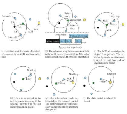
The aggregation data exchanges occur after nodes in a cluster have received LBs from a location node (Figure 5(a)). For the aggregation data exchanges, reservable time slots are used. The time slots form an aggregation superframe as illus-trated inFigure 5(b). Each time slot is further divided into an uplink slot and a downlink slot. Reliable communication is enabled using MAC-level acknowledgments.
A synchronization mechanism is needed to correlate a time slot to a common time reference among the nodes. A receiver-based synchronization scheme, similar to reference
broadcast synchronization (RBS) [66], is used. Instead of
using explicit synchronization packets, LBs are exploited to achieve synchronization.
Upon receiving an LB, an ACH or a subnode has knowl-edge about the exact time the active period of the source location node ends. The location node active period end acts as a synchronization point as depicted inFigure 5(b). The aggregation superframe follows the active period of the location node.
The relay data exchanges after aggregation are illustrated in Figures5(c),5(d),5(e), and5(f). The protocol exploits the fact that the next hop node can overhear the acknowledg-ment sent to the current hop source node (similar reasoning
is made for CTS packets in MARCH protocol [67]). Thus,
to reduce signaling and latency, the acknowledgments are made dual-purpose. First, they are used to acknowledge received packets. Secondly, the current hop acknowledgment
is used to signal next hop node of upcoming communication (Figures5(c)and5(e)).
The relayed data is communicated on separate RF channels. This reduces the interference that the the relay process causes to the localization data-acquisition pro-cess. Furthermore, by randomizing the channel for every relay communication transaction separately, the
interfer-ence between different data relay flows is minimized. The
acknowledgments are sent on location channel, so that the next hop nodes are able to receive them during the normal operation of listening for possible LBs. The current acknowledgment contains the randomized RF channel, the next hop node ID, and the exact time for next data relay transmission. Thus, the next hop node knows when to start listening in a correct channel.
3.2.4. Problematic situations
To make the channel access robust, the following problematic situations need to be addressed:
(i) an ACH does not hear any LB, but its members do,
(ii) subnodes belonging to the same cluster hear LBs from different location nodes, and
(iii) acknowledgment packets collide.
The first situation is resolved by using the location channel for aggregation data exchanges. If an ACH does not hear an LB, it cannot infer a synchronization point. Nevertheless, since all idle time is spent listening on the location channel, the relayed frames can be received.
The second situation introduces collisions, if two or more location nodes have active periods temporally close to each other. If subnodes fail to successfully transmit data in the reserved time slots, they try to retransmit the frames using slotted ALOHA [68].
If an acknowledgment packet is lost, the next hop node cannot receive the corresponding relay packet. In this
situation, the sender backs offfor a random amount of time
and tries to resend. The retransmission is signaled using an explicit RTS packet, which includes the same next hop information as an acknowledgment would.
4. LOCATION RESOLVER ALGORITHM
The presented location resolver algorithm follows the same principal idea as cell identification (CI) in cellular networks. In cellular networks, mobile stations (MSs) try to connect to a base station (BS) nearest to them. Thus, the MSs can infer their location to be somewhere in the coverage area of the BS in question [3].
Subnode
Subnode LB
LB LB
ACH Sink
(a) Location node transmits LBs, which are received by an ACH and two subn-odes
Relay-slot 0
Aggregation
Active periodSlot 0 Slot 1 Slotn Uplink Downlink Sync point
Relay-slot 1
Aggregation superframe (b) The subnodes relay the measurement data to the ACH they are associated to. After relay data reception, the ACH performs aggregation
ACK2 ACK1
ACK1,2 Next hop
(c) The ACH acknowledges the relayed data packets. The ac-knowledgements simultaneous-ly signal the next hop node of upcoming data packet
Relay Next hop
(d) The data is relayed to the next hop node according to the schedule informed in the last acknowledgement packet
ACK ACK
Next hop
(e) The intermediate node ac-knowledges the received packet. The acknowledgement simultane-ously signals the sink of upcoming data packet
Relay
Next hop
(f) The data packet is relayed to the sink
Figure5: Localization data aggregation and relay via multiple hops to the sink.
4.1. Location resolution using bounding boxes
Our scheme uses an approach, where an anchor node radio range with a certain transmission power is considered as a cell. Furthermore, variable transmission powers are used to introduce variable sized cells. The used algorithm tries to find out the minimum area that is bounded by the overlapping minimum-sized cells. To simplify calculations without considerably degrading the accuracy, the cells are modeled to be squares.
Figure 6 depicts three anchor nodes and one location
node. The anchor nodes can hear the location node with powersP1,P2, andP3, which map to radio rangesr1,r2, and r3, respectively. Furthermore, the radio ranges map to radio
coverage circles and square localization cells (LCs). A square can be fully determined by giving the coordinates of its bottom left and top right corners; LCn= {Pbl LC(n),Ptr LC(n)}.
The set of LCs used in one location estimation is denoted by LCS. In order to find the final bounding box (FBB) containing the location node, the intersection of LCs in one LCS needs to be determined. FBB is given by
FBB=
LCn∈LCS
LCn. (7)
Equation (7) can be solved by a lightweight algorithm
called min-max [69–71]. Min-max relies on the fact that
the intersection of all LCs can be acquired by taking the maximum of all coordinate minimums and the minimum of all maximums:
FBB=maxXbl
, maxYbl
,minXtr
, minYtr ,
(8)
whereXblis the set of bottom leftx-coordinates,Yblis the
set of bottom lefty-coordinates,Xtris the set of top right
x-coordinates, andYtr is the set of top righty-coordinates in
LCs contained by LCS.
4.2. Learning-based transmission power to range mapping
The raw input data for the localization procedure consists of a set of tuples in the form of pi,Pi j, where pi is the
position of an anchor node i and Pi j is the transmission
power of the minimum power LB received by an anchor node
iand sent by a location node j. The determination of LCs,
which are needed by the bounding box algorithm, requires
r1< r2< r3
r1
r2
r3 Final
bounding box
Approximated square cell Idealized radio
coverage with powerP3
Anchor node Location node
Figure6: Localization cells and final bounding box.
ranges (ri j). Usually, an initial calibration and measurements are required in the network setup phase to find out the relationship between RF-power and range. At fixed location, the signal strength received from an anchor node changes with time [15], implying the need for recurrent calibrations [11,16].
We acknowledge that also our location estimation algorithm would benefit from the calibration procedure. However, in order to achieve easy deployment and robust operation in changing conditions, it is not used. Instead, we introduce an algorithm called learning-based transmission power to range mapping. It corrects initial approximated ranges at run time and considers local environmental and RF propagation properties automatically.
Simplified indoor path loss models follow two basic approaches. In the first scheme, an explicit attenuations for every wall is added and the path loss between walls is treated as free-space path loss. Alternatively, the attenuation caused by walls is added implicitly by changing the path loss exponent (e) value. Since our algorithm has no knowledge of the environment and the obstacles contained by it a priori, we have adopted the varying path loss exponent approach.
Learning-based transmission power to range mapping is based on iterative bounding boxestechnique. Initially, an approximated path loss exponent value is used. Now, if the real path loss exponent is smaller than the approximated one, the bounding boxes do not necessarily overlap. This situation is depicted in Figure 7(a), wherer(P,e) gives the
range with transmission powerPand path loss exponente.
The iterative bounding boxes algorithm decrements the path loss exponent (and increments range) until all the bounding boxes in the calculation overlap and a valid result is obtained.
This is illustrated in Figure 7(b). The resolved path loss
exponent value is saved and can be used in future location resolutions.
If a situation where bounding boxes do not overlap is met again, the iterative bounding boxes algorithm is triggered
starting with the current path loss exponent value. This enables the maintenance of the path loss exponent giving the “worst case” LCs, without excessive runs of the iterative algorithm.Figure 8illustrates the relation of the worst case LC to the ideal and real radio coverage. The use of the worst case LC guarantees that the resolved FBB contains the location node. In order to avoid using the worst case path loss exponent value all the time, it can be reset to its initial value periodically. This way temporal changes in the environment can be taken into account.
Iterative bounding boxes increase the processing over-head compared to the simple bounding boxes algorithm, sincer(P,e) needs to be repeatedly calculated. Fortunately, the processing cost is amortized, since after a valid path
loss exponent is solved, a pair Pi,ri has been found.
This reduces the rest of the transmission power to distance mapping procedures to simple array indexing operations usingPias the key.
5. LOCALIZATION DATA ACQUISITION
PERFORMANCE ANALYSIS
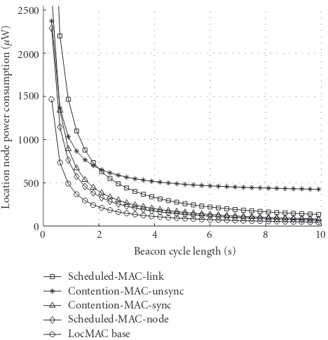
In this section, we will first compare the energy-efficiency of LocMAC base against low-power WSN MAC protocols.
Then, LocMAC base collision avoidance effectiveness is
evaluated using Matlab simulations.
5.1. Localization data acquisition energy-efficiency comparison
The related low-power MAC protocols are represented by four ideal protocol models; two contention-based and two schedule-based. First, models applicable for static networks are defined. Then, the models are complemented with neighbor discovery, which is needed when nodes are mobile. Our scheme is primarily targeted for very simple node HW using a radio transceiver not including RSSI support. This would make the usage of MAC protocols dependant on RSS infeasible. Nevertheless, they are also included to the comparison for thoroughness.
5.1.1. Derivation of MAC protocol models
The first contention-based protocol model, referred to as contention-MAC-unsync, represents low duty-cycle random-access MAC protocols. Energy unconstrained
anchor nodes can listen continuously to potential
uplink traffic (excluding the time they send packets).
Thus, a preamble of extended length is redundant when transmitting uplink and nonpersistent CSMA can be used.
For energy-efficient downlink communication,
contention-MAC-unsync uses LPL. A location node beacon cycle using
contention-MAC-unsync is illustrated inFigure 9.
r11=r(P1,e1)
r21=r(P2,e1)
(a)Bounding boxes with initial path loss exponent
r12=r(P1,e2)
r22=r(P2,e2)
(b) Bounding boxes with final path loss exponent Figure7: Iterative bounding boxes.
Real radio coverage
Idealized radio coverage
Approximated square cell using maximum
real radio range
Figure8: Worst-case localization cell.
Broadcast LBs
CCA Channel poll Beacon cycle
RX TX Location
node
LB4 LB3 LB2 LB1
Figure 9: Location node beacon cycle using contention-MAC-unsync.
node beacon cycle using contention-MAC-sync is illustrated
inFigure 10.
The first schedule-based protocol, referred to as sched-uled-MAC-link, uses TDMA with link activation. slot assign-ment scheme. Link activation does not enable the usage any single time slot for broadcast purposes. Broadcast has to be established as a series of unicasts as depicted in
Figure 11. Thus, the cost of transmitting LBs and listening for
downlink data is multiplied by the amount of synchronized neighbors. (There are two commonly used TDMA slot
Broadcast LBs CCA
Listen period Beacon cycle
RX TX Location
node
LB4 LB3 LB2 LB1
Figure 10: Location node beacon cycle using contention-MAC-sync.
allocation schemes referred to as node activation and link
activation [54]. In node activation slots are assigned to
individual nodes. Link activation assigns slots to links. Node activation allows efficient broadcast, since a node is able to transmit to any of its neighbors in its allocated slot. Nodes are not allowed to transmit simultaneously to neighbors that are not common to them even if this would not result in a collision. Link activation presents same properties in reversed order.) The second schedule-based protocol, referred to as scheduled-MAC-node, utilizes TDMA with node activation slot assignment scheme. As can be seen from
Figure 12, an LB broadcast reserves only one time slot. The
downlink slot amount is still proportional to the amount of synchronized neighbors.
5.1.2. power consumption models
Next, power consumption expressions for a location node using unsync, contention-MAC-sync, scheduled-MAC-link, scheduled-MAC-node, and Loc-MAC base are derived. The used symbols, their descriptions, and defined values are summarized inTable 1. Typical values
for IEEE.802.15.4 compliant radio (Chipcon CC2420 [72])
and the radio used in our prototype platforms (Nordic
Table1: Symbols, descriptions, and defined values for MAC power consumption analysis.
Symbol Description CC2420 nRF24L01
Ptx(n)n=4 Power in transmission mode at 0 dBm 52.2 mW 33.9 mW
Ptx(n)n=3 Power in transmission mode at−7/−6 dBm 37.5 mW 27 mW
Ptx(n)n=2 Power in transmission mode at−15/−12 dBm 29.7 mW 22.5 mW
Ptx(n)n=1 Power in transmission mode at−25/−18 dBm 25.5 mW 21 mW
Prx Power in reception 56.4 mW 35.4 mW
Psleep Power in sleep mode 60μW 2.7μW
tst Sleep to idle transient time 1.162 ms (measured) 1.63 ms
trssi RSSI average time 128μs —
Tbc Beacon cycle period Varying —
Tpoll Channel polling period 200 ms —
R Data rate 250 kbps 1/2 Mbps
Lf Frame length 256 bits 256 bits
Nnbor Number of one-hop neighbors (anchor nodes in radio range)a 3 —
Nlb Number of location beacons in one beacon set 4 —
aGenerally, at least three reference points is needed to achieve an unambiguous 2D location point estimate. Thus, three nodes per maximum transmission coverage area is used as the basis for anchor node density.
Communication with nodeX
Communication with nodeY Downlink time slot-unicast
Beacon cycle
Uplink time slots-unicast RX
TX Location
node
LB4
· · ·
LB1
Figure11: Location node beacon cycle using scheduled-MAC-link.
For simplicity and in order to ignore application-specific quantities it is assumed that (1) there is no downlink communication to the location node, but the protocol has to support it, (2) there are neither collisions nor retrans-missions, and (3) the clocks are perfectly synchronized, removing the need for reception margins. Furthermore, only radio energy consumption is considered (the energy consumption in WSN nodes is typically dominated by the radio transceiver circuitry [74]).
A frame transmission consists of a radio start-up tran-sient time (tst) and the time required by the actual data
transmission defined as the ratio of frame length (Lf) and radio data rate (R). During the start-up transient, the power consumption is estimated to be equal to the transmission mode powerPtx(n). Thus, the energy consumption (Etx(n)) of
a frame transmitted using a power levelnis
Etx(n)=
tst+ Lf
R
Ptx(n). (9)
A frame reception begins with the radio start-up tran-sient and lasts until the frame has been completely received. During a frame reception, the power consumption is equal to
the reception mode powerPrx. The frame reception energy
(Erx) is
Erx=
tst+ Lf
R
Prx. (10)
Since there are no reception margins, both successful and unsuccessful frame receptions consume energy equal toErx.
Total time required by one carrier sense operation is the sum of a radio start-up transient and the RSSI measurement
duration (trssi). Carrier sensing power is equal to the
reception-mode power. Thus, the carrier sensing energy (Ecs)
is
Ecs=
tst+trssi
Prx. (11)
LBs are transmittedNlbtimes using power levels ranging
from 1 toNlb. Prior to every transmission,
contention-MAC-unsync has to perform CCA, which consumes energy equal to carrier sensing (Ecs). The rest of the time, the channel is
polled atTpoll intervals, each poll consuming energy equal
toEcs. Since the transmission of a beacon set consists ofNlb
CCA operations, each having duration (tst+trssi), and LB
transmissions, each having duration (tst+Lf/R), the amount of channel polls (Npoll) in one beacon cycle (Tbc) is
Npoll=
Tbc−Nlb
2tst+trssi+Lf/R
Tpoll
. (12)
The total energy (Ebc contention unsync) consumed by
con-tention-MAC-unsync during one beacon cycle is
Ebc contention unsync=NlbEcs+
Nlb
n=1
To get the average power consumption (Pcontention unsync), the
total energy (Ebc contention unsync) consumed in one beacon
cycle is divided by the beacon cycle interval (Tbc):
Pcontention unsync=
Ebc contention unsync
Tbc .
(14)
Contention-MAC-sync transmits LBs similarly to
con-tention-MAC-unsync. For downlink traffic, the channel is
listened continuously for the duration of the listen period
tlisten. The listen period length is always the shortest possible.
Nodes sending downlink need to perform CCA prior to data transmission. Thus, minimum listen period energy is
Elisten=Nnbor
trssi+ Lf
R
Prx. (15)
The total energy consumption (Ebc contention sync) of
con-tention-MAC-sync during one beacon cycle is
Ebc contention sync=NlbEcs+
Nlb
n=1
Etx(n)+Elisten. (16)
The average power consumption (Pcontention sync) for
con-tention-MAC-sync is
Pcontention sync=
Ebc contention sync
Tbc . (17)
In scheduled-MAC-link, the beacon set is transmitted to every neighbor separately. Similarly, downlink slot needs to be received from every neighbor. Thus, the total energy consumption (Ebc scheduled link) during one beacon cycle is
Ebc scheduled link=Nnbor
Nlb
n=1
Etx(n)+Erx
. (18)
The average power consumption (Pscheduled link) for
sched-uled-MAC-link is
Pscheduled link= Ebc scheduled link
Tbc .
(19)
In scheduled-MAC-node, an LB is sent to all neigh-bors in a single time slot as illustrated in Figure 12. The downlink slot reception amount is still proportional to the neighbor count. The energy consumption (Ebc scheduled node)
of scheduled-MAC-node in one beacon cycle is
Ebc scheduled node=
Nlb
n=1
Etx(n)+NnborErx. (20)
The average power consumption (Pscheduled node) for
sched-uled-MAC-node is
Pscheduled node= Ebc scheduled node
Tbc .
(21)
The active period of LocMAC base is depicted in
Figure 13. Its energy consumption (Ebc locmac) is the sum of
the energies required by the transmission of the beacon set
Broadcast time slots Data from
nodeX
Data from nodeY Downlink
time slot Beacon cycle
RX TX Location
node
LB4
· · ·
LB1
Figure 12: Location node beacon cycle using scheduled-MAC-node.
Broadcast LBs
DL slot Beacon cycle
RX TX Location
node
LB4
· · ·
LB1
Figure13: LB transmissions with LocMAC.
and the reception of one downlink slot. Thus, the energy consumption of one beacon cycle is
Ebc locmac=
Nlb
n=1
Etx(n)+Erx. (22)
The corresponding average power consumption (Plocmac) is
Plocmac=Ebc locmac Tbc .
(23)
5.1.3. Neighbor discovery power consumption
Scheduled contention-access and TDMA-based low duty-cycle MAC protocols necessitate a neighbor discovery, when their neighborhood changes. In contrast, low duty-cycle random-access MACs, including LocMAC base, are typically able to broadcast packets without knowledge of their neigh-bors.
We divide neighbor discovery into initial and
mainte-nancediscoveries. An initial neighbor discovery is executed when a node has no known neighbors. This situation can occur at a boot-up, upon entering to the area of an WSN, or due to interference. Maintenance discovery is performed in order to maintain and update connectivity by establishing new links when new neighbors are encountered.
Table2: Additional symbols, descriptions, and defined values for neighbor discovery power consumption analysis.
Symbol Description Value
r Maximum radio range 10 m
ρ
Range of sufficient signal strength com-pared to maximum radio range with ENDP
0.5
fcb Cluster beacon transmission rate 0.5 Hz fnb Network beacon transmission rate 0.5 Hz fnbrx Network beacon reception rate 0.5 Hz
k
The amount of neighbors to which synchronization is maintained (equal Nnbor)
This kind of scenarios can result in large amounts of redundant initial neighbor discovery attempts, and high
energy consumption while being offline. To conserve energy,
the neighbor discovery period could be gradually increased after each initial neighbor discovery attempt. Yet, this would increase the latency of finding neighbors, when (re)entering the anchor WSN coverage area.
Secondly, location nodes can be highly mobile intro-ducing dynamics in the network. This sets stress on the maintenance neighbor discovery protocol. Thus, it can present significant energy overhead during online phase.
Next, we will derive models for neighbor discovery power consumption. Conventional network scanning is considered first. Then, neighbor discovery using ENDP follows. The
analysis utilizes symbols given in Table 1 and additional
symbols given inTable 2.
To make network scanning more energy-efficient, a
network beacon signaling scheme introduced in [21] is
used. A network-wide fixed channel is used to transmit network beacons containing node status information for the selection of an appropriate neighbor for association. The transmission of frequent network beacons reduces the energy
consumption in dynamic networks significantly [58]. The
beacons used for link establishment are referred to as cluster
beacons (the terminology used in [21] is adopted. Cluster
beacons do not necessarily imply the usage of clustered network topology). They contain information that is vital for data exchanges.
When a node moves out of its neighbors radio range (r), a link failure occurs. For a node moving at speedvand having links toNnbor nodes, the link failure rate (flf) can be
approximated to be [21]
flf= Nnborv
r . (24)
Nodes transmit network beacons with rate fnb. For
discovering all possible neighbors inside its radio range, a node needs to listen to the network channel for a whole network beacon period. Thus, the network scan duration is
tns=
1
fnb. (25)
In order to continuously maintain sufficient amount of
links, a mobile node needs to discover new neighbors at least every time a link is lost. Thus, using network scanning as neighbor discovery method, the scan interval (Tns) is
Tns=
1
flf.
(26)
The long-time average power consumed by network scanning in maintenance discovery is
Pns maintenance=
tst+tns
Prx
Tns .
(27)
Next, analytical expressions for neighbor discovery power consumption using ENDP are derived. To save space, a detailed derivation of the expressions is omitted. For more in-depth description of the derivation and equations, we refer the readers to [21].
ENDP can maintain links with proactive node schedule distribution as long as it receives valid synchronization data units (SDUs) from itskneighbors. After a link failure, a node tries to synchronize to neighbors using information provided by the SDUs. Synchronization is attempted until an attempt is successful, or all (k2) SDUs are examined. An invalid SDU
contains data about a node that is out of the radio range making synchronization to it impossible.
Assuming uniform node distribution, the probability (q) that the receivedk2SDUs fromkneighbors are invalid and a
network scan is required is
q=
k
a=1
1− Nnborpvalid Nnbor−(a−1)
k
, (28)
wherepvalid(≈59%) is the probability that the received SDU
is valid andadenotes the SDU index.
The probability of finding a neighbor in the first attempt is pvalid. If the attempt fails, the number of nodes outside
the radio range decreases. The expected number of network beacon receptions (u) until a neighbor inside the radio range is found is
u=pvalid+
k2−1
a=2
a a−1
b=1
1− Nnborpvalid Nnbor−(b−1)
N
nborpvalid Nnbor−(a−1)
+k2
k2−1
a=1
1− Nnborpvalid
Nnbor−(a−1)
.
(29)
When having no neighbors, a node needs to scan until a network beacon with sufficient signal strength is received.
The range of sufficient signal strength in proportion to
maximum radio range (r) is defined to beρ. Similarly to (29),
the expected number of network beacon receptions (Nnb)
until a beacon with sufficient signal strength is received is
Nnb=ρ2+
Nnbor−1
a=2
a a−1
b=1
1− Nnborρ
2
Nnbor−(b−1)
Nnborρ2 Nnbor−(a−1)
+Nnbor
Nnbor−1
a=1
1− Nnborρ2
Nnbor−(a−1)
.