Adaptive Rate Sampling and Filtering Based on Level Crossing Sampling

Volume 2009, Article ID 971656,12pages doi:10.1155/2009/971656

Research Article

Adaptive Rate Sampling and Filtering Based on

Level Crossing Sampling

Saeed Mian Qaisar,

_{Laurent Fesquet (EURASIP Member),}

_{and Marc Renaudin}

1_{TIMA, CNRS UMR 5159, 46 avenue Felix-Viallet, 38031 Grenoble Cedex, France}

2_{Tiempo SAS, 110 Rue Blaise Pascal, Bat Viseo-Inovallee, 38330 Montbonnot Saint Martin, France}

Correspondence should be addressed to Saeed Mian Qaisar,[email protected]

Received 11 August 2008; Revised 31 December 2008; Accepted 14 April 2009

Recommended by Sven Nordholm

The recent sophistications in areas of mobile systems and sensor networks demand more and more processing resources. In order to maintain the system autonomy, energy saving is becoming one of the most difficult industrial challenges, in mobile computing. Most of efforts to achieve this goal are focused on improving the embedded systems design and the battery technology, but very few studies target to exploit the input signal time-varying nature. This paper aims to achieve power efficiency by intelligently adapting the processing activity to the input signal local characteristics. It is done by completely rethinking the processing chain, by adopting a non conventional sampling scheme and adaptive rate filtering. The proposed approach, based on the LCSS (Level Crossing Sampling Scheme) presents two filtering techniques, able to adapt their sampling rate and filter order by online analyzing the input signal variations. Indeed, the principle is to intelligently exploit the signal local characteristics—which is usually never considered—to filter only the relevant signal parts, by employing the relevant order filters. This idea leads towards a drastic gain in the computational efficiency and hence in the processing power when compared to the classical techniques.

Copyright © 2009 Saeed Mian Qaisar et al. This is an open access article distributed under the Creative Commons Attribution License, which permits unrestricted use, distribution, and reproduction in any medium, provided the original work is properly cited.

1. Introduction

This work is part of a large project aimed to enhance the signal processing chain implemented in the mobile systems. The motivation is to reduce their size, cost, processing noise, electromagnetic emission and especially power consump-tion, as they are most often powered by batteries. This can be achieved by intelligently reorganizing their associated signal processing theory, and architecture. The idea is to combine event driven signal processing with asynchronous circuit design, in order to reduce the system processing activity and energy cost.

Almost all natural signals like speech, seismic, and biomedical are time varying in nature. Moreover, the man made signals like Doppler, Amplitude Shift Keying (ASK), and Frequency Shift Keying (FSK), also lay in the same category. The spectral contents of these signals vary with time, which is a direct consequence of the signal generation process [1]

The classical systems are based on the Nyquist signal processing architectures. These systems do not exploit the

signal variations. Indeed, they sample the signal at a fixed rate without taking into account the intrinsic signal nature. Moreover they are highly constrained due to the Shannon theory especially in the case of low activity sporadic signals like electrocardiogram, phonocardiogram, seismic, and so forth. It causes to capture, and to process a large number of samples without any relevant information, a useless increase of the system activity, and its power consumption.

Filtering is a basic operation, almost required in every signal processing chain. Therefore, this paper focuses on the development of efficient Finite Impulse Response (FIR) filtering techniques. The idea is to pilot the system processing activity by the input signal variations. By following this idea, an efficient solution is proposed by intelligently combining the features of both nonuniform and uniform signal process-ing tools, which promise a drastic computational gain of the proposed techniques compared to the classical one.

Section 2 briefly reviews the nonuniform signal pro-cessing tools employed in the proposed approach. Com-plete functionality of the proposed filtering techniques is described inSection 3.Section 4demonstrates the appealing features of the proposed techniques with the help of an illustrative example. The computational complexities of both proposed techniques are deduced and compared, among and to the classical case in Section 5. Section 6 discusses the processing error. InSection 7, the proposed techniques performance is evaluated for a speech signal.Section 8finally concludes the article.

2. Nonuniform Signal Processing Tools

2.1. LCSS (Level Crossing Sampling Scheme). The LCSS belongs to the signal-dependent sampling schemes like zero-crossing sampling [15], Lebesgue sampling [16], and reference signal crossing sampling [17]. The concept of LCSS is not new and has been known at least since 1950s [18]. It is also known as an event-based sampling [19, 20]. In recent years, there have been considerable interests in the LCSS, in a broad spectrum of technology and applications. In [21–24], authors have employed it for monitoring and control systems. It has also been suggested in literature for compression [2], random processes [25], and band-limited Gaussian random processes [26].

The LCSS is a natural choice for sampling the time-varying signals. It lets the signal to dictate the sampling process [4]. The nonuniformity in the sampling process represents the signal local variations [3]. In the case of LCSS, a sample is captured only when the input analog signalx(t) crosses one of the predefined thresholds. The samples are not uniformly spaced in time because they depend onx(t) variations as it is clear fromFigure 1.

Let a set of levels which span the analog signal amplitude range beΔVin.These levels are equally spaced by a quantum

q. Whenx(t) crosses one of these predefined levels, a sample is taken [2]. This sample is the couple (xn,tn) of an amplitude

xnand a timetn. Howeverxnis clearly equal to one of the

levels andtncan be computed by employing

tn=tn−1+dtn. (1)

In (1), tn is the current sampling instant, tn−1 is the previous one, anddtnis the time elapsed between the current

and the previous sampling instants.

2.2. LCADC (LCSS-Based Analog to Digital Converter). Clas-sically, during an ideal A/D conversion process the sampling instants are exactly known, where as samples amplitudes are

tn−1 tn dtn

q

t xn−1

xn x(t)

Figure1: Level-crossing sampling scheme.

quantized at the ADC resolution [27], which is defined by the ADC number of bits. This error is characterized by the Signal to Noise Ratio (SNR) [27], which can be expressed by

SNRdB=1.76 + 6.02M. (2) Here,Mis the ADC number of bits. It follows that the SNR of an ideal ADC depends only onMand it can be improved by 6.02 dB for each increment inM.

The A/D conversion process, which occurs in the LCADCs [7–9], is dual in nature. Ideally in this case, samples amplitudes are exactly known since they are exactly equal to one of the predefined levels, while the sampling instants are quantized at the timer resolutionTtimer. According to [7,8], the SNR in this case is given by

SNRdB=10 log

3Px

Px

−20 log(Ttimer). (3)

Here,PxandPxare the powers ofx(t) and of its derivative, respectively. It shows that in this case, the SNR does not depend onMany more, but onx(t) characteristics andTtimer. An improvement of 6.02 dB in the SNR can be achieved by simply halvingTtimer.

The choice ofM is however crucial. It should be taken large enough to ensure a proper reconstruction of the signal. This problem has been addressed in [28–31]. In particular, in [31], it is shown that a band-limited signal can be ideally reconstructed from nonuniformly spaced samples if the average number of samples satisfies the Nyquist criterion. In the case of LCADCs, the average sampling frequency depends onMand the signal characteristics [7–9]. Thus, for a given application an appropriateMshould be chosen in order to respect the reconstruction criterion [31].

In [7–9], authors have shown advantages of the LCADCs over the classical ones. The major advantages are the reduced activity, the power saving, the reduced electromagnetic emission, and the processing noise reduction. Inspiring from these interesting features, the Asynchronous Analog to Digital Converter (AADC) [7] is employed to digitize

produced by the AADC. We have already defined the AADC amplitude range ΔVin, the number of bits M and the quantumq. They are linked by the following relation:

q= ΔVin

2M₋₁. (4)

This quantum together with the AADC processing delay for one sampleδyields the upper limit on the input signal slope, which can be captured properly:

dx(t)

dt ≤ q

δ. (5)

In order to respect the reconstruction criterion [31] and the tracking condition [7], a band pass filter with pass-band [fmin;fmax] is employed at the AADC input. This together with a givenMinduces the AADC maximum and minimum sampling frequencies [6,11], defined by

Fsmax=2fmax

2M_{−1, (6)}

Fsmin=2fmin

2M−1. (7)

Here, fmax and fmin are the x(t) bandwidth and fun-damental frequencies, Fsmax and Fsmin are the AADC maximum and minimum sampling frequencies, respectively.

2.3. ASA (Activity Selection Algorithm). The nonuniformly sampled signal obtained with the AADC can be used for further nonuniform digital processing [3,10,13]. However in the studied case, the nonuniformity of the sampling process, which yields information on the signal local fea-tures, is employed to select only the relevant signal parts. Furthermore, the characteristics of each signal selected part are analyzed and are employed later on to adapt the proposed system parameters accordingly. This selection and local-features extraction process is named as the ASA.

For activity selection, the ASA exploits the information laying in the level-crossing sampled signal nonuniformity [5]. This selection process corresponds to an adaptive length rectangular windowing. It defines a series of selected windows within the whole signal length. The ability of activity selection is extremely important to reduce the pro-posed system processing activity and consequently its power consumption. Indeed, in the proposed case, no processing is performed during idle signal parts, which is one of the reasons of the achieved computational gain compared to the classical case. The ASA is defined as follow:

while

dtn≤T0

2 ,T

i_≤T

ref

Ti = Ti_+dt n;

Ni _{= N}i_{+ 1;}

end.

(8)

Here,dtnis clear from (1).T0 = 1/ fmin is the fundamental period of the bandlimited signal x(t),T0 and dtn detect

parts of the nonuniformly sampled signal with activity. If the measured time delay dtn is greater than T0/2,x(t) is considered to be idle. The conditiondtn ≤ T0/2 is chosen to ensure the Nyquist sampling criterion for fmin.

Tref is the reference window length. Its choice depends on the input signal characteristics and the system resources. The upper bound onTrefis posed by the maximum number of samples that the system can treat at once. Whereas the lower bound onTref is posed by the conditionTref ≥ T0, which should be respected in order to achieve a proper spectral representation [5].

Ti _{represents the length in seconds of the ith selected}

window Wi_{. T}

refposes the upper bound on Ti. Ni rep-resents the number of nonuniform samples laying in Wi_,

which lies on the jth active part of the nonuniformly sampled signal. i and j both belong to the set of natural numbersN∗_{. The jth signal activity can be longer thanT}

ref. In this case, it will be splitted into more than one selected windows.

The above-described loop repeats for each selected window, which occurs during the observation length ofx(t). Every time before starting the next loop,iis incremented and

Ni_andTi_{are initialized to zero.}

The maximum number of samplesNmax, which can take place within a chosenTrefcan be calculated by employing

Nmax=TrefFsmax. (9) The ASA displays interesting features, which are not available in the classical case. It only selects the active parts of the nonuniformly sampled signal. Moreover, it correlates the length of the selected window with the input signal activity, laying in it. In addition, it also provides an efficient reduction of the phenomenon of spectral leakage in the case of transient signals. The leakage reduction is achieved by avoiding the signal truncation problem with a simple and an efficient algorithm, instead of employing a smoothening (cosine) window function, which is used in the classical schemes [5]. These abilities make the ASA extremely effective in reducing the overall system processing activity, especially in the case of low activity sporadic signals [5,6,11,12,14].

3. Proposed Adaptive Rate Filtering

3.1. General Principle. Two techniques are described to filter the selected signal obtained at the ASA output. The signal processing chain common to both filtering techniques is shown inFigure 2.

The activity selection and the local features extraction are the bases of the proposed techniques. They make to achieve the adaptive rate sampling (only relevant samples to process) along with the adaptive rate filtering (only relevant operations to deliver a filtered sample). Such an achievement assures a drastic computational gain of the proposed filtering techniques compared to the classical one. The steps of realizing these ideas are detailed in the following subsections.

Adapted filter forWi

Filtered signal (yn) Adapted parameters

forWi Parameters

adaptor for Wi Reference parameters

Band pass filtered analog signalx(t)

Non-uniformly sampled signal

(xn,tn)

Local parameters

forWi

Uniformly sampled signal

(xrn,trn) Selected signal

(xs,ts)

AADC ASA Resampler

Figure2: Signal processing chain common to both filtering techniques.

follows that the local sampling frequencyFsi_{can be specific}

forWi_{. According to [5]Fs}i_{can be calculated by employing}

Fsi₌ Ni

Ti. (10)

The upper and the lower bounds on Fsi _{are posed}

by Fsmax and Fsmin, respectively. In order to perform a classical filtering algorithm, the selected signal laying inWi_is

uniformly resampled before proceeding to the filtering stage (cf.Figure 2). Characteristics of the selected signal part laying inWi_{are employed to choose its resampling frequencyFrs}i_.

Once the resampling is done, there areNri_{samples in W}i_.

Choice ofFrsi_{is crucial and this procedure is detailed in the}

following subsection.

3.1.2. Adaptive Rate Filtering. It is known that for fixed design parameters (cut-offfrequency, transition-band width, pass-band, and stop-band ripples) the FIR filter order varies as a function of the operational sampling frequency. For high sampling frequency, the order is high and vice versa. In the classical case, the sampling frequency and filter order both remains unique regardless of the input signal variations, so they have to be chosen for the worst case. This time invariant nature of the classical filtering causes a useless increase of the computational load. This drawback has been resolved up to a certain extent by employing the multirate filtering techniques [32–34].

The proposed filtering techniques of this paper are the intelligent alternatives to the multirate filtering techniques. They achieve computational efficiency by adapting the sampling frequency and the filter order according to the input signal local variations. Both techniques have some common features, which are described in the following.

In both cases, a reference FIR filter is offline designed for a reference sampling frequencyFref. Its impulse response is

hk, wherekis indexing the reference filter coefficients.Frefis chosen in order to satisfy the Nyquist sampling criterion for

x(t), namelyFref≥2fmax.

During online computation,Fref and the local sampling frequency Fsi _{of window W}i _{are used to define the local}

resampling frequency Frsi _{and a decimation factord}i_{. The}

Frsi _{is employed to uniformly resample the selected signal}

laying in Wi_{, where as d}i_{is employed to decimate h}

k for filteringWi_.

Frsi_{can be specific depending upon Fs}i _{[11, 12]. For}

proper online filtering, Frefand Frsi should match. The approaches of keepingFref andFrsi coherent are explained below.

In the case, when Fsi _{≥ F}

ref,Frsi = Fref is chosen and

hkremains unchanged. This case is treated similarly by both

proposed techniques. This choice ofFrsi_{makes to resample}

Wi _{closer to the Nyquist rate, so avoiding unnecessary}

interpolations during the data resampling process. It thus further improves the proposed technique computational efficiency. This case is included in the description (see flowcharts in Figures3and4) of the following two filtering techniques.

In the opposite case, that is, Fsi _{< F}

ref, Frsi = Fsi is chosen andhkis online decimated in order to reduceFrefto

Frsi_{. In this case, the reference filter order is reduced forW}i_,

which reduces the number of operations to deliver a filtered sample [6,11]. Hence, it improves the proposed techniques computational efficiency. In this case, it appears thatFrsi

may be lower than the Nyquist frequency ofx(t) and so it can cause aliasing. According to [6,11], if the local signal amplitude is of the order of the maximal rangeΔVin, then for a suitable choice ofM(application-dependent) the signal crosses enough consecutive thresholds. Thus, it is locally oversampled with respect to its local bandwidth and so there is no aliasing problem. This statement is further illustrated with the results summarized inTable 3.

In order to decimatehkthe decimation factordiforWi

is online calculated by employing

di= Fref

Frsi, (11)

di_{can be specific for each selected window depending upon}

Frsi_{. For an integral d}i _{both techniques decimate h} k in a

similar way. Thus, a test ondi_{is made by computingD}i ₌

floor(di_{) and verifying if(D}i _{= d}i_{). Here, floor operation}

delivers only the integral part ofdi_{. If the answer is yes, then}

hkis decimated withDi, the process is clear from

hij=hDi_k. (12)

Equation (12) shows that the decimated filter impulse response for theith selected windowhi

jis obtained by picking

every (Di_{)th coefficient from h}

k. Here, j is indexing the

decimated filter coefficients. If the order ofhkisP, then the

Fsi_{< F}

ref

Frsi_=Fsi

di_=F

ref/Frsi

Di_=floor(di₎ Frsi_=F

ref

hi j=hk

If no If yes

Di_=di

If no If yes

Frsi_=F

ref/Di hij=DihiDk

Figure3: Flowchart of the ARD.

Fsi_{< F}

ref

Frsi_=Fsi

di_=Fref/Frsi Di_=floor(di₎ Frsi_=F

ref

hi j=hk

If no If yes

Di_=di

If no If yes

hij=resample(hk@Frsi)

hi j=DihiDk

hij=dihij

Figure4: Flowchart of the ARR.

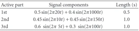
Table1: Summary of the input signal active parts.

Active part Signal components Length (s)

1st 0.5 sin(2π20t) + 0.4 sin(2π1000t) 0.5 2nd 0.45 sin(2π10t) + 0.45 sin(2π150t) 1.0 3rd 0.6 sin(2π5t) + 0.3 sin(2π100t) 1.0

A simple decimation causes a reduction of the decimated filter energy compared to the reference one. It will lead to an attenuated version of the filtered signal. Di_{is a good}

approximate of the ratio between the energy of the reference filter and that of the decimated one. Thus, this effect of decimation is compensated by scalinghi

jwithDi. The process

is clear from

hij=Di hDi_k. (13)

The two techniques mainly differ in the way of decimat-ing hk for a fractionaldi. The process is explained in the

following Sections.

3.2. ARD (Activity Reduction by Filter Decimation). In the ARD technique,hkis decimated by employingDi. It calls for

an adjustment ofFrsi_{which is achieved as Frs}i _{= F}

ref/Di. As in this case,Di_{< d}i_{, so it makesFrs}i_{> Fs}i_{. For the ARD}

hijscaling is performed withDi. The complete procedure of

obtainingFrsi_andhi

jfor the ARD is described inFigure 3.

3.3. ARR (Activity Reduction by Filter Resampling). In the ARR technique,di_{is employed to decimatedh}

k. In this case,

Frsi _{is given as Frs}i _{= F}

ref/di, so it remains equal to Fsi. The process of matchingFref withFrsi requires a fractional decimation ofhk, which is achieved by resamplinghkatFrsi.

Again NNRI is employed for the purpose ofhkresampling.

For the ARRhij scaling is performed withdi. The complete

procedure of obtainingFrsi_andhi

j for the ARR is described

inFigure 4.

4. Illustrative Example

In order to illustrate the ARD and the ARR filtering techniques, an input signal x(t) shown on the left part of Figure 5is employed. Its total duration is 20 seconds and it consists of three active parts. Summary ofx(t) activities is given inTable 1.

Table 1 shows thatx(t) is band limited between fmin =

5 Hz and fmax = 1 kHz. In this case, x(t) is digitized by

employing a 3-bit resolution AADC. Thus, for given ENOB the corresponding minimum and maximum sampling fre-quencies areFsmin=70 Hz andFsmax=14 kHz. The AADC

amplitude range ΔVin =1.8 v is chosen, which results into

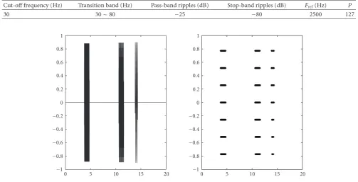
Table2: Summary of the reference filter parameters.

Cut-offfrequency (Hz) Transition band (Hz) Pass-band ripples (dB) Stop-band ripples (dB) Fref(Hz) P

30 30∼80 −25 −80 2500 127

0 5 10 15 20

−1

−0.8

−0.6

−0.4

−0.2 0 0.2 0.4 0.6 0.8 1

0 5 10 15 20

−1

−0.8

−0.6

−0.4

−0.2 0 0.2 0.4 0.6 0.8 1

Figure5: The input signal (left) and the selected signal obtained with the ASA (right).

Table3: Summary of the selected windows parameters.

i Ti_{(Sec.) N}i_{(Samples) Fs}i_{(Hz) F}

ref(Hz) Frsi(Hz) di

1 0.4994 3000 6000 2500 2500 1

2 0.9993 1083 1083 2500 1083 2.3

3 0.9986 464 464 2500 464 5.4

Each activity contains a low- and a high-frequency component (cf. Table 1). In order to filter out the high-frequency parts from each activity, a low pass reference FIR filter is implemented by employing the standard Parks-McClellan algorithm. The reference filter parameters are summarized inTable 2.

For this example the reference window length Tref = 1 second is chosen. It satisfies the boundary conditions discussed in Section 2.3. The given Tref delivers Nmax = 14000 samples in this case (cf. Equation (9)). The ASA delivers three selected windows for the wholex(t) span of 20 seconds, which are shown on the right part ofFigure 5. The selected windows parameters are displayed inTable 3.

Table 3shows that the first window is an example of the

Fsi _≥F

refcase, so it is tackled similarly by both techniques. In the other windows, Fsi _{< F}

refis valid, so the online

hk decimation is employed. As d2 and d3, calculated by

employing Equation (11) are fractional ones, so this case is tackled in a different way by the ARD and the ARR.

Values ofFrsi_,Di_,Nri_andPi_{are calculated for the ARD,}

and the ARR by employing the methods shown in Figures3 and4, respectively. The obtained results are summarized in Tables4and5.

Table4: Values ofFrsi_,Nri_,Di_{, and P}i_{for each selected window in}

the ARD.

i Frsi_{(Hz) Nr}i _Di _Pi

1 2500 1250 1 127

2 1250 1250 2 64

3 500 500 5 26

Tables3,4, and5jointly exhibit the interesting features of the proposed filtering techniques, which are achieved by an intelligent combination of the nonuniform, and the uniform signal processing tools (cf.Figure 2).Fsi_represents the sampling frequency adaptation by following the local variations of x(t).Ni _{shows that the relevant signal parts} are locally over-sampled in time with respect to their local bandwidths [6,11]. Frsi _{shows the adaptation of the} resampling frequency for each selected window. It further adds to the computational gain of the proposed techniques by avoiding the unnecessary interpolations during the resampling process.Nri _{shows how the adjustment of Frs}i avoids the processing of unnecessary samples during the post filtering process.Pi_{represents how the adaptation ofh}

k for Wi _{avoids the unnecessary operations to deliver the filtered} signal.Ti _{exhibits the dynamic feature of ASA, which is to} correlateTrefwith the signal activity laying in it [5].

Table5: Values ofFrsi_,Nri_,di_andPi_{for each selected window in the} ARR.

i Frsi_{(Hz) Nr}i _di _Pi

1 2500 1250 1 127

2 1083 1083 2.3 54

3 464 464 5.4 24

points is much lower, 3000 and 2794 for the ARD and the ARR, respectively. Moreover, the local filter orders inW2_and

W3_{are also lower than 127. It promises the computational} efficiency of the proposed techniques compared to the classical one. A detailed complexity comparison is made in the following Section.

5. Computational Complexity

In the classical case, with a Porder filter, it is well known that

P multiplications andP additions are required to compute each filtered sample. If N is the number of samples then the total computational complexityC can be calculated by employing

C= P N

Additions

+ P N

Multiplications

. (14)

In the adaptive techniques presented here, the adaptation process requires extra operations for each selected window. The computational complexities of both techniques, CARD andCARRare deduces as follow.

The following steps are common to both the ARD and the ARR techniques. The choice ofFrsi_{is a common operation}

for both proposed techniques. It requires one comparison betweenFrefandFsi. The data resampling operation is also required in both techniques before filtering. In the studied case, the resampling process is performed by employing the Nearest Neighbour Resampling Interpolation (NNRI). The NNRI is chosen because of its simplicity, as it employs only one nonuniform observation for each resampled one. Moreover, it provides an unbiased estimate of the original signal variance. Due to this reason, it is also known as a robust interpolation method [35,36]. The detailed reasons of inclination toward NNRI are discussed in [5,35,36]. The NNRI is performed as follow.

For each interpolation instanttrn, the interval of

nonuni-form samples [tn,tn+1], within whichtrnlies is determined.

Then the distance oftrnto eachtnandtn+1is computed and a comparison among the computed distances is performed to decide the smaller among them. ForWi_{, the complexity}

of the first step isNi_+Nri_{comparisons and the complexity}

of the second step is 2Nri _{additions andNr}i_comparisons.

Hence, the NNRI total complexity for Wi _{becomes N}i ₊

2Nri_{comparisons and 2Nr}i_additions.

In the case, when Fsi _{< F}

re f, the decimation of hk

is performed in both techniques. In order to do so, di

is computed by performing a division between Fre f and

Frsi_{. D}i _{is calculated by employing a floor operation on}

di_{. A comparison is made between D}i _anddi_{. In the case}

whenDi _{= d}i_{, the process of obtaining h}i

j is similar for

both techniques (cf. Figures 3 and 4). In this case, the decimator simply picks every (Di_{)th coefficient from h}

k.

It has a negligible complexity compared to the operations like addition and multiplication. This is the reason why its complexity is not taken into account during the complexity evaluation process. In both techniques, the decimated filter impulse response is scaled, it requiresPi_{multiplications. The}

fractionaldi _{is tackled in a different way by each filtering}

technique and is detailed in the following subsections.

5.1. Complexity of the ARD Technique. Even ifdi_{is fractional}

in the case of ARD technique,hkdecimation is performed by

employingDi_.Frsi_{is modified in order to keep it coherent}

withFrefand it requires one division (cf.Figure 3). Finally, aPi_{-order filter performs P}i_Nri _{multiplications andP}i_Nri

additions for Wi_{. The combine computational complexity}

for the ARD techniqueCARDis given by

CARD=

I

i=1

α1 +β

Divisions + α

Floor

+Ni_+Nri_{+ 1 +α}

Comparisons

+Nri_Pi_{+ 2}

Additions

+Pi_Nri_+α

Multiplications

.

(15)

5.2. Complexity of the ARR Technique. In the case of ARR technique, di _{is employed as the decimation factor. The}

fractional decimation is achieved by resamplinghk atFrsi.

The resampling is performed by employing the NNRI, which performsP+2Pi_{comparisons and 2P}i_{additions to deliverh}i

j.

The remaining operation cost between the ARD and the ARR is common. The combine computational complexity for the ARR techniqueCARRis given by

CARR=

I

i=1

α

Divisions

+ α

Floor

+ Ni+Nri_{+ 1 +α1 +βP+ 2P}i

Comparisons

+Nri_Pi_{+ 2+ 2αβP}i

Additions

+Pi_Nri_+α

Multiplications

.

(16)

In Equations (15) and (16),i = 1, 2, 3,. . .,I, represents the selected windows index. α and β are the multiplying factors.αis 0 for the case whenFsi_≥F

refand it is 1 otherwise.

βis 0 for the case whendi_=Di_{and it is 1 otherwise.}

Table6: Computational gain of the ARD over the classical one for differentx(t) time spans.

Signal part Gain in additions Gain in multiplications

W1 _{1.98 2}

W2 _{3.91 3.96}

W3 _{23.51 24.37}

Whole signal 25.93 26.22

Table7: Computational gain of the ARR over the classical one for

differentx(t) time spans.

Signal part Gain in additions Gain in multiplications

W1 _{1.98 2}

W2 _{5.33 5.42}

W3 _{27.31 28.45}

Whole signal 29.44 29.81

the additions count and divisions plus floors are merged into the multiplications count, during the complexity evaluation process. Now Equations (15) and (16) can be written as follow:

CARD= I

i=1

Ni_+Nri_Pi_{+ 3+α+ 1}

Additions

+PiNri+αPi+ 2 +β

Multiplications

,

(17)

CARR= I

i=1

Ni_+Nri_Pi_{+ 3+α1 +βP+ 3P}i_{+ 1}

Additions

+PiNri+αPi+ 2

Multiplications

.

(18)

By employing results of the example studied in the previous section, computational comparisons of the ARD and the ARR with the classical one are made in terms of additions and multiplications. The results are computed for differentx(t) time spans and are summarized in Tables6and 7.

Gains in additions and multiplications of the proposed techniques over the classical one are clear from the above results. In the case ofW1_{, where the resampling frequency} and the filter order is the same as in the classical case (cf. Tables 4 and5), a gain is achieved by using the proposed adaptive techniques. This is only due to the fact that the ASA correlates the window length to the activity (0.5 second), while the classic case computes during the total duration of

Tre f = 1 second. Gains are of course much larger in other

windows, since the proposed techniques are taking benefit of processing the lesser samples along with the lower filter orders. When treating the whole x(t) span of 20 seconds, the proposed techniques also take advantage of the idlex(t) parts, which further induces additional gains compared to the classical case.

The above results confirm that the proposed filtering techniques lead toward a drastic reduction in the number of operations compared to the classical one. This reduction in operations is achieved due to the joint benefits of the AADC, the ASA and the resampling, as they enable to adapt the sampling frequency and the filter order by following the input signal local variations.

5.4. Complexity Comparison between the ARD and the ARR. The main difference between both proposed techniques occurs for the case whenFsi _{< F}

re f anddi is fractional (cf.

Section 3).

The ARD makes an increment inFrsi_{in order to keep it}

coherent withFre f. Increase in Frsi causes to increaseNri

and also to increase Pi_{. Thus, in comparison to the ARR,}

this technique increases the computational load of the post-filtering operation, while keeping the decimation process of

hksimple.

The ARR performs hk resampling at Frsi. Thus, in

comparison to the ARD, this technique increases the com-plexity of the decimation process of hk, while keeping the

computational load of the post-filtering process lower. In continuation toSection 5.3, a complexity comparison between the ARD and the ARR is made in terms of additions, and multiplications by employing Equations (17) and (18), respectively. It concludes that the ARR remains computationally efficient compared to the ARD, in terms of additions and multiplications, as far as the conditions given by expressions (19) and (20) remain true. Please note thatNri

andPi_{can be different for the ARD and the ARR (cf. Tables}

4and5):

Nri_Pi_{+ 3} ARD−

Nri_Pi_{+ 3} ARR>

P+ 3Pi ARR

(19)

Pi_Nri_{+ 1+ 1} ARD>

Pi_Nri_{+ 1}

ARR. (20)

For this studied example, d2 _andd3_{are fractional ones,} thus the ARD and the ARR proceed differently. Conditions (19) and (20) remain true for bothW2_andW3_{(cf. Tables4} and5). Hence, the gains in additions and multiplications of the ARR are higher than those of the ARD forW2_andW3_(cf. Tables6and7). It shows that except for very specific situation the ARR technique will always remain less expensive than the ARD. The ARR achieves this computational performance by employing the fractional decimation ofhk, which may lead a

quality compromise of the ARR compared to the ARD. This issue is addressed in the following section.

6. Processing Error

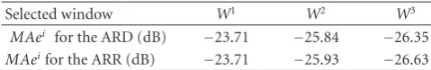
Table8: Mean approximation error of each selected window for the ARD and the ARR.

Selected window W1 _W2 _W3

MAei _{for the ARD (dB) −23.71 −25.84 −26.35}

MAei_{for the ARR (dB) −23.71 −25.93 −26.63}

two operations, the mean approximation error forWi_can

be computed by employing the following:

MAei= 1

Nri Nri

n=1

|xon−xrn|. (21)

Here,xrnis thenth resampled observation, interpolated with

respect to the time instanttrn,xonis the original sample value

which should be obtained by sampling x(t) at trn. In the

studied example discussed in Section 4,x(t) is analytically known, thus it is possible to compute its original sample value at any given time instant. It allows us to compute the approximation error introduced by the proposed adaptive rate techniques by employing Equation (21).

The results obtained for each selected window for both the ARD and the ARR are summarized inTable 8.

Table 8shows the approximation error introduced by the proposed techniques. This process is accurate enough for a 3-bit AADC. For the higher precision applications, the approximation accuracy can be improved by increasing the AADC resolution M and the interpolation order [6,8,37, 38]. Thus, an increased accuracy can be achieved at the cost of an increased computational load. Therefore, by making a suitable compromise between the accuracy level and the computational load, an appropriate solution can be devised for a specific application.

For a givenMand interpolation order the approximation accuracy can be further improved by employing the symme-try during the interpolation process. It results into a reduced resampling error [38,39]. The pros and cons of this approach are under investigation and a description on it is given in [40].

6.2. Filtering Error. In the proposed filtering techniques, a reference filter hk is employed and then it is online

decimated forWi_{, depending on the chosenFrs}i_{. This online}

decimation can cause the filtering precision degradation. In order to evaluate this phenomenon on our test signal the following procedure is adapted.

A reference filtered signal is generated. In this case, instead of decimating hk to obtain hij, a specific filter him

is directly designed for Wi _{by using the Parks-McClellan}

algorithm. It is designed for Frsi _{by employing the same}

design parameters, summarized inTable 2. The signal activ-ity corresponding to Wi _{is sampled at Frs}i _{with a high}

precision classical ADC. This sampled signal is filtered by employinghi

m. The filtered signal obtained in this way is used

as a reference one forWi_{, and its comparison is made with}

the results obtained by the proposed techniques.

Let yn be the nth reference-filtered sample and yn be

thenth filtered sample obtained by one of the proposed

Table9: Mean filtering error of each selected window for the ARD

and the ARR.

Selected window 1st 2nd 3nd

MFei_{for the ARD (dB) −43.23 −39.45 −17.07} MFei_{for the ARR (dB) −43.23 −30.46 −11.60}

filtering techniques. Then, the mean filtering error forWi

can be calculated by employing

MFei= 1

Nri Nri

i=1

_{yn−yn. (22)}

The mean filtering error of both proposed techniques is calculated, for eachx(t) activity by employing (22). The results are summarized inTable 9.

Table 9 shows that the online decimation of hk in the

proposed techniques causes a loss of the desired filtering quality. Indeed, the filtering error increases with the increase in di_{. The measure of this error can be used to decide an}

upper bound todi _{(by performing an offline calculation),}

for which the decimated and the scaled filters provide results with an acceptable level of accuracy. The level of accuracy is application-dependent. Moreover, for high precision appli-cations, an appropriate filter can be online calculated for each selected window at the cost of an increased computational load. The process is clear from generating the reference filtered signalyn, discussed above.

Table 9 shows that MFE2 _{and MFE}3 _{for the ARR are} higher than that of the ARD. It is due to the fact of hk

resampling for the ARR to deliver h2

j andh3j. It makes to

employ the interpolated coefficients ofhk for filtering the

resampled data, lies in W2 _{and W}3_{, respectively, which} results in an increased filtering error of the ARR compared to the ARD. Similar toSection 6.1, this resampling error can also be reduced to a certain extent, by employing a higher order interpolator [37,38]. In conclusion, a certain increase in the accuracy can be achieved at a certain loss of the processing efficiency.

7. Speech Signal as a Case Study

In order to evaluate performances of the ARD and the ARR for real life signals, a speech signalx(t)shown onFigure 6(a) is employed. x(t) is a 1.6 second, [50 Hz; 5000 Hz] band-limited signal corresponding to a three-word sentence. The goal is to determine the pitch (fundamental frequency) of

x(t) in order to determine the speaker’s gender. For a male speaker, the pitch lies with the frequency range [100 Hz, 150 Hz], whereas for a female speaker, the pitch lies with the frequency range [200 Hz, 300 Hz] [41].

The reference frequency is chosen as Fref = 11.2 kHz, which is a common sampling frequency for speech. A 4-bit resolution AADC is used for digitizingx(t), and therefore we haveFsmin =1.5 kHz, andFsmax =150 kHz. The amplitude range is always set toΔVin=1.8 V, which leads to a quantum

0 0.5 1 1.5

−1

−0.5 0 0.5 1

(a)

0 0.5 1 1.5

−1

−0.5 0 0.5 1

Vowel “a”

(b)

0.86 0.88 0.9 0.92 0.94 0.96

−0.6

−0.4

−0.2 0 0.2 0.4

(c)

150 200 250 300

0.03 0.04 0.05 0.06

(d)

150 200 250 300

0.03 0.04 0.05 0.06

(e)

150 200 250 300

0.03 0.04 0.05 0.06

(f)

Figure6: On the top, the input speech signal (a), the selected signal with the ASA (b) and a zoom of the second window W2_{(c). On the}

bottom, a spectrum zoom of the filtered signal laying in W2_{obtained with the reference filtering (d), with the ARD (e) and with the ARR}

(f), respectively.

The studied signal is part of a conversation and during a dialog, the speech activity is 25% of the total dialog time [42]. A classical filtering system would remain active during the total dialog duration. The proposed LCSS-based filtering techniques will remain active only during 25% of the dialog time span, which will reduce the system power consumption. A speech signal mainly consists of vowels and conso-nants. Consonants are of lower amplitude compared to vowels [41, 43]. In order to determine the speakers pitch, vowels are the relevant parts of x(t). For q = 0.12 v, consonants are ignored during the signal acquisition process, and are considered as low amplitude noise. In contrast, vowels are locally over-sampled like any harmonic signal [6,10,11]. This intelligent signal acquisition further avoids the processing of useless samples, within the 25% of x(t) activity, and so further improves the proposed techniques computational efficiency.

In order to apply the ASA,Tref =0.5 seconds is chosen. It results in Nmax = TrefFmax = 75000 in this case (cf. Equation (9)). The ASA delivers three selected windows, which are shown on Figure 6(b). The parameters of each selected window are summarized inTable 10.

Although the consonants are partially filtered out during the data acquisition process, yet for proper pitch estimation, it is required to filter out the remaining effect of high frequencies still present inx(t). To this aim, a reference low pass filter is designed, with the standard Parks-McClellan algorithm. Its characteristics are summarized inTable 11.

Table10: Summary of the selected windows parameters.

Selected window Ti_{(Second) N}i_{(Samples) Fs}i_(Hz)

Wi _{0.2074 2360 11379}

W2 _{0.1136 347 3054}

W3 _{0.1210 265 2190}

To find the pitch, we now focus on W2_{, which} corre-sponds to the vowel “a”. A zoom on this signal part is plotted onFigure 6(c). The conditionFs2 _{≤ F}

refis valid, andd2 is fractional (cf. Equation (11)).Thus, the filtering process for each proposed technique will differ, which makes it possible to compare their performances. The values ofFrs2_,Nr2_,D2_, andP2_{for both techniques are given inTable 12.}

Computational gains of the proposed filtering techniques compared to the classical one are computed by employing Equations (14), (17), and (18). The results show 8.62 and 13.17 times gains in additions and 8.71 and 13.26 times gains in multiplications, respectively, for the ARD and the ARR, for

W2_{. It confirms the computational efficiency of the proposed} techniques compared to the classical one. It is gained firstly by achieving an intelligent signal acquisition and secondly by adapting the sampling frequency and the filter order by following the local variations ofx(t).

Once more the conditions (19) and (20) remain true for

Table11: Summary of the reference filter paramete 1

Cut-offfrequency (Hz) Transition band (Hz) Pass-band ripples (dB) Stop-band ripples (dB) Fref P(order)

300 300∼400 −25 −80 11.2 284

Table12: Values ofFrs2_,N2_,D2_{, andP}2_{for the ARD and the ARR.}

W2 Frs2(Hz) Nr2 D2 P2

ARD 3733 424 3 95

ARR 3054 347 3.7 77

Spectra of the filtered signal laying inW2_{, obtained with} the reference filtering (cf. Section 6.2), with the ARD and with the ARR techniques are plotted, respectively, on Figures 6(d),6(e), and6(f).

The spectra on Figure 6 show that the fundamental frequency is about 215 HZ. Thus, one can easily conclude that the analyzed sentence is pronounced by a female speaker. Although it is required to decimate the reference filter 3 times and 3.7 times, respectively, for the ARD and the ARR, yet spectra of the filtered signal, obtained with the proposed techniques are quite comparable to spectrum of the reference-filtered signal. It shows that even after such a level of decimation, results delivered by the proposed techniques are of acceptable quality for the studied speech application.

The above discussion shows the suitability of the pro-posed techniques for the low activity time-varying sig-nals like electrocardiogram, phonocardiogram, seismic, and speech. Speech is a common, and easily accessible signal. Therefore, the proposed techniques performance is studied for a speech application, though it can be applied to other appropriate real signals like electrocardiogram, phonocar-diogram, and seismic. The devised approach versatility lays in the appropriate choice of system parameters like the AADC resolution M, the distribution of level crossing thresholds, and the interpolation order. These parameters should be tactfully chosen for a targeted application, so that they ensure an attractive tradeoffbetween the system computational complexity and the delivered output quality.

8. Conclusion

Two novel adaptive rate filtering techniques have been devised. These are well suited for low activity sporadic signals like electrocardiogram, phonocardiogram and seismic sig-nals. For both filtering techniques, a reference filter is offline designed by taking into account the input signal statistical characteristics and the application requirements.

The complete procedure of obtaining the resampling frequency Frsi _{and the decimated filter coefficients h}i

j

for Wi _{is described for both proposed techniques. The}

computational complexities of the ARD and the ARR are deduced and compared with the classical one. It is shown that the proposed techniques result into a more than one-order magnitude gain in terms of additions and multiplications over the classical one. It is achieved due to the joint benefits of the AADC, the ASA and the resampling as they allow the

online adaptation of parameters (Fsi_,Frsi_,Ni_,Nri_,Di_{, and}

Pi_{) by exploiting the input signal local variations. It}

drasti-cally reduces the total number of operations and therefore, the energy consumption compared to the classical case.

A complexity comparison between the ARD and the ARR is also made. It is shown that the ARR outperforms the ARD in most of the cases. Performances of the ARD and the ARR are also demonstrated for a speech application. The results obtained in this case are in coherence with those obtained for the illustrative example.

Methods to compute the approximation and the filtering errors for the proposed techniques are also devised. It is shown that the errors made by the proposed techniques are minor ones, in the studied case. A higher precision can be achieved by increasing the AADC resolution and the interpolation order. Thus, a suitable solution can be proposed for a given application by making an appropriate tradeoffbetween the accuracy level and the computational load.

A detailed study of the proposed filtering techniques computational complexities by taking into account the real processing cost at circuit level is in progress. Future works focus on the optimization of these filtering techniques and their further employment in real life applications.

References

[1] S. C. Sekhar and T. V. Sreenivas, “Adaptive window zero-crossing-based instantaneous frequency estimation,” EURASIP Journal on Applied Signal Processing, vol. 2004, no. 12, pp. 1791–1806, 2004.

[2] J. W. Mark and T. D. Todd, “A nonuniform sampling approach to data compression,”IEEE Transactions on Communications, vol. 29, pp. 24–32, 1981.

[3] M. Gretains, “Time-frequency representation based chirp like signal analysis using multiple level crossings,” inProceedings of 15th European Signal Processing Conference (EUSIPCO ’07), pp. 2154–2158, Poznan, Poland, September 2007.

[4] K. M. Guan and A. C. Singer, “Opportunistic sampling by level-crossing,” inProceedings of IEEE International Conference on Acoustics, Speech and Signal Processing (ICASSP ’07), vol. 3, pp. 1513–1516, Honolulu, Hawaii, USA, April 2007.

[5] S. M. Qaisar, L. Fesquet, and M. Renaudin, “Spectral analysis of a signal driven sampling scheme,” in Proceedings of the 14th European Signal Processing Conference (EUSIPCO ’06), Florence, Italy, September 2006.

[6] S. M. Qaisar, L. Fesquet, and M. Renaudin, “Computationally efficient adaptive rate sampling and filtering,” inProceedings of 15th European Signal Processing Conference (EUSIPCO ’07), pp. 2139–2143, Poznan, Poland, September 2007.

[8] N. Sayiner, H. V. Sorensen, and T. R. Viswanathan, “A level-crossing sampling scheme for A/D conversion,” IEEE Transactions on Circuits and Systems II, vol. 43, no. 4, pp. 335– 339, 1996.

[9] F. Akopyan, R. Manohar, and A. B. Apsel, “A level-crossing flash asynchronous analog-to-digital converter,” inProceedings of the International Symposium on Asynchronous Circuits and Systems (ASYNC ’06), pp. 12–22, Grenoble, France, March 2006.

[10] F. Aeschlimann, E. Allier, L. Fesquet, and M. Renaudin, “Asynchronous FIR filters: towards a new digital processing chain,” in Proceedings of the International Symposium on Asynchronous Circuits and Systems (ASYNC ’04), vol. 10, pp. 198–206, Crete, Greece, April 2004.

[11] S. M. Qaisar, L. Fesquet, and M. Renaudin, “Adaptive rate filtering for a signal driven sampling scheme,” inProceedings of IEEE International Conference on Acoustics, Speech and Signal Processing (ICASSP ’07), vol. 3, pp. 1465–1468, Honolulu, Hawaii, USA, April 2007.

[12] S. M. Qaisar, L. Fesquet, and M. Renaudin, “Computationally efficient adaptive rate sampling and filtering for low power embedded systems,” inProceedings of the International Con-ference on Sampling Theory and Applications (SampTA ’07), Thessaloniki, Greece, June 2007.

[13] F. Aeschlimann, E. Allier, L. Fesquet, and M. Renaudin, “Spectral analysis of level crossing sampling scheme,” in Proceedings of the International Conference on Sampling Theory and Applications (SampTA ’05), Samsun, Turkey, July 2005. [14] S. M. Qaisar, L. Fesquet, and M. Renaudin, “An adaptive

resolution computationally efficient short-time Fourier trans-form,”Research Letters in Signal Processing, vol. 2008, Article ID 932068, 5 pages, 2008.

[15] F. E. Bond and C. R. Cahn, “On sampling the zeros of bandwidth limited signals,”IRE Transactions on Information Theory, vol. 4, pp. 110–113, 1958.

[16] K. J. Astrom and B. Bernhardsson, “Comparison of Riemann and Lebesgue sampling for first order stochastic systems,” in Proceedings of the 41st IEEE Conference on Decision and Control (CDC ’02), vol. 2, pp. 2011–2016, Las Vegas, Nev, USA, December 2002.

[17] I. Bilinskis,Digital Alias Free Signal Processing, John Wiley & Sons, New York, NY, USA, 2007.

[18] P. H. Ellis, “Extension of phase plane analysis to quantized systems,”IRE Transactions on Automatic Control, vol. 4, pp. 43–59, 1959.

[19] M. Lim and C. Saloma, “Direct signal recovery from threshold crossings,”Physical Review E, vol. 58, no. 5B, pp. 6759–6765, 1998.

[20] M. Miskowicz, “Asymptotic effectiveness of the event-based sampling according to the integral criterion,”Sensors, vol. 7, no. 1, pp. 16–37, 2007.

[21] K. J. Astrom and B. Bernhardsson, “Comparison of periodic and event based sampling for first-order stochastic systems,” inProceedings of IFAC World Congress, pp. 301–306, 1999. [22] M. Miskowicz, “Send-on-delta concept: an event-based data

reporting strategy,”Sensors, vol. 6, no. 1, pp. 49–63, 2006. [23] P. G. Otanez, J. R. Moyne, and D. M. Tilbury, “Using

deadbands to reduce communication in networked control systems,” inProceedings of the American Control Conference (ACC ’02), vol. 4, pp. 3015–3020, Anchorage, Alaska, USA, May 2002.

[24] S. C. Gupta, “Increasing the sampling efficiency for a control system,”IEEE Transactions on Automatic and Control, pp. 263– 264, 1963.

[25] I. F. Blake and W. C. Lindsey, “Level-crossing problems for random processes,”IEEE Transactions on Information Theory, pp. 295–315, 1973.

[26] M. Miskowicz, “Efficiency of level-crossing sampling for ban-dlimited Gaussian random processes,” inProceedings of IEEE International Workshop on Factory Communication Systems (WFCS ’06), pp. 137–142, Torino, Italy, June 2006.

[27] R. H. Walden, “Analog-to-digital converter survey and analy-sis,”IEEE Journal on Selected Areas in Communications, vol. 17, no. 4, pp. 539–550, 1999.

[28] M. A. Nazario and C. Saloma, “Signal recovery in sinusoid-crossing sampling by use of the minimum-negative con-straint,”Applied Optics, vol. 37, pp. 2953–2963, 1988. [29] M. Lim and C. Saloma, “Direct signal recovery from threshold

crossings,”Physical Review E, vol. 58, no. 5B, pp. 6759–6765, 1998.

[30] F. J. Beutler, “Error free recovery from irregularly spaced samples,”SIAM Review, vol. 8, pp. 328–335, 1996.

[31] F. Marvasti,Nonuniform Sampling Theory and Practice, Kluwer Academic/Plenum Publishers, New York, NY, USA, 2001. [32] M. Vetterli, “A theory of multirate filter banks,”IEEE

Transac-tions on Acoustics, Speech, and Signal Processing, vol. 35, no. 3, pp. 356–372, 1987.

[33] S. Chu and C. S. Burrus, “Multirate filter designs using comb filters,”IEEE Transactions on Circuits and Systems, vol. 31, no. 11, pp. 913–924, 1984.

[34] R. E. Crochiere and L. R. Rabiner, Multirate Digital Signal Processing, Prentice-Hall, Englewood Cliffs, NJ, USA, 1993. [35] S. de Waele and P. M. T. Broersen, “Time domain error

measure for resampled irregular data,” in Proceedings of the 16th IEEE Instrumentation and Measurement Technology Conference (IMTC ’99), vol. 2, pp. 1172–1177, Venice, Italy, May 1999.

[36] S. de Waele and P. M. T. Broersen, “Error measures for resam-pled irregular data,”IEEE Transactions on Instrumentation and Measurement, vol. 49, no. 2, pp. 216–222, 2000.

[37] F. Harris, “Multirate signal processing in communication systems,” in Proceedings of 15th European Signal Processing Conference (EUSIPCO ’07), Poznan, Poland, September 2007. [38] D. M. Klamer and E. Masry, “Polynomial interpolation of randomly sampled bandlimited functions and processes,” SIAM Journal on Applied Mathematics, vol. 42, no. 5, pp. 1004– 1019, 1982.

[39] F. B. Hildebrand,Introduction to Numerical Analysis, McGraw-Hill, Boston, Mass, USA, 1956.

[40] S. M. Qaisar, L. Fesquet, and M. Renaudin, “An improved quality adaptive rate filtering technique based on the level crossing sampling,” inProceedings of the World Academy of Science, Engineering and Technology, vol. 31, pp. 79–84, July 2008.

[41] L. R. Rabiner and R. W. Schafer,Digital Processing of Speech Signals, Prentice-Hall, Englewood Cliffs, NJ, USA, 1978. [42] P. G. Fontolliet, Syst`emes de T´el´ecommunications, Dunod,

Paris, France, 1983.