High-Resolution Source Localization Algorithm Based on the Conjugate Gradient

Volume 2007, Article ID 73871,9pages doi:10.1155/2007/73871

Research Article

High-Resolution Source Localization Algorithm Based on

the Conjugate Gradient

Hichem Semira,1_{Hocine Belkacemi,}2_{and Sylvie Marcos}2

1_{D´epartement d’´electronique, Universit´e d’Annaba, BP 12, Sidi Amar, Annaba 23000, Algeria}

2_{Laboratoire des Signaux et Syst`emes (LSS), CNRS, 3 Rue Joliot-Curie, Plateau du Moulon, 91192 Gif-sur-Yvette Cedex, France}

Received 28 September 2006; Revised 5 January 2007; Accepted 25 March 2007

Recommended by Nicola Mastronardi

This paper proposes a new algorithm for the direction of arrival (DOA) estimation ofPradiating sources. Unlike the classical subspace-based methods, it does not resort to the eigendecomposition of the covariance matrix of the received data. Indeed, the proposed algorithm involves the building of the signal subspace from the residual vectors of the conjugate gradient (CG) method. This approach is based on the same recently developed procedure which uses a noneigenvector basis derived from the auxiliary vectors (AV). The AV basis calculation algorithm is replaced by the residual vectors of the CG algorithm. Then, successive orthogo-nal gradient vectors are derived to form a basis of the sigorthogo-nal subspace. A comprehensive performance comparison of the proposed algorithm with the well-known MUSIC and ESPRIT algorithms and the auxiliary vectors (AV)-based algorithm was conducted. It shows clearly the high performance of the proposed CG-based method in terms of the resolution capability of closely spaced uncorrelated and correlated sources with a small number of snapshots and at low signal-to-noise ratio (SNR).

Copyright © 2007 Hichem Semira et al. This is an open access article distributed under the Creative Commons Attribution License, which permits unrestricted use, distribution, and reproduction in any medium, provided the original work is properly cited.

1. INTRODUCTION

Array processing deals with the problem of extracting infor-mation from signals received simultaneously by an array of sensors. In many fields such as radar, underwater acoustics and geophysics, the information of interest is the direction of arrival (DOA) of waves transmitted from radiating sources and impinging on the sensor array. Over the years, many approaches to the problem of source DOA estimation have been proposed [1]. The subspace-based methods, which re-sort to the decomposition of the observation space into a noise subspace and a source subspace, have proved to have high-resolution (HR) capabilities and to yield accurate es-timates. Among the most famous HR methods are MUSIC [2], ESPRIT [3], MIN-NORM [4], and WSF [5]. The per-formance of these methods however degrades substantially in the case of closely spaced sources with a small number of snapshots and at a low SNR. These methods resort to the eigendecomposition (ED) of the covariance matrix of the re-ceived signals or a singular value decomposition (SVD) of the data matrix to build the signal or noise subspace, which is computationally intensive specially when the dimension of these matrices is large.

matrix. The second one finds a vector which is orthogonal to the signal subspace directly from the signal matrix by com-puting a set of weights that minimizes the signal power of the array output. Both methods estimate the DOA in the same way as the classical MUSIC estimator. In [11], an adaptive al-gorithm using the CG with the incorporation of the spatially smoothing matrix has been proposed to estimate the DOA of coherent signals from an adaptive version of Pisarenko. In almost all research works, the CG has been used in a similar way to the ED technique in the sense that the objective is to find the noise eigenvector and to implement any subspace-based method to find the DOA of the radiating sources.

In this paper, the CG algorithm, with its basic version given in [12], is applied to generate a signal subspace basis which is not based on the eigenvectors. This basis is rather generated using the residual vectors of the CG algorithm. Then, using the localization function and rank-collapse cri-terion of Grover et al. in [13,14], we form a DOA estimator based on the collapse of the rank of an extended signal sub-space fromP+ 1 toP (whereP is the number of sources). This results in a new high-resolution direction finding tech-nique with a good performance in terms of resolution capa-bility for the case of both uncorrelated and correlated closely spaced sources with a small number of snapshots and at low SNR.

The paper is organized as follows. InSection 2, we in-troduce the data model and the DOA estimation problem. In Section 3, we present the CG algorithm. Our proposed CG-based algorithm for the DOA estimation problem fol-lowing the same steps in [13,14] is presented inSection 4. After simulations with comparison of the new algorithm to the MUSIC, ESPRIT, and AV-based algorithms inSection 5, a few concluding remarks are drawn inSection 6.

2. DATA MODEL

We consider a uniformly spaced linear array havingM om-nidirectional sensors receiving P (P < M) stationary ran-dom signals emanating from uncorrelated or possibly cor-related point sources. The received signals are known to be embedded in zero mean spatially white Gaussian noise with unknown varianceσ2_{, with the signals and the noise being} mutually statistically independent. We will assume the sig-nals to be narrow-band with center frequency ν0. The kth M-dimensional vector of the array output can be represented as

x(k)=

P

j=1

aθj

sj(k) +n(k), (1)

wheresj(k) is the jth signal, n(k) ∈ CM×1 is the additive noise vector, anda(θj) is the steering of the array toward di-rection θj that is measured relatively to the normal of the array and takes the following form:

aθj

=1,ej2πν0τj_,ej2π2ν0τj_{,. . .,e}j2π(M−1)ν0τjT_{, (2)}

whereτj = (d/c) sin(θj), withcandddesignating the sig-nal propagation speed and interelement spacing, respectively. Equation (1) can be rewritten in a compact form as

x(k)=A(Θ)s(k) +n(k) (3)

with

A(Θ)=aθ1

,aθ2

,. . .,aθP

,

s(k)=s1(k),s2(k),. . .,sP(k)

T ,

(4)

whereΘ=[θ1,θ2,. . .,θP]. We can now form the covariance matrix of the received signals of dimensionM×M

R=Ex(k)xH_(k)=A(Θ)R

sA(Θ)H+σ2I, (5) where (·)H _{and I denote the transpose conjugate and the} M×Midentity matrix, respectively.Rs=E[s(t)sH(t)] is the signal covariance matrix, it is in general a diagonal matrix when the sources are uncorrelated and is nondiagonal and possibly singular for partially correlated sources. In practice, the data covariance matrixRis not available but a maximum likelihood estimate R based on a finite numberK of data samples can be used and is given by

R= 1

K K

k=1

x(k)xH(k). (6)

3. CONJUGATE GRADIENT (CG) ALGORITHM

The method of conjugate gradients (CG) is an iterative inver-sion technique for the solution of symmetric positive definite linear systems. Consider the Wiener-Hopf equation

Rw=b, (7)

whereR ∈ CM×M _{is symmetric positive definite. There are} several ways to derive the CG method. We here consider the approach from [12] which minimizes the following cost function:

Φ(w)=wHRw−2 RebHw. (8)

Algorithm 1depicts a basic version of the CG algorithm.αiis the step size that minimizes the cost functionΦ(w),βi pro-vides R-orthogonality for the direction vectordi,gi is the residual vector defined as

g_i=b−Rw_i= −∇Φw_i (9)

with∇(Φ) denoting the gradient of functionΦandi denot-ing the CG iteration.

w0=0,d1=gcg,0=b,ρ0=gHcg,0gcg,0

fori=1 toDdo

vi=Rdi

αi=_dρHi−1 i vi

wi=wi−1+αidi

gcg,i=gcg,i−1−αivi

ρi=gHcg,igcg,i

βi= ρi

ρi−1 =

_gcg,i2

_gcg,

i−1 2

di+1=βidi+gcg,i

End for

Algorithm1: Basic conjugate gradient algorithm.

properties summarized as follows [12]:

(i) R-orthogonality or conjugacy with respect toRof the vectorsdi, that is,dHi Rdj=0, for alli=j,

(ii) the gradient vectors are mutually orthogonal, that is,

gH

cg,igcg,j=0, for alli=j, (iii)gH

cg,idj=0, for allj < i,

(iv) if the gradient vectorsgcg,i,i =0,. . .,D−1, are nor-malized, then the transformed covariance matrixTD =

GH_cg,DRGcg,D of dimensionD×Dis a real symmetric tridiagonal matrix;

(v)DD=span{d1,d2,. . .,dD}≡span{Gcg,D}≡KD(R,b), where KD_{(R,b) = span{[b,Rb,R}2_{b,. . .,R}D−1_{b]} is the} Krylov subspace of dimension D associated with the pair (R,b) [12].

AfterD iterations, the CG algorithm produces an iter-ative method to solve the reduced rank Wiener solution of (7). Note that the basic idea behind the rank reduction is to project the observation data onto a lower-dimensional sub-space (D < M), defined by a set of basis vectors [15]. It is then worth noting that other reduced rank solutions have been obtained via the auxiliary vectors-based (AV) algorithm and the powers ofR(POR) algorithm [15]. These algorithms the-oretically and asymptotically yield the same solution as the CG algorithm since they proceed from the same minimiza-tion criterion and the same projecminimiza-tion subspace [16]. How-ever, as the ways of obtaining the solution differ, these meth-ods are expected to have different performance in practical applications.

In the following, we propose a new DOA estimator from the CG algorithm presented above.

4. PROPOSED DOA ESTIMATION ALGORITHM

In this section, the signal model (1)–(5) is considered and an extended signal subspace of rankP+ 1 nonbased on the eigenvector analysis is generated using the same basis

proce-dure developed in the work of Grover et al. [13,14]. Let us define the initial vectorb(θ) as follows:

b(θ)= Ra(θ)

Ra(θ), (10)

wherea(θ) is a search vector of the form (2) depending on θ ∈ [−90◦, 90◦]. When the Psources are uncorrelated and θ=θjforj=1,. . .,P, we have

Raθj

=Es2j

M+σ2_aθ j

+ P

l=1;l=j Es2

l

aH_θ

l

aθj

aθl

. (11)

It appears thatb(θj) is a linear combination of theP sig-nal steering vectors and thus it lies in the sigsig-nal subspace of dimensionP. However, whenθ=θjforj∈ {1,. . .,P},

Ra(θ)=

P

j=1

Es2 j

aH_θ

j

a(θ)aθj

+σ2_{a(θ). (12)}

b(θ) is then a linear combination of theP+ 1 steering vectors{a(θ),a(θ1),a(θ2),. . .,a(θP)}and therefore it belongs to the extended signal subspace of dimensionP+ 1 which includes the true signal subspace of dimension P plus the search vectora(θ).

For each initial vector described above (10) and after per-formingPiterations (D=P) of the CG algorithm, we form a set of residual gradient vectors{gcg,0,gcg,1,. . .,gcg,P−1gcg,P} (all these vectors are normalized exceptgcg,P). Therefore, it can be shown (seeAppendix A) that if the initial vectorb(θ) is contained in the signal subspace, then the set of vectors

Gcg,P = {gcg,0,gcg,1,. . .,gcg,P−1}will also be contained in the column space ofA(Θ), hence, the orthonormal matrixGcg,P1 spans the true signal subspace forθ=θj,j=1, 2,. . .,P, that is,

span Gcg,P

≡span A(Θ) (13)

and the solution vectorw =R−1_{b=a(θ)/Ra(θ)also lies} in the signal subspace

w∈span gcg,0,gcg,1,. . .,gcg,P−1

. (14)

1_{If we perform an eigendecomposition of the tridiagonal matrixT}

P =

GH

cg,PRGcg,P, we haveTP =Pi=1λieieHi , then thePeigenvaluesλi,i =

1,. . .,P, ofTPare thePprincipal eigenvalues of the covariance matrixR,

and the vectorsyi=Gcg,Pei,i=1,. . .,P, (whereeiis theith eigenvector

ofT_Pandy_iare the Rayleigh-Ritz vectors associated withKD_{(R,b)) are}

Now, whenθ=θjfor j∈ {1,. . .,P},Gcg,P+12spans the ex-tended subspace yielding (seeAppendix A)

span Gcg,P+1

≡span A(Θ),a(θ). (15)

In this case,wis also in the extended signal subspace, that is,

w∈span gcg,0,gcg,1,. . .,gcg,P

. (16)

Proposition 1. AfterPiterations of the CG algorithm the

fol-lowing equality holds forθ=θj,j=1, 2,. . .,P:

gH

cg,P(θ)=0, (17)

wheregcg,Pis the residual CG vector left unnormalized at itera-tionP.

Proof. Since the gradient vectors gcg,i generated by the CG algorithm are orthogonal [12], span{gcg,0,gcg,1,. . .,gcg,P}is of rankP+ 1. Using the fact that whenθ=θj,j=1, 2,. . .,P,

span gcg,0,gcg,1,. . .,gcg,P−1

=span A(Θ). (18)

Then

span gcg,0,gcg,1,. . .,gcg,P−1,gcg,P

=span A(Θ),gcg,P

. (19)

From Appendix A, it is shown that each residual gradient vector generated by the CG algorithm when the initial vector is in the signal subspace span{A(Θ)}will also belong to the signal subspace. This is then the case forgcg,P. Therefore, the rank of span{gcg,0,gcg,1,. . .,gcg,P−1,gcg,P}reduces toP yield-ing that in this casegcg,Pshould be zero or a linear combina-tion of the other gradient vectors which is not possible since it is orthogonal to all of them.

In view ofProposition 1, we use the following localiza-tion funclocaliza-tion as defined in [14, equation (22)]:

PKθ(n)₌ 1 _gH

cg,P

θ(n)_G

cg,P+1

θ(n−1)2, (20)

whereGcg,P+1(θ(n)) is the matrix calculated at stepnby per-formingD = P iterations of the CG algorithm with initial

2_{We can show that the eigenvalues of the (P+ 1)×(P+ 1) matrixT} P+1= GH

cg,P+1RGcg,P+1(the last vectorgcg,Pis normalized) are{λ1,. . .,λP,σ2},

where the eigenvaluesλi,i=1,. . .,P, are thePprincipal eigenvalues ofR

andσ2_{is the smallest eigenvalue ofR. The firstPRR vectors from the set} yi=Gcg,P+1ei,i=1,. . .,P, are asymptotically equivalents to the principal

eigenvectors ofR[17], and the last (RR) vector associated toσ2_is

orthog-onal to the principal eigenspace (belonging to the noise subspace), that is,

yH

P+1A(θ)=0.

residual vectorgcg,0(θ(n))=b(θ(n)) as defined in (10), that is,

Gcg,P+1

θ(n)_=g cg,0

θ(n)_,g cg,1

θ(n)_{,. . .,g}

cg,P

θ(n) (21)

θ(n) _{=nΔwithn = 1, 2, 3,. . ., 180}◦_/Δ◦ _{andΔis the search}

angle step.

Note that the choice of using 1/gcg,P(θ(n))2as a local-ization function was first considered. Since the results were not satisfactory enough, (20) was finally preferred. Accord-ing to the modified orthonormal AV [16], the normalized gradient CG and the AV are identical because the AV recur-rence is formally the same as Lanczos recurrecur-rence [12]. Thus, if the initial vectorgcg,0 in CG algorithm is parallel to the initial vector in AV, then all successive normalized gradients in CG will be parallel to the corresponding AV vectors (see Appendix B). Let gav,i, i = 0,. . .,P −1, represent the or-thonormal basis in AV procedure and the last unormalized vectors bygav,P. Then, it is easy to show that the CG spectra are related to the AV spectra by

PKθ(n)_=c P

θ(n)2

×gH

av,p

θ(n)_g av,0

θ(n−1)2 +· · ·+cP

θ(n−1)2

×gHav,p

θ(n)_g

av,P

θ(n−1)2−1 ,

(22)

where

_cP

θ(n)₌ gcg,P

θ(n) _μP−1

θ(n)

αP

θ(n)

βP

θ(n), (23) the difference, therefore, between the AV [13,14] and CG spectra is the scalars |cP(θ(n))|2 calculated at steps n−1 andndue to the last basis vector that is unnormalized (see Appendix Bfor the details). It is easy to show that we can ob-tain a peak in the spectrum ifθ(n)_=θ

j,j=1,. . .,P, because the last vector in the basisgcg,P(θ(n)) = 0. However, when θ(n) _{= θ}

j, j = 1,. . .,P,gcg,P(θ(n)) is contained in the ex-tended signal subspace span{A(Θ),a(θ(n)_{)}and the} follow-ing relation holds:

span Gcg,P+1

θ(n−1)_{=span A(Θ),aθ}(n−1)_{. (24)}

We can note thatgH cg,P(θ

(n)_)G

cg,P+1(θ(n−1)) =0 except when

gcg,P(θ(n)) is proportional toa(θ(n)) anda(θ(n)) is orthogonal both toA(Θ) anda(θ(n−1)_{) which can be considered as a very} rare situation in most cases.

In real situations,Ris unknown and we use rather the sample average estimateR as defined in (6). From (20), it is clear that when θ(n) _{= θ}

j, j = 1,. . .,P, we will have

gH cg,P(θ

(n)_)G

cg,P+1(θ(n−1))not equal to zero but very small andPK(θ(n)_{) very large but not infinite.}

than MUSIC since the gradient vectors forming the signal subspace basis necessary to construct the pseudospectrum must be calculated for each search angle. The proposed al-gorithm is therefore interesting for applications where a very high resolution capability is required in the case of a small number of snapshots and a low signal-to-noise ratio (SNR). This will be demonstrated through intensive simulations in the next section. Also note that when the search angle area is limited, the new algorithm has a comparable computational complexity as MUSIC.

5. SIMULATION RESULTS

In this section, computer simulations were conducted with a uniform linear array composed of 10 isotropic sensors whose spacing equals half-wavelength. There are two equal-power plane waves arriving on the array. The internal noises of equal power exist at each sensor element and they are statis-tically independent of the incident signal and of each other. Angles of arrival are measured from the broadside direction of the array. First, we fix the signal angles of arrival at−1◦and 1◦and the SNR’s at 10 dB. InFigure 1, we examine the pro-posed localization function or pseudo-spectrum when the observation data recordK = 50 compared with that of the AV-based algorithm [13,14,18,19] and of MUSIC. The CG pseudo-spectrum resolves the two sources better than the AV algorithm where the MUSIC algorithm completely fails. No-tice that the higher gain of CG method is due to the factorcp which depends on the norm of the gradient.

In the following, in order to analyze the performance of the algorithms in terms of the resolution probability, we use the following random inequality [20]:

PKθm

−1

2

PKθ1

+PKθ2

<0, (25)

whereθ1andθ2are the angles of arrivals of the two signals andθmdenotes their mean.PK(θ) is the pseudo-spectrum defined in (20) as a function of the angle of arrivalθ.

To illustrate the performance of the proposed algorithm two experiments were conducted.

Experiment 1(uncorrelated sources). In this experiment, we consider the presence of two uncorrelated complex Gaussian sources separated by 3◦. In Figures 2 and 3, we show the probability of resolution of the algorithms as a function of the SNR (whenK=50) and the number of snapshots (with SNR =0 dB), respectively. For purpose of comparisons, we added the ESPRIT algorithm [3]. As expected, the resolution capability of all the algorithms increases as we increase the number of snapshotsK and the SNR. We also clearly note the complete failure of MUSIC as well as ESPRIT to resolve the two signals compared to the two algorithms CG and AV (Krylov subspace-based algorithms). The two figures show that the CG-based algorithms outperforms its counterparts in terms of resolution probability.

−80 −60 −40 −20 0 20 40 60 80

Angle of arrival (◦)

−40

−20 0 20 40 60 80 100 120

Gain

(dB)

CG AV MUSIC

Figure1: CG, AV, and MUSIC spectra (θ1= −1◦,θ2=1◦, SNR1=

SNR2=10 dB,K=50).

−10−8−6−4 −2 0 2 4 6 8 10 12 14 16 18 20 SNR (dB)

0 0.1 0.2 0.3 0.4 0.5 0.6 0.7 0.8 0.9 1

P

robabilit

y

o

f

resol

ution

CG AV

ESPRIT MUSIC

Figure2: Probability of resolution versus SNR (separation 3◦_,K= 50).

Experiment 2 (correlated sources). In this experiment, we consider the presence of two correlated random complex Gaussian sources generated as follows:

s1∼N

0,σ2 S

, s2=rs1+

1−r2_s

3, (26)

10 20 30 40 50 60 70 80 90 100 Number of snapshots

0 0.1 0.2 0.3 0.4 0.5 0.6 0.7 0.8 0.9 1

P

robabilit

y

o

f

resol

ution

CG AV

ESPRIT MUSIC

Figure 3: Probability of resolution versus number of snapshots (separation 3◦_{, SNR=0 dB).}

−10−8−6−4−2 0 2 4 6 8 10 12 14 16 18 20 SNR (dB)

0 0.1 0.2 0.3 0.4 0.5 0.6 0.7 0.8 0.9 1

P

robabilit

y

o

f

resol

ution

CG with F/B spatial smoothing CG

AV with F/B spatial smoothing AV

ESPRIT with F/B spatial smoothing ESPRIT

MUSIC with F/B spatial smoothing MUSIC

Figure4: Probability of resolution versus SNR (separation 3◦_,K= 50,r=0.7).

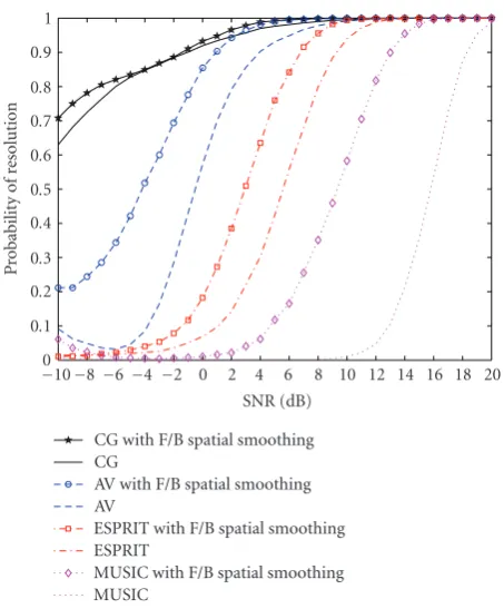
forward/backward spatial smoothing (FBSS) [21]. Figure 4 plots the probability of resolution versus SNR for a fixed record data K = 50 andFigure 5 plots the probability of resolution versus number of snapshots for an SNR = 5 dB. The two figures demonstrate that the CG-basis estimator still outperforms the AV-basis estimator in probability of

resolu-10 20 30 40 50 60 70 80 90 100

Number of snapshots 0

0.1 0.2 0.3 0.4 0.5 0.6 0.7 0.8 0.9 1

P

robabilit

y

o

f

resol

ution

CG with F/B spatial smoothing CG

AV with F/B spatial smoothing AV

ESPRIT with F/B spatial smoothing ESPRIT

MUSIC with F/B spatial smoothing MUSIC

Figure 5: Probability of resolution versus number of snapshots (separation 3◦, SNR=5 dB,r=0.7).

tion in the case of correlated sources with or without FBSS. We also note that the CG-based and the AV-based estimators (without FBSS) have better performance than MUSIC and ESPRIT with FBSS, at low SNR and whatever the record data size (Figure 5).

Finally, we repeat the previous simulations for highly cor-related sources (r =0.9). At low SNR (seeFigure 6), we show that the CG-based method even without FBSS still achieves better results than the AV-based method and over MUSIC and ESPRIT with or without FBSS (<8 dB for ESPRIT with spatial smoothing). InFigure 7, the proposed algorithm re-veals again higher performance over MUSIC and ESPRIT with or without FBSS; which is unlike its counterpart the AV-based algorithm where it has less resolution capability compared to ESPRTI with FBSS for data recordK <70. We can also notice the improvement of resolution probability for both the CG and AV-based algorithms with FBSS.

6. CONCLUSION

−10−8−6 −4 −2 0 2 4 6 8 10 12 14 16 18 20 SNR (dB)

0 0.1 0.2 0.3 0.4 0.5 0.6 0.7 0.8 0.9 1

P

robabilit

y

o

f

resol

ution

CG with F/B spatial smoothing CG

AVF with F/B spatial smoothing AVF

ESPRIT with F/B spatial smoothing ESPRIT

MUSIC with F/B spatial smoothing MUSIC

Figure6: Probability of resolution versus SNR (separation 3◦_,K= 50,r=0.9).

algorithm, the classical MUSIC and ESPRIT, in terms of res-olution capacity at a small record data and low SNR.

APPENDICES

A.

Let us assume thatb(θ)∈span{A(Θ),a(θ)}. It follows from Algorithm 1that

gcg,1=b(θ)−α1Rb(θ) (A.1) also belongs to span{A(Θ),a(θ)}since

Rb(θ)=

P

j=1

Es2 j

aθj

H

b(θ)aθj

+σ2_{b(θ) (A.2)}

is a linear combination of vectors of span{A(Θ),a(θ)}. Then

d2=gcg,1−β1d1also belongs to span{A(Θ),a(θ)}(withd1=

b(θ)). In the same way, we have

gcg,2=gcg,1−α2v2 (A.3) with

v2=Rd2 (A.4) also belonging to the extended signal subspace since

Rd2=

P

j=1

Es2j

aθj

H

d2(θ)

aθj

+σ2d2(θ). (A.5)

10 20 30 40 50 60 70 80 90 100

Number of snapshots 0

0.1 0.2 0.3 0.4 0.5 0.6 0.7 0.8 0.9 1

P

robabilit

y

o

f

resol

ution

CG with F/B spatial smoothing CG

AV with F/B spatial smoothing AV

ESPRIT with F/B spatial smoothing ESPRIT

MUSIC with F/B spatial smoothing MUSIC

Figure 7: Probability of resolution versus number of snapshots (separation 3◦, SNR=5 dB,r=0.9).

More generally, it is then easy to check that whengcg,i−1and

dcg,i−1are vectors of span{A(Θ),a(θ)}, thengcg,ianddcg,iare also vectors of span{A(Θ),a(θ)}. Now whenθ =θj, the ex-tended subspace reduces to span{A(Θ)}.

B.

Letgav,ibe the auxiliary vector (AV) [18,19]; it was shown in [16] that a simplified recurrence forgav,i+1,i≥1, is given by

gav,i+1=

I−i

l=i−1gav,lgav,Hl

Rgav,i

_I−i

l=i−1gav,lgav,Hl

Rgav,i

, (B.1)

gav,1=

Rgav,0−gav,0

gHav,0Rgav,0 _{Rgav,0−gav,0}

gHav,0Rgav,0

, (B.2)

wheregav,0is the first vector in the AV basis. Notice that the auxiliary vectors are restricted to be orthonormal in contrast to the nonorthogonal AV work in [19,22]. Recall that if ini-tial vectors are equals, that is,

gav,0=gcg,0=b(θ), (B.3)

then it is easy to show fromAlgorithm 1that

gcg,1

_gcg,1= − Rgcg,0−gcg,0

gHcg,0Rgcg,0 _{Rgcg,0−gcg,0}

gHcg,0Rgcg,0

From (B.1) we can obtain

tigav,i+1=Rgav,i−

gH

av,iRgav,i

gav,i−

gH

av,i−1Rgav,i

gav,i−1

δigav,i+1=Rgav,i−γigav,i−δi−1gav,i−1.

(B.5)

Thus, the last equation (B.5) is the well-known Lanczos re-currence [12], whereti = (I−

_i

l=i−1gav,lgav,Hl)Rgav,iand the coefficientsγiandδiare the elements of the tridiagonal matrixGH

av,iRGav,i, whereGav,iis the matrix formed by thei normal AV vectors. From the interpretation of Lanczos al-gorithm, if the initial gradient CG algorithmgcg,0is parallel to the initialgav,0, then all successive normalized gradients in CG are the same as the AV algorithm [12], that is,

gav,i=(−1)i

gcg,i

_gcg,i, i≥1. (B.6)

From the expression for the CG algorithm, we can express the gradient vectorsgcg,i+1in terms of the previous gradient vectors using line 6 and 9 ofAlgorithm 1, then we can write

gcg,i+1

αi+1 = −

Rgcg,i+

1 αi+1

+ βi αi

gcg,i−βi αi

gcg,i−1. (B.7)

Multiplying and dividing each term of (B.7) by the norm of the corresponding gradient vector results in [23]

βi+1

αi+1

gcg,i+1 _gcg,i+1

= −Rgcg,i gcg,i

+

1 αi+1

+βi αi

_g

cg,i

_gcg,i−

βi αi

gcg,i−1 _gcg,i−1.

(B.8)

If (B.8) is identified with (B.5), it yields

δi=

βi+1

αi+1 ,

γi= 1 αi+1

+βi αi

, i≥1,

γ1=gav,0H Rgav,0= 1 α1.

(B.9)

We will now prove the relation between the unormalized last vectorsgcg,Pandgav,P. From [13], the last unnormalized vec-tor in AV algorithm is given by

gav,P=(−1)P+1μP−1

I−

P−2

l=P−1

gav,lgHav,l

Rgav,P−1,

(B.10)

where

μi=μi−1

gHav,iRgav,i−1

gHav,iRgav,i

, i >1, (B.11)

μ1=

gHav,1Rgav,0

gHav,1Rgav,1.

(B.12)

Using (B.5) and (B.9), (B.12) can be rewritten as

μ1=δ1

γ2 =

β2

α2

1 α2

+ β1 α1

−1

(B.13)

and a new recurrence forμican be done with the CG coeffi -cients as

μi=μi−1

βi+1

αi+1

1 αi+1

+ βi αi

−1

, i >1, (B.14)

hence from (B.6), we can obtain

gcg,P=(−1)P

_{gcg,P μP−1}αP

βP

gav,P (B.15)

so the difference between the last unnormalized CG basis and the last unormalized AV basis is the scalar

cP=(−1)P

gcg,P

_μP−1αP βP

. (B.16)

ACKNOWLEDGMENT

The authors would like to express their gratitudes to the anonymous reviewers for their valuable comments, espe-cially the key result given in (22).

REFERENCES

[1] H. Krim and M. Viberg, “Two decades of array signal process-ing research: the parametric approach,”IEEE Signal Processing Magazine, vol. 13, no. 4, pp. 67–94, 1996.

[2] R. O. Schmidt, “Multiple emitter location and signal param-eter estimation,”IEEE Transactions on Antennas and Propaga-tion, vol. 34, no. 3, pp. 276–280, 1986.

[3] R. Roy and T. Kailath, “ESPRIT-estimation of signal param-eters via rotational invariance techniques,”IEEE Transactions on Acoustics, Speech, and Signal Processing, vol. 37, no. 7, pp. 984–995, 1989.

[4] R. Kumaresan and D. W. Tufts, “Estimating the angles of ar-rival of multiple plane waves,”IEEE Transactions on Aerospace and Electronic Systems, vol. 19, no. 1, pp. 134–139, 1983. [5] M. Viberg, B. Ottersten, and T. Kailath, “Detection and

esti-mation in sensor arrays using weighted subspace fitting,”IEEE Transactions on Signal Processing, vol. 39, no. 11, pp. 2436– 2449, 1991.

[6] H. Chen, T. K. Sarkar, S. A. Dianat, and J. D. Brule, “Adaptive spectral estimation by the conjugate gradient method,”IEEE Transactions on Acoustics, Speech, and Signal Processing, vol. 34, no. 2, pp. 272–284, 1986.

[8] P. S. Chang and A. N. Willson Jr., “Adaptive spectral estima-tion using the conjugate gradient algorithm,” inProceedings of IEEE International Conference on Acoustics, Speech, and Signal Processing (ICASSP ’96), vol. 5, pp. 2979–2982, Atlanta, Ga, USA, May 1996.

[9] Z. Fu and E. M. Dowling, “Conjugate gradient eigenstructure tracking for adaptive spectral estimation,”IEEE Transactions on Signal Processing, vol. 43, no. 5, pp. 1151–1160, 1995. [10] S. Choi, T. K. Sarkar, and J. Choi, “Adaptive antenna array

for direction-of-arrival estimation utilizing the conjugate gra-dient method,”Signal Processing, vol. 45, no. 3, pp. 313–327, 1995.

[11] P. S. Chang and A. N. Willson Jr., “Conjugate gradient method for adaptive direction-of-arrival estimation of coherent sig-nals,” inProceedings of IEEE International Conference on Acous-tics, Speech, and Signal Processing (ICASSP ’97), vol. 3, pp. 2281–2284, Munich, Germany, April 1997.

[12] G. H. Golub and C. F. V. Loan,Matrix Computations, Johns Hopkins University Press, Baltimore, Md, USA, 3rd edition, 1996.

[13] R. Grover, D. A. Pados, and M. J. Medley, “Super-resolution di-rection finding with an auxiliary-vector basis,” inDigital Wire-less Communications VII and Space Communication Technolo-gies, vol. 5819 ofProceedings of SPIE, pp. 357–365, Orlando, Fla, USA, March 2005.

[14] R. Grover, D. A. Pados, and M. J. Medley, “Subspace direction finding with an auxiliary-vector basis,”IEEE Transactions on Signal Processing, vol. 55, no. 2, pp. 758–763, 2007.

[15] S. Burykh and K. Abed-Meraim, “Reduced-rank adaptive fil-tering using Krylov subspace,”EURASIP Journal on Applied Signal Processing, vol. 2002, no. 12, pp. 1387–1400, 2002. [16] W. Chen, U. Mitra, and P. Schniter, “On the equivalence of

three reduced rank linear estimators with applications to DS-CDMA,” IEEE Transactions on Information Theory, vol. 48, no. 9, pp. 2609–2614, 2002.

[17] G. Xu and T. Kailath, “Fast subspace decomposition,”IEEE Transactions on Signal Processing, vol. 42, no. 3, pp. 539–551, 1994.

[18] D. A. Pados and S. N. Batalama, “Joint space-time auxiliary-vector filtering for DS/CDMA systems with antenna arrays,”

IEEE Transactions on Communications, vol. 47, no. 9, pp. 1406– 1415, 1999.

[19] D. A. Pados and G. N. Karystinos, “An iterative algorithm for the computation of the MVDR filter,”IEEE Transactions on Signal Processing, vol. 49, no. 2, pp. 290–300, 2001.

[20] Q. T. Zhang, “Probability of resolution of the MUSIC algo-rithm,”IEEE Transactions on Signal Processing, vol. 43, no. 4, pp. 978–987, 1995.

[21] S. U. Pillai and B. H. Kwon, “Forward/backward spatial smoothing techniques for coherent signal identification,”IEEE Transactions on Acoustics, Speech, and Signal Processing, vol. 37, no. 1, pp. 8–15, 1989.

[22] H. Qian and S. N. Batalama, “Data record-based criteria for the selection of an auxiliary vector estimator of the MMSE/MVDR filter,”IEEE Transactions on Communications, vol. 51, no. 10, pp. 1700–1708, 2003.

[23] D. Segovia-Vargas, F. I˜nigo, and M. Sierra-P´erez, “Generalized eigenspace beamformer based on CG-Lanczos algorithm,”

IEEE Transactions on Antennas and Propagation, vol. 51, no. 8, pp. 2146–2154, 2003.

Hichem Semirawas born on December 21, 1973 in Constantine, Algeria. He received the B.Eng. degree in electronics in 1996 and the Magist`ere degree in signal processing in 1999 both from Constantine University (Al-geria). He is now working towards Ph.D. degree in the Department of Electronics at Annaba University (Algeria). His research interests are in signal processing for com-munications, and array processing.

Hocine Belkacemi was born in Biskra, Algeria. He received the engineering de-gree in electronics from the Institut Na-tional d’Electricit´e et d’Electronique (IN-ELEC), Boumerdes, Algeria, in 1996, the Magist`ere degree in electronic systems from

´

Ecole Militaire Polytechnique, Bordj El Bahri, Algeria, in 2000, the M.S. (D.E.A.) degree in control and signal processing and the Ph.D. degree in signal processing both from

Uni-versit´e de Paris-SudXI, Orsay, France, in 2002 and 2006, respec-tively. He is currently an Assistant Teacher with the radio com-munication group at theConservatoire National des Arts et M´etiers CNAM, Paris, France. His research interests include array signal processing with application to radar and communications, adap-tive filtering, non-Gaussian signal detection and estimation.

Sylvie Marcosreceived the engineer degree from theEcole Centrale de Paris(1984) and both the Doctorate (1987) and the Habilita-tion(1995) degrees fromUniversit´e de Paris-Sud XI, Orsay, France. She isDirecteur de Rechercheat the National Center for Scien-tific Research (CNRS) and works in Lab-oratoire des Signaux et Syst`emes (LSS) at Sup´elec, Gif-sur-Yvette, France. Her main research interests are presently array