A Weberized Total Variation Regularization-Based Image Multiplicative Noise Removal Algorithm

Volume 2010, Article ID 490384,15pages doi:10.1155/2010/490384

Research Article

A Weberized Total Variation Regularization-Based Image

Multiplicative Noise Removal Algorithm

Liang Xiao, Li-Li Huang, and Zhi-Hui Wei

603 LAB, School of Computer Science and Technology, Nanjing University of Science and Technology, Nanjing 210094, China Correspondence should be addressed to Liang Xiao,[email protected]

Received 29 April 2009; Revised 5 October 2009; Accepted 16 February 2010

Academic Editor: Yasar Becerikli

Copyright © 2010 Liang Xiao et al. This is an open access article distributed under the Creative Commons Attribution License, which permits unrestricted use, distribution, and reproduction in any medium, provided the original work is properly cited.

Multiplicative noise removal is of momentous significance in coherent imaging systems and various image processing applications. This paper proposes a new nonconvex variational model for multiplicative noise removal under the Weberized total variation (TV) regularization framework. Then, we propose and investigate another surrogate strictly convex objective function for Weberized TV regularization-based multiplicative noise removal model. Finally, we propose and design a novel way of fast alternating optimizing algorithm which contains three subminimizing parts and each of them permits a closed-form solution. Our experimental results show that our algorithm is effective and efficient to filter out multiplicative noise while well preserving the feature details.

1. Introduction

Image denoising is one of the fundamental problems in image processing and computer vision. Multiplicative noise appears in various image processing applications, for exam-ple, in synthetic aperture radar (SAR), ultrasound imaging, single particle emission computed tomography (SPECT), and positron emission tomography (PET) [1]. Hence, mul-tiplicative noise removal is of momentous significance in coherent imaging systems and various image processing applications.

The essential idea for image denoising is to filter out noise in an image without losing significant features such as edges and textures. However, one of the challenges in image denoising is its ill-posed nature. To cope with this problem, a large number of approaches have been proposed, most of them under the regularization or the Bayesian frameworks [2,3]. These approaches are supported on some form of a priori knowledge or regularization about the original image to be estimated. Some of these methods, including Markov random field priors, wavelet-based priors or regularization [4, 5], curvelet-based diffusion [6], and total variation (TV) regularization [7–9] are considered the state-of-the-art. Among these approaches, variational functional regularization and partial differential equations-(PDE-) based models have become international popular

issues. These models provide a good theoretical foundation to the image denoising task and other inverse problems such as image segmentation and image inpainting, and so forth. And they also simulate the human vision well because of its close relationship to multi-scale analysis theory [10].

1.1. Background. Although other types of noise (e.g.,

impulse or Poisson noise) have also been studied in the literature of image processing, the term “image denoising” is usually devoted to the problem associated with additive Gaussian noise. The goal of image denoising is to recover idealufrom the observed noisy datau0 =u+v, whereu0

is an observed image defined onΩ, andΩ⊂R2_{denotes an}

open bounded set with Lipschitz boundary, andvdenotes the additive Gaussian noise. To cope with the ill-posed nature of denoising, the regularization techniques are often utilized to solve such a problem. Specifically, the regularization functional-based denoising is given by

u=arg min

u {Esmooth(u) +λEdata(u,u0)}, (1)

to a great degree determines the quality of the recovery image, andλis the regularization parameter which controls the trade-off between the image fidelity term Edata(u,u0) and the regularization term Esmooth(u) [2, 3, 9, 11]. The classical model is the minimizing total variational functional [7]Esmooth(u)=TV(u)=Ω|∇u|dxwith least square data

fidelityEdata(u,u0)=Ω(u−u0)2dx. We refer the readers to

[2,3] and references herein for an overview of the subject [9]. In this paper, we focus on the issue of multiplicative noise removal. Specifically, we are interested in the denoising of SAR images. According to [12] and other references, the noise in the observed SAR image is a type of multiplicative noise which is called speckle. And the image formation model is

u0=uv, (2) whereu0is the observed image,uis the original SAR image, andvis the noise which follows a Gamma Law with mean one with its probability density function given by

fV(v)= L L

Γ(L)v

L−1_e(−Lv)_{·1{v >0}, (3)}

where L is the number of looks (in general, an integer coefficient) and Γ(·) is a Gamma function. Speckle is one of the more complex image noise models. It is signal independent, non-Gaussian, and spatially dependent. Hence, speckle denoising is a very challenging problem compared with additive Gaussian noise.

1.2. Prior Works on Variational Approaches. Multiplicative

noise removal methods have been discussed in many reports. Popular methods include the Lee method [13], the Kuan method [14], and various anisotropic diffusion-based meth-ods [15–17], which will not be addressed in this paper. We will focus on the variational approaches-based multiplicative noise removal, especially that our researches will emphasis on the TV model-based methods.

To the best of our knowledge, there exist only several vari-ational approaches devoted to multiplicative noise removal problem. The first total variation-based multiplicative noise removal model was presented by Rudin et al. [18], which used a constrained optimization approach with two Lagrange multipliers. The authors derived a denoising model (RLO) as follows:

min

Ω|∇u|

dx,

s.t.

⎧ ⎪ ⎪ ⎪ ⎨ ⎪ ⎪ ⎪ ⎩

Ωvdx=1,

Ω(v−1) 2

dx=σ2

(4)

and designed a gradient projection-based algorithm. Follow-ing the maximum a posteriori (MAP) estimator for multi-plicative Gamma noise, Aubert and Aujol [19] introduced a nonconvex model (AA):

min

u E(u)=TV(u) +λ

Ω

logu+u0

u

dx

, (5)

where Edata(u,u0) = Ω(logu+u0/u)dx is the data fitting

term and Esmooth(u) = TV(u) = Ω|∇u|dx is the total

variation (TV) regularization term. They also used gradient descend method to solve AA model. Recently, Shi and Osher [20] adopted a noisy observation logu0 = logu+ logvand the data term of the AA model then derived the TV minimization model for multiplicative noise removal problems. They applied a corresponding relaxed inverse scale space flow as denoising technique. Huang et al. [21] proposed a strictly convex model by letting w =

logu and replacing TV(w) by TV(u) based on the prior work in [19], and they proposed a simpler alternating minimization algorithm by adding a quadratic term to the model. A variational model involving curvelet coefficients for cleaning multiplicative Gamma noise was considered in [22]. Steidl and Teuber [1] introduced a variational restoration model consisting of the I-divergence as data fitting term and the total variation seminorm as regular-izer. They applied Douglas-Rachford splitting techniques, respectively, alternating split Bregman methods to denois-ing.

1.3. Contributions. The main aim of this paper is to

propose and investigate another nonconvex variational model for multiplicative noise removal which inspiring from the Weberized TV regularization method [23, 24]. We also incorporate another way of surrogate functional model to recover image edges. We develop an alternating minimization algorithm to find the minimizer of such an objective function efficiently. Our experimental results show that our proposed method has good performance for multiplicative noise removal. The outline of this paper is as follows. In Section 2, we introduce our Weberized total variation-based multiplicative noise removal model. In Section 3, we propose a surrogate functional model which can be viewed as an approximating way of the new nonconvex model. In Section 4, we develop a novel fast algorithm for minimizing such surrogate functional model. InSection 5, we show experimental results to demonstrate the quality of the denoised images and the efficiency of our proposed algorithm. Finally, concluding remarks are given in

Section 6.

2. Weberized TV Regularization Model for

Multiplicative Noise Removal

All images are eventually perceived and interpreted by the Human Visual System (HVS). As a result, many researchers have found that human vision psychology and psychophysics play an important role in image processing. The classical example is the using of the Just Noticeable Difference Model (JND) in image coding and watermarking techniques [25,

26]. In these fields, the JND model is used to control the visual perceptual distortion during the coding procedure and watermark embedding. Weber’s law was first described in 1834 by German physiologist Weber [27]. The law reveals the universal influence of the background stimulus

or so-called JND, in the perception of both sound and light:

|∇u|

u =const. (6)

According to Weber’s law, when the mean intensity of the background is increasing with a higher value, the intensity increment|∇u|also has higher value. In literature [23], the author gave a complete analysis and report for the Gaussian denoising problem:

u0=u+v. (7)

He proposed a nonconvex variational model:

min

u

E(u)=TVlogu+λu0−uL2_(Ω)

. (8)

The essential idea of the above model is the use of Weber’s law. For the optimizing model (8), the author had given complete existence and uniqueness theorem in the following natural admissible spaceS(Ω) defined as

S(Ω)= u >0|u∈L2(Ω),

Ω

_{∇logudx <∞,u >}u0

2

(9)

and presented a fast gradient descent algorithm.

Inspired from the Weberized TV regularization method, we propose a nonconvex Weberized TV regularization-based multiplicative noise removal model:

u=arg min

u E(u)=TV

logu+λ

Ω

u0 u + logu

dx

=arg min

u E(u)=

Ω |∇u|

u dx+λ

Ω

u0 u + logu

dx

, (10)

where the first termEw(u) :=TV(logu)=

Ω(|∇u|/u)dxis

the well-known Weberized TV regularization term, while the second one is the nonconvex data fidelity term. Comparing the model in (10) with the model in (5), it is very interesting to see that the model in (10) is essentially similar to Weberized TV Regularization for Gaussian noise removal model (8), and the difference is that the data fidelity term is adjusted by AA model’s data fidelity term. Furthermore, the proposed model (10) can be understood and interpreted from the statistical perspective using Bayesian formulation, and this is straightforward application of MAP theory as illustrated in [19,21].

In addition, one may wonder whether the minimizing problem of (10) has the unique solution or not. It is very important to point that existence and uniqueness of this problem can also be valid and can be proved. The proof can be made very similar to the discussion for the model (8), which can be found in [13].

3. The Proposed Surrogate Functional Model

and Mathematical Analysis

3.1. The Proposed Surrogate Functional Model. In this

sub-section, we will propose another extension strictly convex objective function which can be viewed as a surrogate functional model for minimizing Weberized TV regulariza-tion problems (10). To do this, we first give the formal equilibrium Euler-Lagrange equation of problem (10). For the sake of convenience, let us denote thatΦ(u)=1/u.

Lemma 1. LetΦ(u) :R+ _{→ R}+_{be aC}1_{function and}

E(u)=

ΩΦ(u)|∇u|dx+λ

Ω

u0 u + logu

dx, (11)

then the formal equilibrium Euler-Lagrange equation ofE(u)

is

−Φ(u) div

_∇u

|∇u|

+λu−u0 u2 =0, ∂u

∂−→n

∂Ω=0,

(12)

where−→n is the outward normal to∂Ωand−→n =(∇u/|∇u|).

Proof. Note that in the first integral of the second line, by the

standard computation of the operator div(Φ(u)∇u/|∇u|), it is easy to prove that

div

Φ(u) ∇u

|∇u|

=Φ(u)·div

_∇u

|∇u|

+Φ(u)|∇u|.

(13) Then we use the standard computation of Calculus of VariationE →E+δE:

δE=

Ω

Φ(u)|∇u|δu+Φ(u) ∇u

|∇u|∇(δu)

dx

+λ

Ω u−u0

u2 δudx =

Ω

Φ(u)|∇u| −div

Φ(u) ∇u

|∇u| δu dx + ∂Ω

Φ(u)

|∇u| ∂u

∂−→nδuds+λ

Ω u−u0

u2 δudx =

Ω

−Φ(u)·div

_∇u

|∇u|

δudx

+

∂Ω

Φ(u)

|∇u| ∂u

∂−→nδuds+λ

Ω u−u0

u2 δudx,

(14)

where dsdenotes the arc-length element of the boundary. This completes the proof.

Since u > 0,Φ(u) = 1/u, then the Euler-Lagrange equation (12) can be rewritten equivalently as

−div

_∇u

|∇u|

+λu−u0 u =0, ∂u

∂−→n

_∂Ω=0.

Suppose that there exists a function M(u) which satisfies

M(u) = (u−u0)/u, then it is easy to find the function

M(u)=u−u0logu, and then (15) is also the corresponding Euler-Lagrange equation of another objective functional or a new reference energyER(u) which is defined as follows:

ER(u)=

Ω|∇u|dx+λ

Ω

u−u0logudx. (16)

Note that optimization problems given in (10) and (16) have the same equilibrium Euler-Lagrange equation (15). In

Section 3.2, we can prove that the solution of optimizing model (16) admits a unique solution. In other words, on one hand, the unique solution of optimization problems given in (10) is also a solution of optimizing model (16). On the other hand, optimizing model (16) admits a unique solution which satisfies (15). Taking into consideration two facts mentioned above, it is clear to see that the equivalence of optimization problems given in (10) and (16) can be guaranteed. Hence, model (16) can be viewed as a surrogate functional for minimizing the Weberized TV regularization problem (10).

3.2. Existence and Uniqueness Results. As discussed in

Section 3.1, to show the equivalence of optimization prob-lems given in (10) and (16), we need to prove the existence and uniqueness of solution in optimizing model (16). To do this, we briefly recall some notations and basic preliminaries of BV(Ω) (see [3, 24]). Let C0p(Ω) denote the space of

real-valued functions, pis continuously differentiable with compact support, let Lp_{(Ω) denote the space of Lebesgue}

measurable functionsusuch thatΩ|u|pdx <∞andL∞(Ω)

the space of Lebesgue measurable functionsusuch that there exists a constantcwith|u(x)| ≤ca.e.x∈Ω.

Definition 1. Let BV(Ω) be a space of function ofu∈L1_(Ω)

such that the following quantity:

Ω|∇u| =sup Ωudiv

_−→

gdx| −→g ∈C1 0

Ω;R2_,−→_g≤1

(17) is finite. BV(Ω) is a Banach space with the normuBV(Ω)=

TV(u) +uL1_(Ω).

We summarize below the lower semicontinuity and compactness properties of BV(Ω) [3,28] that we will use in the proof.

(i) Suppose that uk ∈ BV(Ω) (k = 1, 2,. . .)

and uk → u in L1_loc(Ω), then

Ω|∇u|dx ≤

limn→ ∞ infΩ|∇un|dx.

(ii) Suppose that {un}∞n=1 is a sequence in BV(Ω)

sat-isfying sup_nunBV(Ω) < ∞, then there exists a

subsequence {unj} ∞

j=1 and a function u ∈ BV(Ω)

such thatunj → uinL

1_{(Ω) asj → ∞.}

Using the lower semicontinuity and compactness of BV(Ω), we can conclude the following existence and unique-ness theorem.

Theorem 1. Letu0 ∈L∞(Ω)be a positive, bounded function

with infΩu0 > 0, then the minimizing problem of energy

functional in (16) admits a unique solution u ∈ BV(Ω)

satisfying

inf

Ω(u0)≤u≤sup_Ω (u0). (18)

Proof. See the appendix.

4. Proposed Fast Algorithm

4.1. Motivation. In this subsection, we will develop a fast

multiplicative noise removal algorithm for the optimizing energy functional of (16). Our algorithm is designed using the well-known variable-splitting and penalty techniques in optimization [20–22]. An auxiliary variablew is firstly introduced to transferu out of the nondifferentiable term TV(u), and the difference between w and u is penalized, yielding the following approximation model of model (16):

min

u,w Es(u,w)=

Ω|∇w|dx+α2

Ω|w−u| 2

dx

+α3

Ω

u−u0logudx

,

(19)

with a sufficiently large penalty parameterα2 >0. It is well known that the solution of (19) converges to that of (16) asα2 → ∞. While either one of the two variablesuandw

is fixed, problem (19) can be solved by alternative iterative subproblem minimizing:

(i) u=arg min

u α2

Ω|w−u| 2_dx

+α3

Ω

u−u0logudx

,

(20)

(ii) w=arg min

w _Ω|∇w|dx+α2

Ω|w−u|

2_{dx. (21)}

The main advantage of this procedure is that the proposed model takes advantage of using the total variation mini-mization scheme to remove the multiplicative noise. It can be solved by many TV denoising fast methods such as the Chambolle projection algorithm [29], primal-dual method, and the lagged diffusivity fixed point method [30–33]. In this paper, we will use another fast algorithm proposed in [34,35] to deal with TV denoising problem (21). Similar to the previous discussion, we introduce another vector variable

v=(v1,v2) to approximate∇w, and then subproblem (21) is approximated by

(v,w)=arg min

v,w _Ω|v|dx+α1

Ω|∇w−v| 2_dx

+α2

Ω|w−u| 2_dx,

(22)

4.2. Discrete Scheme. Let us consider the discrete scheme of the problem. Let matrixu0 ∈RN×N _{represent a two}

dimen-sional gray-scale digital image, where each component (u0)i,j

is the intensity value of pixel (i,j) for i,j ∈ {1, 2,. . .,N}. Similarly, we let matrixurepresent the unknown image to be restored. Let us define the forward finite difference operator

(Du)i j= ⎛ ⎝(D1u)i j

(D2u)i j ⎞

⎠₌

⎛

⎝ui+1,j−ui,j

ui,j+1−ui,j ⎞

⎠, 1≤i,j < N,

(23) with periodic boundary adjustments fori=N andj =N, andDis a block-circulant-circulant-block (BCCB) matrix. Under the above definitions, the corresponding discrete form of (20) and (22) is

(i)u-subproblem:

u=arg min

u ⎧ ⎨ ⎩α2

i,j

wi,j−ui,j

2

2

+α3

i,j

ui,j−

u0logui,j ⎫⎬

⎭,

(24)

(ii)w-subproblem:

w=arg min

v,w ⎧ ⎨ ⎩

i,j

vi,j₂+α1

i,j

(Dw)i,j−vi,j

2

2

+α2

i,j

wi,j−ui,j

2 2 ⎫ ⎬ ⎭. (25)

4.2.1.u-Subproblem. Since this is strictly convex problem, it

is equivalent to solve

(u−w) + α3 2α2

1−u0 u

=0 (26)

or (letγ = α3/(2α2)) find the meaningful positive root for this equation, that is,

u= w−γ+

w−γ2+ 4γu0

2 .

(27)

4.2.2. w-Subproblem. It can be solved by alternately

mini-mizing the objective function with respect tovwhile fixing

w, and vice versa:

(i) v=arg min

v ⎧ ⎨ ⎩

i,j

vi,j₂+α1

i,j

(Dw)i,j−vi,j

2 2 ⎫ ⎬ ⎭, (28)

(ii) w=arg min

w ⎧ ⎨ ⎩α1

i,j

(Dw)i,j−vi,j

2

2

+α2

i,j

wi,j−ui,j

2 2 ⎫ ⎬ ⎭. (29)

It is not difficult to verify that thev-subproblem permits a closed-form solution [34]:

vi j=max

(Dw)_{i j}

2−

1 2α1, 0

·(Dw)i j

(Dw)i j₂

. ₍₃₀₎

For a fixed v, let μ = α1/α2, then w-subproblem (29) is quadratic inwand the minimizerw is given by the normal equation [34,35]

μDT

1D1+DT2D2

+Iw=μDT

1v1+D2Tv2

+u. (31) Under the periodic boundary condition forw,D1, andD1are block circulant. SoDT

1D1 andDT2D2 are all block circulant.

Therefore, the Hessian matrix on the left-hand side of (31) can be diagonalized by two-dimensional discrete Fourier transform F. Using the convolution theorem of Fourier transforms, we can write

w=F−1 F(u) +μ·

!2

k=1 F(Dk)∗◦F(vk)

1 +μ·!2

k=1F(Dk)∗◦F(vk) "

, (32)

where the symbol “∗” denotes complex conjugacy, “◦” denotes component-wise multiplication, and the division is component-wise as well. With a slight abuse of notation, we have usedF(D1) for the Fourier transform of the function represented by D1 in the convolution D1u (and similarly for D2). Since all quantities but v1 and v2 are constant, computingw from (32) involves two FFTs and one inverse FFT, once the constant quantities are computed.

4.3. Parameters Choice. There are three parameters α1,α2,

and α3 or equivalently α1,γ = α3/(2α2), andμ = α1/α2

involved in the iterative procedure.

Firstly, from the connection between model (16) and model (19), how well the solution of (19) approximates that of (16) or its constrained equivalent depends on the magnitude of α1,α2, which determines the amount of penalty applied to the discrepancy betweenuandwand also between ∇wandv in the squared L2-distance. Hence, the magnitude ofα1,α2must have larger enough value.

Secondly, α3 is the regularization parameter which controls the trade-offbetween the image fidelity term and the regularization term. We dynamically compute the value ofα3according to the variance of the recovered noise which matches that of our prior knowledge [7]. The Gamma distributed noise has the mean and variance as follows:

Ω u0

u dx=1,

Ω

u0 u −1

2

dx=σ2_{. (33)}

Notice that the Euler-Lagrange equation of the optimizing problem of (16) is (15). The solution procedure uses a parabolic equation with time as an evolution parameter. This means that we solve

∂u ∂t =div

_∇u

|∇u|

+α3u0−u u , ∂u

∂−→n

_∂Ω=0,

fort > 0. We merely multiply the first equation of (34) by ((u0−u)/u) and integrate by parts overΩ. If steady state has been reached, the left side of the first equation of (34) vanishes, then we have

α3= 1 σ2

Ω

# _∇u

|∇u|· ∇

u0−u u

$

dx. (35)

4.4. Proposed Fast Algorithm. In summary, according to

the iterative process analysis and parameters choice which were discussed in Sections4.1and4.2, respectively, we can propose a fast algorithm framework as follows. Two loops of iterations are contained in this algorithm framework. In the outer loop, we use the continued method by increasing the parametersα1 andα2 to achieve the good convergence. At the same time, in the inner loop, we update the parameterα3

in order to match the variance of the recovered noise. According to the optimality conditions of (20), (28), and (29), the stopping criterion of the proposed algorithm is proposed in the following. Let

r1=u−w+γ

1−u0 u

,

r2i,j= vi,j

2α1vi,j

2

+vi,j−(Dw)i,j, vi,j

2=/0,

r3i,j=2α1(Dw)i,j₂≤1, vi,j

2=0, r4=μDT_{(Dw−v) + (w−u).}

(36)

The inner loop is terminated once

Res=max

%

r1∞, max

i,j

r2i,j₂,

max

i,j

r3i,j₂,r4∞

&

≤ζ,

(37)

where Res measures the total residual and ζ > 0 is a prescribed tolerance.

The complete resulting algorithm is summarized in

Algorithm 1.

4.5. Convergence Analysis. The convergence of the quadratic

penalty method as the penalty parameter goes to infinity is well known (e.g., see [36, Theorem 17.1]). That is, as

α1,α2 → ∞ the solution of (19) converges to that of (16), and the solution of (22) converges to that of (21), respectively. In this subsection, we present the convergence results of Algorithm 1 for fixedα1 and α2 without proofs since these results are rather straightforward application of [34, Theorem 3.4]. For the sake of completeness, we first present some necessary definitions and then give the main convergence results.

To begin with, fora ∈ R2_{, we define the 2D shrinkage}

operators:R2 _→R2_by s(a)=max

a2− 1

2α1, 0

· a

a2, (38)

Initialization:u(0)_=w(0)_=u

0,ε >0,α1>0,

α2>0,α1 max0,α2 max0.

Whileα1< α1 maxandα2< α2 maxDo

WhileRes> ζ, Do

(1) Save the previous iterate:u∗_=u,

(2) Computeuaccording to (27) for fixedw, (3) Computevaccording to (30) for fixedw, (4) Computewaccording to (32) for fixedv, (5) Updateα3according to (35).

End Do

Increaseα1andα2,

End Do Output:u∗.

Algorithm1

where 0·(0/0) = 0 is followed. An then we define anN -dimensional vector shrinkage operatorS(u;v) :R2N2

→ R2N2

by

S(u;v)=(s(u1,v1);. . .;s(uN2,v_N2)), u,v∈RN 2

, (39) that is,Sapplies 2D shrinkage to each pair (ui,vi)∈R2,i=

1, 2,. . .,N2_.

In addition, we define a linear operatorh:R2N2

→ R2N2

as h(v) = (h1(v);h2(v)), where hj(v) = DjM−1(μDTv+

u), j = 1, 2. M denotes the symmetric positive definite matrix which satisfiesM=μDT_D+I.

Using the definition ofSandh, we can rewrite the three iterative steps inAlgorithm 1into

u(m+1)=w

(m)_−γ+w(m)_−γ2_{+ 4γu0}

2 , (40)

v(m+1)_=SD1w(m)_;D2w(m)_=S·hv(m)_{, (41)}

w(m+1)=M−1μDTv(m+1)+u(m+1), (42) then the convergence results of Algorithm 1can be proved as discussed in [34]. Firstly, as proved by Proposition 3.1 in [34], the nonexpansiveness of the shrinkage operator

S can be ensured. Then, it is easy to check that M is nonsingularity, thus another symmetric positive definite matrix T = DM−1DT _{is well defined and the spectral}

radiusρ(T)< 1. Thus the operatorhis also nonexpansive. Secondly, the objective function in (25) is convex, bounded below, and coercive. Hence, for any fixed α1 > 0, the sequence {(v(m)_,w(m)_{)} generated by (40), (41), and (42)}

from any star point w(0) _{converges to a solution of (25)}

(see [34, Theorem 3.4]). Furthermore, the convergence of

{u(m)_{}to someu}∗ _{follows directly from (40), hence we can}

conclude that for fixedα1andα2, the sequence{(u(m)_,w(m)_)}

generated by Algorithm 1 from any start point (u(0)_,w(0)₎

converges to a fixed point (u∗,w∗), which is the solution of (24) and (25).

4.6. Some Complexity Notes. It is clear that the complexity

The calculation in (27) and (30) has a linear-time complexity of order O(N2_{) for an N-by-N image. Hence, the u}

-subproblem and v-subproblem can be solved quickly. The solution of thew-subproblem (32) requires three fast Fourier transforms and one inverse transform and a total complexity in the order of O(N2_log(N2_))=O(N2_log(N)).

5. Numerical Results and Performance Analysis

In this section, we demonstrate the effectiveness of our proposed Algorithm 1 in image denoising. The numerical results are compared with those obtained by the “HMW” method proposed by Huang et al. [21], “AA” method proposed by Aubert and Aujol [19], and the “RLO” method proposed by Rudin et al. [18]. In the tests, each pixel of an original image is degraded by a noise which follows a Gamma distribution with density function in (3) andvbeing specified to have mean 1 and standard deviation 1/√L. The noise level is controlled by the value ofLin the experiments. To compare the performance of the algorithms men-tioned above, we compute the quality of restored images by the peak signal-to-noise ratio (PSNR), the improved SNR (ISNR), and the relative error (ReErr) of the restored image defined by

PSNR=10 log₁₀

%

MNmax{u}2 u∗_−u2

2

&

,

ISNR=10 log₁₀

%

u0−u2 2 u∗_−u2 2

&

,

ReErr=u0−u 2 2

u2

2

,

(43)

whereu,u∗, andu0 are the original, the restored, and the observed images, respectively.

The solution of model (4) by the “RLO” method is obtained by using the following gradient projection iterative scheme [18]:

u(m+1)_=u(m)_+Δt

⎡ ⎣_div

⎛

⎝ ∇u(m)

_∇u(m)2_+ε

⎞ ⎠

+λ u 2 0

(u(m)₎3 +μ u0

(u(m)₎2

)

.

(44)

Here, the two Lagrange multipliersλandμare dynamically updated to satisfy the constraints (as explained in [18]).

The solution of the “AA” model (5) is obtained by using the following explicit iterative scheme [19]:

u(m+1)_=u(m)_+Δt

⎡ ⎣_div

⎛

⎝ ∇u(m)

_∇u(m)2_+ε

⎞

⎠_+λu0−u(m)

(u(m)₎2

⎤ ⎦_.

(45) Here, the regularization parameterλis dynamically updated (as explained in [7]). In the “RLO” and “AA” methods,εis set to be 10−4, andΔtis set to be a small positive number to ensure the convergence of the iterative scheme.

(a) (b)

(c)

Figure1: (a) The original “Lena” image; (b) the synthetic image “SynImag”; (c) the SAR image.

(a) (b)

Figure2: The degraded “Lena” image with L = 33 (a) and the degraded “Lena” image withL=5 (b).

(a) (b)

(a) (b)

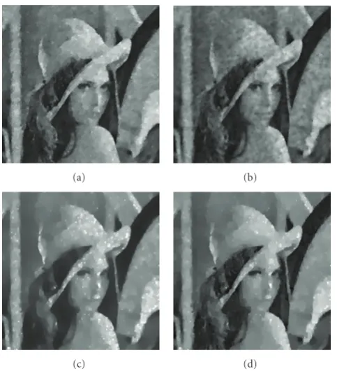
(c) (d)

Figure4: The restored “Lena” images for denoisingFigure 2(a): (a) by the proposed method (α1 =0.9×232,α2 =1.5×232, andζ =

5×10−3_{); (b) by the “HMW” method (α}

1=0.01,α2=0.004); (c)

by the “AA” method; (d) by the “RLO” method.

(a) (b)

(c) (d)

Figure5: The restored “Lena” images for denoisingFigure 2(b): (a) by the proposed method (α1 =0.5×232,α2 =0.2×232, andζ =

5×10−3_{); (b) by the “HMW” method (α}

1=0.01,α2 =0.01); (c)

by the “AA” method; (d) by the “RLO” method.

(a) (b)

(c) (d)

Figure 6: The restored “SynImag” images for denoising of

Figure 3(a): (a) by the proposed method (α1 = 4.6×232,α2 =

1.5×232_{, andζ =5×10}−3_{); (b) by the “HMW” method (α}

1 =

0.01,α2=0.01); (c) by the “AA” method; (d) by the “RLO” method.

(a) (b)

(c) (d)

Figure7: The restored SAR images for denoising ofFigure 3(b): (a) by the proposed method (α1 = 4×232,α2 = 18×232, andζ =

5×10−3_{); (b) by the “HMW” method (α}

1=0.01,α2=0.004); (c)

0 0.2 0.4 0.6 0.8 1 1.2 1.4

0 50 100 150 200 250 300

(a)

0.1 0.2 0.3 0.4 0.5 0.6 0.7 0.8 0.9

0 50 100 150 200 250 300

(b)

0.1 0.2 0.3 0.4 0.5 0.6 0.7 0.8 0.9

0 50 100 150 200 250 300

(c)

0.1 0.2 0.3 0.4 0.5 0.6 0.7 0.8 1 0.9

0 50 100 150 200 250 300

(d)

0.1 0.2 0.3 0.4 0.5 0.6 0.7 0.8 0.9

0 50 100 150 200 250 300

(e)

Figure8: The 60th line of the original, noisy, and restored images for denoisingFigure 2(a). (a) The noisy image; (b) the slice restored by the proposed method; (c) the slice restored by the “HMW” method; (d) the slice restored by the “AA” method; (e) the slice restored by the “RLO” method. Here the blue line is the original image, and the red line is the restored image.

The solution of the “HMW” model [21]

min

z,w ⎧ ⎨ ⎩

N2

i=1

[z]i+ [u0]ie−[z]i

+α1z−w2

2+α2TV(w)

⎫ ⎬ ⎭

(46)

is obtained by using the following alternating minimization algorithm:

z(m)=arg min

z N2

i=1

[z]i+ [u0]ie−[z]i

0 0.2 0.4 0.6 0.8 1 1.2 1.4 1.6

0 50 100 150 200 250 300

(a)

0 0.1 0.2 0.3 0.4 0.5 0.6 0.7 0.8 0.9

0 50 100 150 200 250 300

(b)

0 0.1 0.2 0.3 0.4 0.5 0.6 0.7 0.8 0.9

0 50 100 150 200 250 300

(c)

0 0.1 0.2 0.3 0.4 0.5 0.6 0.7 0.8 0.9

0 50 100 150 200 250 300

(d)

0 0.1 0.2 0.3 0.4 0.5 0.6 0.7 0.8 0.9

0 50 100 150 200 250 300

(e)

Figure9: The 100th line of the original, noisy, and restored images for denoisingFigure 2(b). (a) The noisy image; (b) the slice restored by the proposed method; (c) the slice restored by the “HMW” method; (d) the slice restored by the “AA” method; (e) the slice restored by the “RLO” method. Here the blue line is the original image, and the red line is the restored image.

w(m)_{=arg min}

w α1

z(m)_−w2

2+ TV(w)

. (48)

The corresponding nonlinear Euler-Lagrange equation of subproblem (47)

1−[u0]ie−[z]i+ 2α1

[z]i−

w(m−1)

i

=0,

i=1, 2,. . .,N2,

(49)

0 0.1 0.2 0.3 0.4 0.5 0.6 0.7 0.8 0.9

0 50 100 150 200 250 300

(a)

0 0.05 0.1 0.15 0.2 0.25 0.3 0.35 0.4

0 50 100 150 200 250 300

(b)

0 0.05 0.1 0.15 0.2 0.25 0.3 0.35 0.4

0 50 100 150 200 250 300

(c)

0 0.05 0.1 0.15 0.2 0.25 0.3 0.35 0.4

0 50 100 150 200 250 300

(d)

0 0.05 0.1 0.15 0.2 0.25 0.3 0.35 0.4

0 50 100 150 200 250 300

(e)

Figure10: The 128th line of the original, noisy, and restored images for denoisingFigure 3(a). (a) The noisy image; (b) the slice restored by the proposed method; (c) the slice restored by the “HMW” method; (d) the slice restored by the “AA” method; (e) the slice restored by the “RLO” method. Here the blue line is the original image, and the red line is the restored image.

The stopping criterion of the “HMW” method, the “AA” method, and the “RLO” method is that the PSNR value of the restored image reaches its maximum.

Our numerical experiments use several natural and manmade images such as “Lena” (Figure 1(a)), the synthetic

image (Figure 1(b)), and the SAR image (Figure 1(c)) to compare various algorithms’ performances. As shown in

Figure 2, the “Lena” images are corrupted by a Gamma noise withL = 33 (Figure 2(a)) and L = 5 (Figure 2(b)).

0 0.1 0.2 0.3 0.4 0.5 0.6 0.7 0.8 0.9

0 50 100 150 200 250

(a)

0 0.1 0.2 0.3 0.4 0.5 0.6 0.7 1

0.8 0.9

0 50 100 150 200 250

(b)

0 0.1 0.2 0.3 0.4 0.5 0.6 0.7 1

0.8 0.9

0 50 100 150 200 250

(c)

0 0.1 0.2 0.3 0.4 0.5 0.6 0.7 1

0.8 0.9

0 50 100 150 200 250

(d)

0 0.1 0.2 0.3 0.4 0.5 0.6 0.7 1

0.8 0.9

0 50 100 150 200 250

(e)

Figure11: The 128th line of the original, noisy, and restored images for denoisingFigure 3(b). (a) The noisy image; (b) the slice restored by the proposed method; (c) the slice restored by the “HMW” method; (d) the slice restored by the “AA” method; (e) the slice restored by the “RLO” method. Here the blue line is the original image, and the red line is the restored image.

corrupted by a Gamma noise withL =2, whileFigure 3(b)

shows the noisy SAR image which is distorted by Gamma noise withL=10.

Figures4,5,6, and7show the restored “Lena,” synthetic image and SAR images, respectively. In these experiments,

the initial guess is set to beu(0) _{= u0. It is clear that the}

Table1: The PSNR, ISNR, and ReErr of the restored images using four methods.

Experiments Our algorithm “HMW” algorithm “AA” algorithm “RLO” algorithm PSNR ISNR ReErr PSNR ISNR ReErr PSNR ISNR ReErr PSNR ISNR ReErr “Lena” inFigure 2(a) 27.973 7.914 0.0049 27.439 7.419 0.0056 27.016 6.950 0.0061 27.646 7.580 0.0053 “Lena” inFigure 2(b) 23.457 11.573 0.0139 21.032 9.131 0.0244 22.554 10.702 0.0171 23.143 11.291 0.0150 “SynImag” inFigure 3(a) 26.961 12.535 0.0279 22.338 7.860 0.0808 25.717 11.292 0.0371 25.841 11.416 0.0361 “SynImag” inFigure 3(b) 25.031 5.950 0.0252 24.579 5.589 0.0279 22.451 3.370 0.0456 22.657 3.5770 0.0435

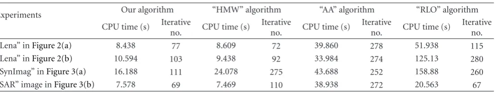
Table2: The number of iterations and computational times of four algorithms.

Experiments Our algorithm “HMW” algorithm “AA” algorithm “RLO” algorithm CPU time (s) Iterative

no. CPU time (s)

Iterative

no. CPU time (s)

Iterative

no. CPU time (s)

Iterative no.

“Lena” inFigure 2(a) 8.438 77 8.609 72 39.860 278 51.938 115

“Lena” inFigure 2(b) 10.594 103 9.438 92 33.984 274 125.13 280

“SynImag” inFigure 3(a) 16.188 111 24.078 275 43.688 252 158.88 260

“SAR” image inFigure 3(b) 7.578 69 7.469 110 38.938 272 20.563 67

proposed method is confirmed by the computing results of PSNR, ISNR, and ReErr of the three methods, as listed in

Table 1. FromTable 1, we can see that the PSNRs and ISNRs of the images restored by using our method are more than those restored by using the other three methods, and the relative errors ReErr are less than the other three methods. Moreover, our proposed algorithm is efficient.Table 2shows the number of iterations required for convergence and the computational times required by our method, the “HMW” method, the “AA” method, and the “RLO” method. Although our method takes little more time than the “HMW” method in some experiments, it is clear that the computational time required by our method is quite competitive with the other two methods.

We check the homogeneity of regions of interest in the image and analyze the loss (or the preservation) of contrast. In Figures 8, 9, 10, and 11, we show several lines of the original, noisy, and restored images. It is clear from the figures that the lines restored by the proposed method are better than those restored by the other three methods.Table 3

lists the results of mean square errors (MSEs) between the corresponding line of the original images and one of the restored images in Figures8–11. From the computing MSE results, we can conclude that our algorithm has the best performance.

We also prove that the proposed algorithm does not depend on starting point by experiment. In our experiment, we use two different initial guessed images in the proposed method. The first initial guess is set to be u(0) _{= u0, and}

the second is set to be a constant image where the constant is the mean ofu0. Here we do not give the restored images using the mean image as initial guess, because they are almost the same with those using the u(0) _{= u0. Table 4 shows}

that the PSNRs, ISNRs, and relative errors of the restored images using two different initial guesses are about the same. These means that our method is not sensitive to initial guess.

6. Conclusion

In this paper, we have investigated a new nonconvex varia-tional model for the multiplicative noise removal problem under the Weberized TV regularization framework. Using a reference energy functional, we propose another surrogate strictly convex objective function for multiplicative noise removal. Our algorithm is designed using the well-known variable-splitting and penalty techniques in optimization. The proposed algorithm contains three subminimizing parts and each of them permits a closed-form solution. Our experimental results show that our proposed algorithm is effective and efficient to filter out multiplicative noise while well preserving the significant details.

Appendix

Proof of

Theorem 1

Let us denote thatα = infΩ(u0),β = supΩ(u0), TV(u) =

Ω|∇u|dx,Edata(u) =

Ω(u−u0logu)dx, andh(s) = s− u0logs. It is obvious that h(s) = u0/s2 _{andh is strictly}

convex asu0 > 0. Therefore, we haveh(s)≥ u0−u0logu0

for alls∈R2_{. This implies thatE}

R(u) has a lower bound for

allu ∈ BV(Ω). Hence we consider a minimizing sequence

{un} ∈BV(Ω) for (16).

First, we show thatα ≤ un ≤ β. Sinceu0 ∈ L∞(Ω) is

a positive, bounded function with infΩu0 > 0, we choose a

sequence{un} ∈ C∞(Ω) such that un → u0 inL1(Ω) and

a.e. inΩ asn → ∞, and infΩ(u0) ≤ un ≤ supΩ(u0). We

remark thath(s) is decreasing ass∈(−∞,u0) and increasing as s ∈ (u0, +∞). Therefore, if M > u0, one always has

h(min(s,M)) ≤ h(s). Hence, if we let M = β = sup(u0), then

Table3: The mean square error between the line of the original images and the restored images using four algorithms.

Experiments Our algorithm “HMW” algorithm “AA” algorithm “RLO” algorithm

“Lena” inFigure 2(a) 0.4892 0.5134 0.5512 0.5034

“Lena” inFigure 2(b) 0.8905 1.2748 1.0664 1.0778

“SynImag” inFigure 3(a) 0.4147 0.5309 0.5502 0.5355

“SAR” image inFigure 3(b) 1.0903 1.1204 1.1729 1.1294

Table4: The PSNR, ISNR, and ReErr of the restored images using two different initial guesses in our algorithms.

Experiments u(0)=u0 u(0)=mean(u0)

PSNR ISNR ReErr PSNR ISNR ReErr

“Lena” inFigure 2(a) 27.973 7.914 0.0049 28.001 7.981 0.0049

“Lena” inFigure 2(b) 23.457 11.573 0.0139 23.564 11.663 0.0136

“SynImag” inFigure 3(a) 26.961 12.535 0.0279 27.003 12.524 0.0276

“SAR” image inFigure 3(b) 25.031 5.950 0.0252 25.003 6.013 0.0253

Moreover, we have that (e.g., see [37, Section 4.3, Lemma 1]):

TVinfu,β≤TV(u). (A.2) Combining (A.1) and (A.2), we thus deduce that

ER

infu,β≤ER(u). (A.3)

And we get in the same way that

ER

sup(u,α)≤ER(u). (A.4)

Therefore, we can assume without restriction that infΩ(u0)≤ un≤supΩ(u0).

Second, the above proof implies in particular thatunis

bounded inL1_{(Ω). Moreover, by the definition of{u}

n}, we

get that there exists a constantCsuch that

TV(un) +λEdata(un)≤C. (A.5)

Moreover, standard computations show that Edata(un)

reaches its minimum value whenu=u0and thus we deduce that TV(un)≤C.

Therefore, we get thatunis bounded in BV(Ω) and there

existsu∈BV(Ω) such that up to a subsequence,un → uin

BV(Ω)-weak∗andun → uinL1(Ω)-strong. Necessarily, we

have 0≤α≤u≤β, and thanks to the lower semicontinuity of the total variation and Fatou’s lemma, we get thatuis a solution of problem (16).

Sinceh is strictly convex asu0 > 0, the uniqueness of the minimizer follows from the strict convexity of the energy functional in (16). This completes the proof.

Acknowledgments

The authors would like to express their gratitude to the anonymous referees for making helpful and constructive suggestions, especially for the proof of the algorithm’s convergence. This work is supported in part by the Natural Science Foundation of China under Grant no. 60802039 and 60672074 and by the National 863 High Technology Development Project under Grant no. 2007AA12Z142.

References

[1] G. Steidl and T. Teuber, “Removing multiplicative noise by Douglas-rachford splitting methods,”Journal of Mathematical Imaging and Vision, vol. 36, no. 2, pp. 168–184, 2010. [2] T. Chan and J. Shen,Image Processing and Analysis-Variational,

PDE, Wavelet, and Stochastic Methods, SIAM, Philadelphia, Pa, USA, 2005.

[3] G. Aubert and P. Kornprobst,Mathematical Problems in Image Processing, vol. 147 ofApplied Mathematical Sciences, Springer, London, UK, 2002.

[4] M. A. T. Figueiredo and R. D. Nowak, “An EM algorithm for wavelet-based image restoration,”IEEE Transactions on Image Processing, vol. 12, no. 8, pp. 906–916, 2003.

[5] J. M. Bioucas-Dias, “Bayesian wavelet-based image deconvo-lution: a GEM algorithm exploiting a class of heavy-tailed priors,”IEEE Transactions on Image Processing, vol. 15, no. 4, pp. 937–951, 2006.

[6] J. Ma and G. Plonka, “Combined curvelet shrinkage and nonlinear anisotropic diffusion,”IEEE Transactions on Image Processing, vol. 16, no. 9, pp. 2198–2206, 2007.

[7] L. I. Rudin, S. Osher, and E. Fatemi, “Nonlinear total variation based noise removal algorithms,”Physica D, vol. 60, no. 1–4, pp. 259–268, 1992.

[8] J. P. Oliveira, J. M. Bioucas-Dias, and M. A. T. Figueiredo, “Adaptive total variation image deblurring: a majorization-minimization approach,”Signal Processing, vol. 89, no. 9, pp. 1683–1693, 2009.

[9] A. Buades, B. Coll, and J. M. Morel, “A review of image denoising algorithms, with a new one,” SIAM Journal on Multiscale Modeling and Simulation, vol. 4, no. 2, pp. 490–530, 2005.

[10] L. Alvarez, F. Guichard, P.-L. Lions, and J.-M. Morel, “Axioms and fundermental equations of image processing,”Archive for Rational Mechanics and Analysis, vol. 16, no. 9, pp. 200–257, 1993.

[11] W.-Z. Shao and Z.-H. Wei, “Edge-and-corner preserving regularization for image interpolation and reconstruction,” Image and Vision Computing, vol. 26, no. 12, pp. 1591–1606, 2008.

[13] J. S. Lee, “Digital enhancement and noise filtering by use of local statistics,”IEEE Transactions on Pattern Analysis and Machine Intelligence, vol. 2, no. 2, pp. 165–168, 1980. [14] D. T. Kuan, A. A. Sawchuk, T. C. Strand, et al., “Adaptive noise

smoothing filter for images with signal dependent noise,”IEEE Transactions on Pattern Analysis and Machine Intelligence, vol. 7, no. 2, pp. 165–177, 1985.

[15] Y. Yu and S. T. Acton, “Speckle reducing anisotropic diffusion,” IEEE Transactions on Image Processing, vol. 11, no. 11, pp. 1260–1270, 2002.

[16] K. Krissian, C.-F. Westin, R. Kikinis, and K. G. Vosburgh, “Oriented speckle reducing anisotropic diffusion,”IEEE Trans-actions on Image Processing, vol. 16, no. 5, pp. 1412–1424, 2007. [17] G. J. Liu, X. P. Zeng, F. C. Tian, Z. Z. Li, and K. Chaibou, “Speckle reduction by adaptive window anisotropic diffusion,” Signal Processing, vol. 89, no. 11, pp. 2233–2243, 2009. [18] L. I. Rudin, P. L. Lions, and S. Osher, “Multiplicative denoising

and deblurring: theory and algorithms,” inGeometric Level Set Methods in Imaging, Vision, and Graphics, S. Osher and N. Paragios, Eds., pp. 103–120, 2003.

[19] G. Aubert and J. F. Aujol, “A variational approach to remove multiplicative noise,”SIAM Journal on Applied Mathematics, vol. 68, no. 4, pp. 925–946, 2008.

[20] J. Shi and S. Osher, “A nonlinear inverse scale space method for a convex multiplicative noise model,”SIAM Journal on Applied Mathematics, vol. 1, no. 3, pp. 294–321, 2008.

[21] Y. M. Huang, M. K. Ng, and Y. M. Wen, “New total variation method for multiplicative noise removal,”SIAM Journal on Imaging Sciences, vol. 2, no. 1, pp. 22–40, 2009.

[22] S. Durand, J. Fadili, and M. Nikolova, “Multiplicative noise cleaning via a variational method involving curvelet coeffi -cients,” in Scale Space and Variational Methods, A. Lie, M. Lysaker, K. Morken, and X.-C. Tai, Eds., Springer, Voss, Norway, 2009.

[23] J. H. Shen, “On the foundations of vision modeling: I. Weber’s law and Weberized TV restoration,”Physica D, vol. 175, no. 3-4, pp. 241–251, 2003.

[24] J. H. Shen and Y.-M. Jung, “Weberized Mumford-Shah model with Bose-Einstein photon noise. ,”Applied Mathematics and Optimization, vol. 53, no. 3, pp. 331–358, 2006.

[25] Z. H. Wei, Y. Q. Fu, Z. G. Gao, and S. X. Cheng, “Visual compander in wavelet-based image coding,”IEEE Transactions on Consumer Electronics, vol. 44, no. 4, pp. 1261–1266, 1998. [26] Z. H. Wei, P. Qin, Y. Q. Fu, and S. X. Cheng, “Perceptual

digital watermark of images using wavelet transform,”IEEE Transactions on Consumer Electronics, vol. 44, no. 4, pp. 1267– 1272, 1998.

[27] E. H. Weber, “De pulsu, resorptione, audita et tactu,” in Annotationes Anatomicae et Physiologicae, Koehler, Leipzig, Germany, 1834.

[28] L. C. Evans and R. F. Gariepy, Measure Thoery and Fine Properties of Functions, CRC Press, Boca Raton, Fla, USA, 1992.

[29] A. Chambolle, “An algorithm for total variation minimization and applications,”Journal of Mathematical Imaging and Vision, vol. 20, no. 1-2, pp. 89–97, 2004.

[30] T. F. Chan, G. H. Golub, and P. Mulet, “A nonlinear primal-dual method for total variation-based image restoration,” SIAM Journal of Scientific Computing, vol. 20, no. 6, pp. 1964– 1977, 1999.

[31] T. F. Chan and P. Mulet, “On the convergence of the lagged diffusivity fixed point method in total variation image restoration,”SIAM Journal on Numerical Analysis, vol. 36, no. 2, pp. 354–367, 1999.

[32] T. F. Chan and J. H. Shen,Theory and computation of varia-tional image deblurring, Lecture Notes Series, IMS, Singapore, 2006.

[33] T. F. Chan, J. H. Shen, and L. Vese, “Variational PDE models in image processing,”Notices of the American Mathematical Society, vol. 50, pp. 14–26, 2003.

[34] Y. Wang, J. Yang, W. Yin, and Y. Zhang, “A new alternating minimization algorithm for total variation image reconstruc-tion,”SIAM Journal on Imaging Sciences, vol. 1, no. 3, pp. 248– 272, 2008.

[35] Y. Wang, J. Yang, W. Yin, and Y. Zhang, “A fast algorithm for image deblurring with total variation regularization,” Tech. Rep. TR07-10, Rice University CAAM, Houston, Tex, USA. [36] J. Nocedal and S. J. Wright,Numerical Optimization, Springer,

Berlin, Germany, 2000.