Thermalization in Periodically-Driven Interacting Quantum Systems

(1)

Systems

Thesis by

Karthik Iyengar Seetharam

In Partial Fulfillment of the Requirements for the Degree of

Doctor of Philosophy

CALIFORNIA INSTITUTE OF TECHNOLOGY Pasadena, California

2018

(2)

Karthik Iyengar Seetharam ORCID: 0000-0003-1928-8019

(3)

ACKNOWLEDGEMENTS

My life has been filled with joy, comfort, adventure, and incredible intellectual growth due to the endless and unwavering support of my loving family, friends, advisor, and delightful collaborators without whom I would not be writing this thesis today. Few words can describe my debt and gratitude. My obeisance to you all.

1

(4)

ABSTRACT

Periodically-driven (Floquet) quantum systems are ubiquitous in science and technology. For example, when a laser illuminates a material or an AC voltage is applied to a device, the system is well-described by a time-periodic Hamiltonian. In recent years, periodic driving has been proposed, not just as a tool to excite and probe devices, but actually as a mechanism ofengineeringnew phases of matter, some of which have no equilibrium analog. However, with this promise comes a serious problem. Intuitively, if energy is injected into and distributed throughout a system, it is no surprise that it tends to heat up indefinitely to infinite temperature.

(5)

PUBLISHED CONTENT AND CONTRIBUTIONS

[1] Karthik Seetharam, Paraj Titum, Michael Kolodrubetz, and Gil Refael. Absence of thermal-ization in finite isolated interacting floquet systems. Phys. Rev. B, 97:014311, Jan 2018. doi: 10.1103/PhysRevB.97.014311. URL https://link.aps.org/doi/10.1103/PhysRevB. 97.014311.

K.I.S. participated in the conception of the project, performed numerical simulations, made primary contributions to the results, and participated in the writing of the manuscript.

[2] Karthik I. Seetharam, Charles-Edouard Bardyn, Netanel H. Lindner, Mark S. Rudner, and Gil Refael. Controlled population of floquet-bloch states via coupling to bose and fermi baths. Phys. Rev. X, 5:041050, Dec 2015. doi: 10.1103/PhysRevX.5.041050. URL https: //link.aps.org/doi/10.1103/PhysRevX.5.041050.

K.I.S. performed calculations and numerical simulations, made primary contributions to the results, and participated in the writing of the manuscript.

(6)

LIST OF ILLUSTRATIONS

Number Page

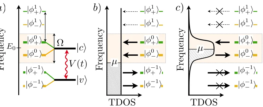
2.1 Carrier kinetics in a Floquet-Bloch system coupled to Bose and Fermi reservoirs. a) One dimensional semiconductor wire coupled to an energy-filtered fermionic reservoir. Energy filtering is achieved by coupling the system and reservoir via a deep impurity band in a large bandgap semiconductor. b) Band structure of the non-driven system. The driving field photon energy~Ωexceeds the bandgapEgap, causing

resonant coupling at crystal momentum values ±kR. c) Floquet band structure, indicating the character of the Floquet band in terms of the original conduction (blue) and valence (red) bands. Coupling to acoustic phonons mediates electronic momentum and energy relaxation (orange arrows), while radiative recombination scatters electrons vertically between conduction and valence band like states (purple arrow). At half filling, the steady state resembles that of an insulator with a small density of excited electrons and holes. . . 52 2.2 Harmonic structure of Floquet states and energy-filtered reservoir coupling. a)

Floquet harmonics of a two-level system with states |vi and |cicoupled by an on-resonancedriving fieldV(t). The Floquet zone (shaded) is centered at the energyE0,

set equal to the energy of the resonant state|ci. In the special case of a rotating-field,

V(t) = 1

2V0e

−iΩt_|

cihv|+h.c., we have|φ0_±i= |ci, |φ−_±1i= ±|viandE± = E0± 1₂V0,

see Eq. (2.3). Away from resonance, the relative normalizations of |φn₊i and |φn₋i will change. For a more general form of weak driving, the dominant harmonics are shown in bold. b) The Floquet states |ψ±(t)i are both coupled to filled and empty states of a wide-band reservoir via the harmonics {|φn_±i}, see Eq. (2.10). Here the reservoir chemical potential is set in the gap of the non-driven system. c) When coupling is mediated by a narrow-band energy filter, the tunneling density of states (TDOS) and photon-assisted tunneling are suppressed outside the filter window. By setting the reservoir chemical potential inside the Floquet gap, centered around the energy E0in the original conduction band (see Fig. 2.1b), the lower and upper

(9)

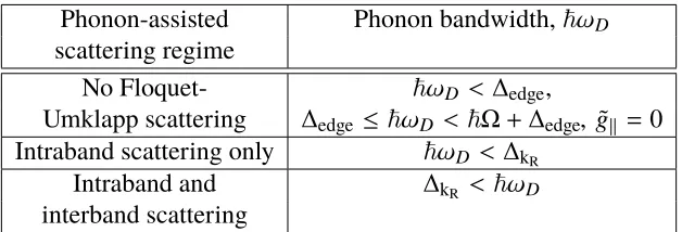
2.3 Numerically obtained steady states with radiative recombination and coupling to acoustic phonons. Here the density is set to half-filling, and we use a 3D acoustic phonon bath with ~ωD smaller than the gap ∆edge at the Floquet zone edge. The

phonon temperature is set to kBT = 10−2~Ω. We keep the phonon and photon densities of states fixed, and only vary an overall scale for the coupling matrix elements. The full details of the model can be found in Table 2.2. (a) Distribution of electrons in the upper Floquet band, Fk+ = hf_k†₊fk+i, for several values of κ =

kRW

rec

/πΛinter_{, see Eq. (2.9) and Appendix 2.C for definitions. The distributions}

are fitted to a Floquet-Fermi-Dirac distribution at temperatureT(solid lines). Due to particle-hole symmetry, the distributions of holes in the lower Floquet band, 1−Fk−, are identical to the distributions shown. Inset: Log-Log plot showing the total density of electrons in the upper Floquet band, ne as a function of κ. The density

ne is normalized to the “thermal density” nth = 6.8×10−4 (see text). The plot

(10)

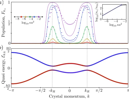
2.4 Numerically obtained steady states of the system coupled to both bosonic and fermionic baths. The top and bottom panels show the distributions of electrons in the Floquet + and - bands, respectively, for increasing strength of the coupling to the Fermi reservoir. We characterize the coupling strength by the ratio of tunneling and recombination rates,Υ= 2Γ0_k

R,+/W

rec

(see Eqs. (2.8) and (2.10) for definitions of the rates). Two types of Fermi reservoirs are studied. (a) Wide-band Fermi reservoir, whose Fermi level lies in the middle of the original bandgap (the bandgap ofH0). An increase in the coupling strength to such a reservoir leads to a substantial

increase in the electron and hole densities ne and nh, due to photon assisted tun-neling. (b)Energy filtered Fermi reservoir, whose Fermi level lies at the resonance energyE0 in the original conduction band, i.e., in the middle of the Floquet gap of

(11)

2.5 Electron and holes densities ne and nh in the steady state of the system coupled to bosonic baths (acoustic phonons and recombination) and anenergy filteredfermionic reservoir. The figure clearly demonstrates that (1) the steady state densitiesne and

nh are insensitive to small shifts of the reservoir’s chemical potential µres near the

middle of the Floquet gap, and (2) a sufficiently strong coupling to the reservoir can effectively suppress the electron and hole densities when µres is within the Floquet

gap. Panel (a) shows the total density ¯n=ne+nhas a function of the Fermi level of the reservoir µres and the coupling strength ratioΥ= 2Γ_k0_R_,₊/W

rec

. As long as µres

is within the Floquet gap,neandnhremain low. Onceµres enters the Floquet+or−

bands, the system becomes metallic and the electron (hole) densityne(nh) is set by the Fermi level of the reservoir. This behavior is seen in in panel (b), where we plot

ne. To further demonstrate the incompressible regime, in (c) we show ¯nas a function of µres for several coupling strengths to the reservoir, corresponding to the dotted

lines in panel (a). Panel (d) gives the the electron and hole densities, ne (circles) and nh (squares) for two values of µres: in the middle of the Floquet gap (black)

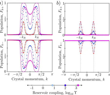
and at the edge of the + Floquet band (red). In the first case, the results explicitly demonstrate the suppression of the excitation densities ne and nh with increasing reservoir coupling. Model parameters are the same as in Fig. 2.4. . . 75 2.D.1 Scattering rates (red), Rα(k), [see Eq. (2.50)] in the steady state of the system. The

top (bottom) plot corresponds to the upper (lower) Floquet band. Also shown (blue) are the distributionsne(k)annh(k)in each Floquet band. In panel (a), we show the case of half-filling, with no reservoir coupling (corresponding to Fig. 2.3 in the main text) while in (b) we take log₁₀(Υ)=3.15. Other model parameters are the same as for the green (middle) curve in Fig. 2.3. Note the enhanced scale for the rates in the bottom plots, and the enhanced scale for the distributions in panel (b). . . 96 2.E.1 The offset density ∆n. Panel (a) shows ∆n as a function of the reservoir chemical

potential µres, and the coupling of the Fermi reservoir log10Υ. Incompressible

behavior can be seen when µres ≈ 0. (b) Vertical cuts of panel (a), showing∆nas

a function of µres for several coupling strengths to the Fermi reservoir, with values

(12)

3.1 Quasienergy band structure and interband scattering processes. Electron-electron interactions yield three different types of interband processes: Auger, and Floquet-Auger (FA) of types I and II (see text) depicted by dashed, dotted, and solid lines, respectively. In the Floquet-Auger processes, the sums of quasienergies of the electrons in the initial and final states differ by an integer multiple of the driving frequency, ~Ω. Interband scattering resulting from electron-phonon interactions yields two important processes: (i) relaxation from the upper to the lower band via phonon emission, and (ii) excitation from the lower to the upper band. This process can occur even at zero temperature, as a Floquet-Umklapp (FU) process, which involves phonon emission and absorption of~Ωfrom the driving field. . . 106 3.1 Left: Steady-state populations in the UF band,Fk+, for several values of the effective

cooling strengthG2₀/V₀2. Results are obtained from the FBE, Eqs. (3.5) and (3.9), with phonon bandwidth ΩD/∆A = 2.2 and phonon temperatureTph = ∆A/10. Dashed lines indicate the crystal momentum values where the UF band minima are located. For low values of G2₀/V₀2, the steady state is “hot,” with nearly uniform occupation

Fk+ ≈0.5 for allk. For large values ofG2₀/V₀2, the steady state is “cold”, and features a low density of excitations concentrated around the minima of the UF band. Solid lines show fits to a Floquet-Fermi-Dirac distribution with effective chemical potential

µ∗

+ (with respect to E = 0), and temperatureT∗, taken as free parameters. Right:

extracted values ofµ∗₊andT∗vs. G₀2/V₀2. Whenµ∗₊ _,0, the steady state is described by a “double” Floquet-Fermi-Dirac distribution, with separate chemical potentials for electrons and holes in the UF and LF bands, respectively. The gray shaded region in upper panel denotes a regime where the fits are sensitive only to the value ofT∗

(13)

3.1 Left: Excitation densityn= n₊, Eq. (3.6), as a function of the (normalized) phonon bandwidthΩD/∆A andG2₀/V₀2. For largeG2₀/V₀2, the phonon bath effectively cools the system, and the steady-state excitation density is low (blue color). The cutoff

(14)

3.A.1 Dominant types of scattering processes leading to single-particle excitations across the Floquet gap, classified according to their origin: phonon relaxation and electron-electron interactions — Auger I, Floquet-Auger I, and Floquet-Auger II, as in the main text. Recall that Floquet-Auger processes of type I (II) create one (two) excitation(s) across the Floquet gap. The energy bands shown here are copies of the bands of the non-driven system (dark blue) shifted bymΩ, i.e., by integer multiples of the drive frequency. Bands are labeled by m, and shown in different colors for distinctm. They can be regarded as the Floquet modes (harmonics) composing the Floquet states of the system, in the limit of a small drive amplitude S Ω. Here we choose our basis of Floquet states so that the latter have dominant Floquet-mode components in the Floquet zone (energy windowΩ) highlighted in grey. Scattering processes can be decomposed into transitions between Floquet modes (initial/final states denoted by red/green dots), and we only illustrate the dominant ones involving leading-order Floquet-mode components. Transitions between Floquet states must conserve momentum and energy, up to an integer multiple nΩ (and up to some phonon momentum and energy, for phonon-mediated processes). Normal processes are characterized byn= 0 (black arrows) and Floquet-Umklapp (FU) processes are characterized byn_,0 (red and orange arrows). The dotted lines indicate the virtual transitions involved in a process, with each virtual transition involving an additional power of S/Ω. The suppression factors of individual processes are indicated below each panel. When the lower Floquet band is filled, Auger I and Floquet-Auger I processes are absent. Note that the “B” phonon relaxation process can beO(1)if the phonon matrix elements Gν_νk0k0(q)allow interband (off-diagonal inν, ν0) transitions. This scenario exists, for example, in the case of radiative recombination. . . 124 4.1 Phase diagram showing the thermal (red) and non-thermal (blue) behavior of the

(15)

4.1 Quasienergy spectrum for N = 10 (a) and N = 12 (b) at Ω/J = 0.83. Blue dots denote strong interactionU/J = 100 and red dots denote weak interactions at

U/J = 0.59. We see that weak interactions give rise to a continuous spectrum. In contrast, the strong interactions yield separation of the spectrum into quasienergy plateaus reflecting the influence of doublons (Í

inini+1). Increasing system size

softens the plateaus. . . 138 4.2 Time evolution of three initial states for weak and strong interactions (U/J = 0.59

and U/J = 100 respectively): A = |101010...i, B = |111...000i, and C =

(C_N/N 2)

−1/2ÍC N N/2

i=1 |ii. For weak interactions all states thermalize as expected. For

strong interactions, the initial states with non-thermal doublon values (A,B) maintain non-thermal values over time whereasC remains thermal. . . 139 4.1 Histogram of Dn measured in each Floquet eigenstate as a function of U/J and

system size. ForU/J 1, the spectrum displays some spread in the doublon density due to near-integrability close to the free fermion limit U = 0. At U/J ∼ O(1), however, sufficient mixing leads to a tight squeeze of D around 0.5, indicating a thermal region. At strong interactions U/J 1, there is significant spread of D

also indicating non-thermal behavior. . . 141 4.2 Dependence of doublon log spectral variance on coupling and and system size.

Fig-ure a) shows raw data which demonstrate the three regions clearly, near-integrability for J/U 1, thermal for J/U ∼ O(1), and non-thermal (also near-integrability) for J/U 1. The black stars indicate the approximate midpoint of the crossover region. Figure b) rescales the axes to show the scaling collapse of the thermal region indicating simple exponential behavior independent of coupling. Figure c) rescales the axes differently to show the scaling collapse of the non-thermal region with

(16)

4.1 Dependence of the doublon log spectral variance on coupling and system size for both HF and H

[2]

F . Figure a) compares the data from Figure 4.2c to the same data gathered from H_F[2]. Note that H_F[2] has a different scaling form as shown in the inset, displaying a much weaker dependence on system size. Breakdown of the HFE happens faster than the breakdown of integrability within the HFE, apparently resulting in a direct transition from integrability to an infinite temperature Floquet-ETH phase. Figure c) depicts this scenario in the bold top box while displaying an alternative possibility in the bottom box which contains an intermediate finite-temperature ETH phase. Figure b) displays the average log participation ratio (LPR) of exact Floquet eigenstates in the basis of zeroth-order HFE eigenstates. Note that the LPR has the same scaling form as the log spectral variance and is a good measure of delocalization (here due to resonances) of exact Floquet eigenstates in the basis of zeroth-order HFE states. An explicit example of this is shown in the inset for a representative exact Floquet eigenstate. . . 147 4.A.1 Frequency dependence of spectral doublon variance as a function of couplingU/J

at N = 12. Figure a) shows frequency along the y-axis and coupling along the x-axis with color denoting the variance value. Figure b) shows cuts at particular frequencies. In the high frequency limit, the system is approximated by the time-averaged lab frame Hamiltonian, leading to a variance given by static free fermions. In the low-frequency limit, we get the variance behavior discussed in the text which shows the thermal to non-thermal transition as U/J gets larger. At intermediate frequencies, the rare resonances govern the precise details of the variance (e.g. peaking) and the system is quite sensitive to drive parameters. . . 152 4.B.1 Waveform dependence of spectral doublon variance as a function of couplingU/Jat

Ω/J = 0.83. A square wave is given byn=2 and a cosine is closely approximated by n = 100. In between, the discretization of sampling a waveform gives rise to dampening and resurgence effects as can be understood by considering the time-evolution operator over one periodU(T,0)(see text). Overall, the thermal to non-thermal transition persists for a cosine drive but has significantly slower crossover behavior as compared to the square drive. . . 153 4.C.1 Harmonic coefficients of ei xF(Ωt) in Eqn. 4.15 for the square wave which control

(17)

4.C.2 Quasienergies of the exact HF and the effective Hamiltonians ˜H0andH

[2]

F for three values of U/J. At largeU/J, the spectra match, while away from this limit it is clear that H_F[2] is a good approximation over some region before the breakdown of the high frequency expansion. . . 159 4.D.1 Level statistics of the exact HF and the effective Hamiltonian H

[2]

F . For the static HamiltonianH_F[2], only the middle 50% of the spectrum is used to avoid noise from the often-anomalous high and low energy tails. For small U/J, the level statistic is GOE indicating non-integrable behavior of the system. As U/J increases, the level statistic breaks away from GOE indicating a different spectral structure due to near-integrability. Note that this crossover is system size dependent as seen clearly in a). In b), there is a much weaker system size dependence suggesting that the HFE, at second order, does not accurately capture the crossover from integrability to non-integrability. . . 160 4.D.2 Expectation values of the doublon densityDand effective HFE Floquet Hamiltonian

H_F[2] ≡ e−iKeff[2](0)H[2]

effe

iK_eff[2](0)

in exact Floquet eigenstates ofHF. . . 161 4.D.3 Frobenius norm of the integrable model ˜H0and of the second order termH

[2]

eff in the

HFE normalized to the trace norm of the identity for each system size. As discussed in Appendix 4.C, the trace norm has(J/U)2behavior indicated by the dashed line. At J/U ∼ 0.5, the second order term is relatively larger than the integrable part. Both zeroth order and second order terms have the same system size dependence as seen by observing the relative trace norm in the inset. This fact immediately rules out the possibility of that the breakdown of the HFE as an operator expansion is responsible for thermalization as discussed in section 4.5 and appendix 4.D, at least at second order. . . 162 6.1 Steady-state occupation of the lower Floquet band as a function of the ratio of

bare electronic interaction (V) and electron-phonon (G) couplings (scaled by ρ, the partial density of states for the phonon bath). As interactions get stronger relative to the phonons (which cool the system), the system heats up from a near perfect Floquet-insulator state to the an almost infinite temperature state. . . 205 6.2 Steady-state magnitude of the off-diagonal Floquet-band polarization. We see that

(18)

LIST OF TABLES

Number Page

2.1 Summary of the different regimes of scattering processes assisted by acoustic phonons. Interband and Floquet-Umklapp processes are active or inactive depending on the relation between the phonon bandwidth ~ωD and the relevant Floquet gap:

∆kR is the Floquet gap atE = 0, while∆edge is the Floquet gap at the Floquet zone edge,E = ~Ω/2. The drive parameter ˜gk is defined through Eq. (2.2). . . 63 2.2 Parameters fixed in all simulations. Top row: parameters of the electronic

Hamilto-nian, Eq. (2.1), with Ek = 2A[1−cos(ka)]+ Egap, where ais the lattice constant.

The drive is spatially uniform,V(t) = 1

2V0(g· σ)cosΩt. Bottom row: parameters

of the three dimensional acoustic phonon bath, where cs is the phonon velocity, and ωD is the Debye frequency. In all simulations, the overall scale of the phonon matrix elements is set by fixing the ratio 2π(G₀ph)2_ρ_¯ph_/(_~_Ω₎_{, where ¯}_ρph_{is the phonon}

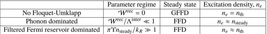
density of states at zero momentum and energy ~cs(π/a). For convergence, in the simulations we keep the phonon bath at a small temperature, kBT ≈ 10−2~Ω. . . 66 2.3 Summary of main results for the steady state distributions in different regimes.

FFD denotes a steady state in which electrons and holes in Floquet bands + and − are described by separate Fermi-Dirac distributions with independent chemical potentials (at the bath temperature). GFFD stands for a global Floquet-Fermi-Dirac distribution, with a single chemical potential. Other symbols: nth stands for the

thermal excitation density, while nsteady is defined in Eq. (2.9). The parameter Υ

characterizing the tunneling rate to the Fermi reservoir is defined in Eq. (2.13), and Wrec _and_Λinter _{characterizing recombination and phonon mediated interband}

(19)

C h a p t e r 1

INTRODUCTION

1.1 General Introduction

With recent advances in fabrication, cooling, and laser technologies, quantum physics is now at the forefront of modern science and engineering. In particular, nonequilibrium physics is a challenging frontier rife with opportunity from both a scientific and a technological perspective. Not only are universal predictions and precise quantitative statements scarce, but even the qualitative dynamical behavior of many-body systems, classical or quantum, are not fully understood. Only with a solid understanding can we hope to control quantum many-body systems. The necessity of understanding quantum dynamics is clearly exemplified by the rudimentary tasks encountered in building and operating a quantum computer. To have a fully functional device, one must be able to, with high fidelity, prepare many-qubit states of interest, execute single and two-qubit gate operations, and perform controlled measurements to observe an output, all while being robust to environmental noise. In any platform of interest (e.g. trapped ions or transmon qubits), “doing” any of these steps means altering the physical system in real-time, i.e. a dynamical or nonequilibrium process. While current efforts to build a quantum computer have shown significant progress, a thorough understanding of many-body dynamics and subsequent methods to control them is essential to usher in an age of quantum technology.

One corner of the nonequilibrium landscape is periodically-driven (Floquet) quantum systems and is the topic of this thesis. Floquet systems naturally arise in a variety of experimental platforms. For example, when a laser drives a system or when an oscillatory electrical voltage is applied to a device, the system is well-described by a time-periodic Hamiltonian. Hence, practical tools used to control, excite, and understand real devices many times fall under the broad umbrella of Floquet systems.

In recent years, periodic driving has been proposed, not just as a tool to excite and probe devices, but actually as a mechanism forengineeringnew phases of matter. These Floquet systems can not only exhibit unique phases of matter that do not exist in equilibrium, but also by construction carry the possibility of engineering states of matter in a controlled way, particularly when combined with dissipation and novel device architectures. In fact, the recent adoption of the name Floquet engineering aptly describes much of the research efforts in using periodic driving to induce and control dynamical behavior.

(20)

bands of a simple 2d semiconductor in such as a way as to obtain a nonequilibrium topological phase hosting edge states. This is known as the “Floquet Topological Insulator” (FTI) in analogy to its equilibrium counterpart. This major breakthrough stimulated and intense push to study the extent to which periodic driving could induce new phases of matter. Through this effort emerged the so-called “anomalous” Floquet phases, or rather, periodically-driven phases of matter that do not have any equilibrium counterpart. Examples of these include a quantum hall effect with no delocalized bulk modes known as the “Anomalous Floquet Anderson Insulator” [82] and the “time-crystal” [20, 90] which is a system that spontaneously breaks the periodic time translation symmetry and hosts subharmonic responses. Theoreticians have gone to great lengths to classify all the types of topological phases that exist when augmenting a system with periodic driving though concrete models and experimental proposals are a subject of ongoing work [19, 20, 28, 39, 58, 59, 63– 65, 70–72, 82, 85, 86, 90].

Experimental realizations of Floquet phases are also intensely being pursued. Gedik et al. [87] illuminated the surface of a TI with laser light and showed that Floquet bands can be observed via time-resolved angle-resolved-photoemission- spectroscopy (ARPES), at least transiently. Rechts-man et al. [67] have demonstrated an analog of the FTI in photonic crystals where wave propagation is described by the paraxial Schrodinger equation. Periodic driving has also been used to induce artificial gauge fields in cold atomic systems thus providing another avenue for engineering more complex Hamiltonians useful for studying under analog quantum simulation [11, 26]. Aidelsberger et al. [4] and Miyake et al. [54] have both used this to realize the Harper-Hofstader model, and Jotzu et. al [36] have used this technique to realize the Haldane model, all in ultracold atomic gases. Time crystals have been experimentally demonstrated in diamond nitrogen vacancy (NV) centers in Choi et al. [10] and in interacting spin chain of trapped ions in Zhang et al. [92]. Finally, Parker et al. [57] utilize periodic shaking to generate spin interactions strong enough to create ferromagnetic domains.

While the intense activity in Floquet physics is warranted and exciting, there is one major im-pediment blocking the immediate success of Floquet engineering. If one periodically shakes or (laser) blasts a systemresonantlythereby inputting energy, and allows that energy to be distributed throughout the system (e.g. through interactions), would the system not just heat up indefinitely? If every Floquet system just kept heating up, there would be no hope in observing new physics or having any means of control. Clearly this is an undesirable end and so one must study when this intuition is in fact true, and if so, how to avoid it. This problem of heating is what prevents a generic resonant Floquet system from becoming useful.

(21)

appropriately such that the nonequilibrium steady state (NESS) of system is controlled. This is the subject of chapters 2 and 3 and Refs. [14, 31, 32, 76].Second, one can still isolate the system but hope to find parameter regimes in which the heating process is slow compared to any desired physics of interest. This is called prethermalization, or rather finding regimes where there are long-lived transient states [2, 9, 21, 44, 52, 88, 91]. A “dual” version of prethermalization is to look for stationary states of finite systems that do not exhibit maximal entropy (heating). This is the subject of chapter 4. Third, one can study integrable, or more generally “non-ergodic," Floquet models where an extensive (in system size) number of local conserved quantities restrict mixing in the Hilbert space thereby forbidding heating - this is not a generic situation, especially in an experiment, but it serves as a good starting point for studying heating in closed systems [25, 78, 89].An example of this non-ergodic behavior is the extension of many-body localization (MBL) to the Floquet setting [1, 3, 18, 39, 48, 61, 62]. Bordia et al. [7] have periodically driven a system of cold atoms in a disordered optical lattice and demonstrated the existence of non-thermal phase. Finally, one can consider off-resonant Floquet systems in which drives are used to perturbatively modify the system but do not directly allow energetic transitions in the system. This approach has been studied using high frequency expansions as in Refs. [8, 26].

The earliest work discussing an open Floquet system was Galitski et al. [24] in 1969 in the context of a laser illuminated semiconductor. Under approximations, they noted that a resonantly driven semiconductor contains gapped quasiparticles. In modern language, these are just the approximate Floquet states of the system. Furthermore, they noted that coupling the system to a phonon bath yielded a Fermi-Dirac distribution of quasiparticles, which again, in modern language, is known as the Flouqet-Fermi-Dirac (FFD) distribution. In 2001, Kohn [43] studied open Floquet systems which he dubbed “periodic thermodynamics.” He was the first to point out that scattering in Floquet systems only conserves quasienergy modulo quanta of the drive. This simple fact has major consequences for the NESS as is explored in this thesis. A few years later in 2005, Kohler et al. [42] derived master equations and studied quantum transport through periodically-driven molecular wires. Hone et al. [30] also pursued a master equation approach in the Floquet basis with particular care for the proliferation of degeneracies (or near-degeneracies) that can arise for a thermodynamically large system with a finite bandwidth (which is what happens in Floquet systems). They concluded the Floquet master equation approach can be used as long as reasonable conditions are met. Finally, Ketzmerick et al. [38] examined the steady states of a driven quartic oscillator and a kicked rotor model (both zero dimensional) and found that the two systems exhibit markedly different behavior with analogs to classical chaotic and regular dynamics.

(22)

(equations hold for arbitrary dimensions) and numerically analyze its steady states (in 1d) under various conditions on the bosonic and fermionic baths taking particular note of the consequences of quasienergy non-conservation. We discuss regimes under which a FFD distribution can be approached with the help of an energy-filtered fermionic reservoir. In contrast to equilibrium systems, this quasi-thermal steady state displays incompressibility with a finite excitation density, a unique nonequilibrium characteristic leading to its name - the “Floquet insulator.” One should note that though we use the term insulator in the incompressibility sense, a true transport experiment would lead to charge transport as the excited particles respond to the applied electric field [23]. Chapter 3 continues this analysis by adding short-range interactions to the system under the same kinetic equation framework. Interactions add additional forms of heating to the system but can still be controlled by the dissipation in the appropriate parameter regimes. We derive a simple effective model for the Floquet band densities that captures the essence of all types of Floquet scattering processes and can be used to ballpark heating effects in experimental settings. In the appendices, we provide a derivation of a more general kinetic equation known as theFloquet-Redfieldequation and provide some preliminary results. This work has not been published thus far and further work is necessary to understand the role of Floquet band coherences at steady state.

In chapter 4, we turn our attention to closed systems and study heating in a non-integrable Floquet system with driven interactions. We show, using exact numerical simulations and finite size scaling, that the Floquet states of the system exhibit a power-law crossover from a non-thermal regime to a thermal (infinite temperature) regime as a function of system size. The existence of the non-thermal regime is due to what we term “near-integrability,” i.e. an integrable point having lingering effects on its vicinity (in parameter space) at finite size. We find the relevant integrable point in our system to be an interesting constrained hopping model at large interaction strengths. Finally, we make predictions for the “dual” problem of prethermalization using the finite size crossover information.

1.2 Floquet Theory

In this section, we provide a pedagogical review of Floquet theory which is the foundation for this thesis. We begin with the statement of the Floquet theorem and examine its consequences in the subsequent sections. We show that the Floquet states serve as a natural basis to study coherent periodically-driven systems. Next, we introduce the Sambe space and discuss practical methods to compute the quasienergies and Floquet states of the system. Finally, we conclude with the simple example of a two-level system, analyzed in both the Floquet and the original bases.

(23)

Floquet Theorem and Time Evolution

Time evolution for isolated quantum systems is given by the unitary time-evolution operator on the Hilbert spaceR obeying the Schrodinger equation

i∂tU(t,t0) = H(t)U(t,t0) (1.1)

wheret0is the initial time point,tis some later time, andH(t)is the hermitian Hamiltonian operator.

Application ofU(t,t0)to an initial state|ψ(t0)i ∈ Ryields the familiar form

i∂t|ψ(t)i = H(t)|ψ(t)i

Time-periodic (Floquet) systems have Hamiltonians with the property H(t +T) = H(t) where

T denotes the period. The Floquet theorem states that for periodic Hamiltonians, the time-evolution operator can be decomposed into a static time-evolution piece with hermitian generatorHF[t0],

known as the stroboscopic Floquet Hamiltonian for a given initial pointt0, and time-periodic unitary

pieceP(t,t0), known as the micromotion operator

U(t,t0) = P(t,t0)e−iHF[t0](t−t0) (1.2)

where P(t,t0) is periodic in both arguments. Inserting this into the Schrodinger equation and

rearranging yields a formula for Floquet Hamiltonian

HF[t0] = P†(t,t0) (H(t) −i∂t)P(t,t0)

= P†(t,t0)H(t)P(t,t0)+i∂t(P†(t,t0))P(t,t0) (1.3)

where in the last line we have used the hermiticity ofHF[t0]. We may construct the general evolution

operator from the decomposition guaranteed by the Floquet theorem. The stroboscopic Floquet Hamiltonian which has a gauge choice oft0yields

U(t2,t1) = U(t2,t0)U(t0,t1)

= U(t2,t0)U†(t1,t0)

= P(t2,t0)e−iHF[t0](t2−t0)eiHF[t0](t1−t0)P†(t1,t0)

(24)

By periodicity,P(t2,t0)= P(t2,t0+nT)andP†(t1,t0)= P†(t1−mT,t0)for somem,n∈Zsuch that

|(t1−mT) −t0|,|t2− (t0+nT)| ∈ [0,T]. Therefore, one can interpret the above as general “static”

evolution underHF[t0]fromt1 → t2but with “in-period” corrections fromP on either end since

|t2−t1|does not generically have to be a multiple of the period.

Aside: Time-Dependent Change of Basis

Consider performing a time-dependent unitary rotation with new states defined as

|ψ˜(t)i ≡ W†(t)|ψ(t)i Inserting this into the Schrodinger equation, one obtains

i∂t|ψ˜(t)i = (i∂t(W†)W +W†HW)|ψ˜(t)i

≡ H˜(t)|ψ˜(t)i (1.5)

where ˜H(t)is Hamiltonian in the rotated frame. Note, for future reference, Sneddon’s formula [66]

d dte

A(t) ₌

∫ 1

0

dueu AdA dte

(1−u)A

which, for the special case of scalar function f(t) times a matrix A(t) = f(t)A, simplifies to d

dte f(t)A ₌

Ad f_dtef(t)A.

Stroboscopic Kick Operators

Equation 1.3 is exactly the change-of-basis formula for H(t) with a transformation |ψ˜(t)i =

P†(t,t0)|ψ(t)i. Rearranging the definition of the time-evolution operator, we get P(t,t0) = U(t,t0)e−iHF[t0](t−t0) ≡ e−iKF[t0](t) which defines a time-dependent unitary transformation of the

original basis with hermitian generatorKF[t0]known as the stroboscopic kick operator. Therefore,

one may interpret the Floquet theorem as the existence of a class (t0-dependent) of time-periodic

unitary transformations that leads to a class (t0-dependent) of static Hamiltonians that describe

the system. Since t0 is unique upto a period, depending on the choice of t0, we have a different

transformation. Choice oft0is equivalent to the choice of initial phase for the time-periodic drive.

Note thatPis unitary by definition and since it is periodic in both arguments, so isKF[t0](t).

(25)

kick operators vanish. The stroboscopic kick operators are nothing more than the one-parameter (t0) set of generators of the periodic unitary transformation that transforms the problem into a static

one governed byHF[t0].

Gauge Transformation

To make a transformation of the gauge choicet0to some other choicet0+δ, consider the following

U(t0+nT,t0) = e−iHF[t0]nT

= U†(t0+δ+nT,t0+nT)U(t0+δ+nT,t0+δ)U(t0+δ,t0)

= U†(t0+δ+nT,t0+nT)e−iHF[t0+δ]nTU(t0+δ,t0)

= U†(t0+δ,t0)e−iHF[t0+δ]nTU(t0+δ,t0)

where in the last line, we have used in U(t + mT,t0 + mT) = U(t,t0) arising directly from the

periodicity in P. Therefore,

e−iHF[t0+δ]nT = _U₍_t

0+δ,t0)e−iHF[t0]nTU†(t0+δ,t0)

Noting the property of unitary transformations,UeAU† =UÍ∞ n=0

An n!U

†₌ Í∞ n=0

(U AU†)n n! = e

U AU†_, we obtain,

HF[t0+δ] = U(t0+δ,t0)HF[t0]U†(t0+δ,t0)

= P(t0+δ,t0)e−iHF[t0]δHF[t0]eiHF[t0]δP†(t0+δ,t0)

= P(t0+δ,t0)HF[t0]P†(t0+δ,t0)

= e−iKF[t0](t0+δ)_H

F[t0]eiKF[t0](t0+δ) (1.6)

Due to the periodicity of the kick operators,HF[t0+nT]= HF[t0]as expected.

Symmetric Gauge - Kick Operators

We can perform another periodic transformation on HF[t0] to move to an “average” gauge. This

is better understood as a symmetric gauge choice and we will denote this frame with the subscript eff. DefineK(t0)as the hermitian generator of the periodic transformation yielding the symmetric

(26)

HF[t0] = e−iK(t0)HeffeiK(t0)

Upon inversion

Heff = eiK(t0)HF[t0]e−iK(t0)

The spectrum ofHeff is unchanged by the kick operators. Furthermore, the two representations

HF[t0+δ] = e−iK(t0+δ)HeffeiK(t0+δ)

= P(t0+δ,t0)HF[t0]P†(t0+δ,t0)

= P(t0+δ,t0)e−iK(t0)HeffeiK(t0)P†(t0+δ,t0)

where in the second line, we have used Eq. 1.6. This yields allows the identification

e−iK(t0+δ) = _P₍_t

0+δ,t0)e−iK(t0)

and subsequent decomposition of the micromotion operator

P(t,t0) ≡ e−iKF[t0](t) =e−iK(t)eiK(t0) (1.7)

Utilizing Eq. 1.3, we get an expression forHeff in terms of a rotation onH(t)

Heff = eiK(t0)HF[t0]e−iK(t0)

= eiK(t0)_P†₍_t,_t

0)H(t)P(t,t0)e−iK(t0) −eiK(t0)iP†(t,t0)(∂tP(t,t0))e−iK(t0)

≡ Q†(t,t0)H(t)Q(t,t0) −iQ†(t,t0)∂tQ(t,t0) (1.8)

Q(t,t0) = P(t,t0)e−iK(t0) =e−iK(t)

whereQis also periodic int. Hence, this is just a different gauge choice which makesHeff,

(27)

have just performed a different periodic unitary transformation withK(t), the kick operator, instead of KF[t0], the stroboscopic kick operator. Hence, the two options now are rotation to a specific

choice oft0which is generated by stroboscopic kicks or rotation to a symmetric choice oft0which

is generated by the “normal” kicks. The two are related by Eq. 1.7. SinceKF[t0](t0+nT)= 0∀n, e−iK(t0+nT)_eiK(t0) = _{1 which is satisfied when} _K₍_t

0) = 0 (by periodicity) for some t0. This just

corresponds to the reductionHeff = HF[t0]as per Eq. 1.8. If we are interested in evolution over a

period, we have

U(t0+T,t0) = e−iHF[t0]T

= e−ie−iK(t0)HeffeiK(t0)T

= e−iK(t0)_e−iHeffT_eiK(t0)

which just corresponds to a static, but parametric ont0, gauge transformation of the Floquet unitary

evolution. For general evolution,

U(t2,t1) = P(t2,t0)e−iHF[t0](t2−t1)P†(t1,t0)

= e−iKF[t0](t2)_e−iHF[t0](t2−t1)_eiKF[t0](t1)

= e−iK(t2)_e−iHeff(t2−t1)_eiK(t1)

which is similar to Eq. 1.4 but with stroboscopic kick operators replaced by “normal” kick operators. The symmetric gauge choice and kick operators are derived in a perturbative high-frequency expansion as will be shown in chapter 4.

Floquet States - Stroboscopically Stationary Solutions

Consider an observableOin the lab frame. We perform a change of basis

|_ψ˜(t)i = P†(t,t0)|ψ(t)i i∂t|ψ˜(t)i = H˜(t)|ψ˜(t)i

which by the results of the previous section, yields the static Floquet Hamiltonian ˜H = HF[t0]in

the rotating frame. Define the orthonormal eigenstates of ˜H =HF[t0]thinking oft0as a parameter

(28)

HF[t0]|φ˜α,t0(0)i ≡ Eα,t0|φ˜α,t0(0)i

The eigenvalues are termed quasienergies by analogy to the Bloch theory of lattices. The evolution in the rotating frame is simple

|φ˜_α,t₀(t)i = e−iEα,t₀t_|φ˜ α,t0(0)i

In the rotating frame, the a lab frameOmust be modified to ˜O(t)given by

hψ(t)|O|ψ(t)i = h_ψ˜(t)|P†(t,t0)OP(t,t0)|ψ˜(t)i

≡ hψ˜(t)|O˜(t)|ψ˜(t)i

Therefore, a lab frame observable in terms of an rotating observable isO = P(t,t0)O˜(t)P†(t,t0).

Note the following property in the rotating frame,

hφ˜_α,t₀(t)|O˜(t)|φ˜_α,t₀(t)i = hφ˜_α,t₀(0)|O˜(t)|φ˜_α,t₀(0)i Moving back to the lab frame we get

|φα,t0(t)i = P(t,t0)|φ˜α,t0(t)i

= e−iEα,t₀t_P₍_t,_t

0)|φ˜α,t0(0)i

A lab frame observable in this state is given by

hφ_α,t₀(t)|O|φ_α,t₀(t)i = h_φ˜_α,t

0(t)|P

†₍

t,t0)P(t,t0)O˜(t)P†(t,t0)P(t,t0)|φ˜α,t0(t)i

= hφ˜_α,t₀(t)|O˜(t)|φ˜_α,t₀(t)i

= hφ˜_α,t₀(0)|O˜(t)|φ˜_α,t₀(0)i

(29)

|ψ_α,t₀(t)i = e−iEα,t₀t_|φ_α,t

0(t)i (1.9)

where |φ_α,t₀(t)i is time-periodic. The |ψ_α,t₀(t)i are known as the Floquet states and the |φ_α,t₀(t)i are known as the periodic Floquet modes. The existence of solutions of the form in Eq.1.9 is an alternative statement of the Floquet theorem. Importantly, since gauge transformations from

HF[t0] → HF[t˜0]are unitary, they only rotate the eigenstates. The quasienergiesEαare independent

of gauge choicet0.

We henceforth drop the subscriptt0for brevity and assume a gauge has been chosen appropriately

unless otherwise explicitly indicated or needed. The Floquet states and modes are orthonormal at equal times,

hψ_β(t)|ψ_α(t)i = e−i(Eα−Eβ)thφ_β(t)|φ_α(t)i

= e−i(Eα−Eβ)thφ˜_β(0)|P†(t)P(t)|φ˜_α(0)i

= e−i(Eα−Eβ)thφ˜_β(0)|φ˜_α(0)i

= δβα

and so the completeness relation overR isI=Íα|ψα(t)ihψ_α(t)|.

Sambe Space Formalism

Consider the formally enlarged Hilbert spaceS ≡ R ⊗ T, known as the Sambe space, whereT is spanned by vectors labeled by t ∈ [0,T). The inner product onS is defined as the system inner product with additional integration oftover one period, i.e. we have _T1∫T

0 dt

Í

αwhereαindexes a complete set inR. One can define the time operator (in one period) and its conjugateP0as

T_T0|ti = t|ti

P_T0|ni = nΩ|ni

(30)

ht|t0i = Tδ(t−t0)

hn|n0i = δ_nn0

ht|ni = e−inΩt

ht|T_T0|t0i = tTδ(t−t0)

ht|P_T0|t0i = iTδ0(t−t0)

hn|T_T0|n0i = −iδ_nn0 0

hn|P_T0|n0i = nΩδnn0

[T_T0,P_T0] = −i

1T = 1

T

∫ T

0

dt|tiht|= Õ n

|nihn|

whereδ0(t−t0)= ∂_tδ(t −t0)andδ0_nn0 = ∂nΩδnn0. We will be cavalier about the distinction between

Dirac and Kronecker delta which can be understood from context. Note the above properties make use of the mathematical facts,

Õ

n

e−inΩ(t−t0) = Tδ(t−t0)

1

T

∫ T

0

dte−iΩ(n−n0)t = δnn0

We can extend the Hamiltonian HR(t)(subscript R appended to denote its action on the original Hilbert spaceR) to the Sambe space asHS(t,t0) ≡ ht|HS|t0i= HR(t)Tδ(t−t0). In fact, we can extend any time-periodic operator inR toSin the same fashionAS(t,t0) ≡ ht|AS|t0i= AR(t)Tδ(t−t0). In a compact notation, AS = AR(t) ⊗1T but note that there is parametric time-dependence meaning that the two pieces are not completely independent as a tensor product notation would suggest (in others words, AS is block diagonal but not all the same block). Similarly, we can take pure T operators and extend them to S: P_S0 = 1R ⊗ P0_T andT_S0 = 1R ⊗T_T0. In the same fashion, we may extend time-periodic kets in R to S by promoting |φ_α(t)iR|t∈[0,T) → T1

∫T

(31)

can reverse the procedure to project kets from S → R, i.e. we can just take their time elements |φ_α(t)iR = ht|φαi.

Define the Floquet operator (also called the Floquet Hamiltonian for reasons that will become clear below)

HSF ≡HS−PS0

Looking at the matrix elements in time,

ht|H_SF|t0i = HR(t)Tδ(t−t0) −iTδ0(t−t0)

≡ H_RFTδ(t−t0)

where H_RF = (HR(t) −i∂t). Note that the matrix elements above are also just the extension of

H_RF toS as described earlier. The operator H_RF is precisely the Floquet Hamiltonian onR which one obtains by inserting Eq.1.9 into the Schrodinger equation to obtain the eigenvalue equation

H_RF|φ_α(t)i = E_α|φ_α(t)i. Eigenstates ofH_SF are defined as

H_SF|φ_ii= E_i|φ_ii

whereE_i are the quasienergies and |φ_iiare the Floquet modes inS which are, by definition ofT, periodic functions of time when projected intoR. We can deduce more about these eigenstates by defining the Fourier-translation operators onT (which are trivially extended toS as before)

Mn ≡ 1

T

∫ T

0

dt|tiht|ht|ni

OnS (the second commutation holds true onS andT), we derive the following commutations

[H_SF,Mn] = −nΩMn

[P0,Mn] = −nΩMn

The factMmMn= Mn+m implies that

(32)

Note also,

[Mn,Mm†]= 0

Hence, {Mn} form an abelian group. Consider the action of P0 on T (note that Mn is a pure T operator unless it is trivially extended).

P0Mn|mi = (MnP0−nΩMn)|mi

= (mΩ−nΩ)Mn|mi

= (m−n)ΩMn|mi

which further gives legitamacy to the name Fourier-translation operator. Select a particular state |mi. SinceP0has dimTeigenvalues labeled byn, acting{Mn}n_,mcan generate the entire spectrum ofP0. Furthermore, onS

H_SFMn|φii = (MnH_SF −nΩMn)|φii

= (E_i−nΩ)Mn|φii

For every eigenstate|φ_iithere is another eigenstateMn|φiifor eachn. Choose a set of dimReigenstates ofH_RF indexed withα. Since there are dimT, Mnoperators (one for eachn), we may generate all dimS eigenstates by starting with{|φ_αi}and applying the “ladder”Mn{|φαi}∀n. Hence, we may label the eigenstates as|φ_αniand corresponding eigenvalues asEαn. Note that inS, orthonormality of eigenstates of Hermitian operators is given by hφ_αn|φ_α0_n0i = δ_αα0δ_nn0. From now on, greek

letters{α, β, ...}will refer to indices labeling dimR values and {n,m...} will index dimT values. With this eigenbasis, we can define the resolution 1S = Í

αn|φαnihφαn| = _T1∫₀T dtÍ

α|αtihαt| = Í

nÍα|αnihαn| where |αi denotes any basis of R, i.e. 1R = Íα|αihα|, whenever{α, β, ...} are not used as subscripts ofφ. Therefore,

H_SF|φ_αni = E_αn|φ_αni

≡ (E_α+nΩ)|φ_αni

(33)

ht|φ_α(m₊_n)i = ht|M−n|φαmi

= 1

T

∫ T

0

dt0ht|M−n|t0iht0|φαmi

= 1

T

∫ T

0

dt0Tδ(t−t0)ht| −niht0|φ_αmi

= ht| −niht|φ_αmi

= hn|tiht|φ_αmi

or in other words, on R, |φ_α(m₊n)(t)i = einΩt|φαm(t)i. For m = 0, this yields, |φαn(t)i =

einΩt|φ_α₀(t)i. As suggested by Eq. 1.9, we can construct the Floquet states

|ψ_αn(t)i = e−iEαnt_|φ_αn₍_t_)i

= e−i(Eα0+nΩ)t_einΩt_|φ

α0(t)i

= e−iEα0t_|φ_α

0(t)i

= |ψ_α₀(t)i

and we see that only a single “Floquet zone” (a particular choice ofn) is unique. This is expected since the real problem lies inRand we only expect dimRunique Floquet states. Finally, the unique quasienergies are confined to bandwidthΩ(or alternatively quasienergies live on a circle of radius

1

T) since changingnshifts all the them to the next zone which is separated byΩ.

Methodology

Suppose we have a Floquet system decomposable into a static piece and time-periodic piece

(34)

H_SF = 1 T2 ∫ T 0 dt ∫ T 0

dt0Õ

nm

= 1 T2 ∫ T 0 dt ∫ T 0

dt0Õ

nm

|mieimΩt0(HR(t) −i∂t)Tδ(t−t0)e−inΩthn|

= 1 T ∫ T 0 dtÕ nm

|mieimΩt(HR(t) −i∂t)e−inΩthn|

= Õ

nm |mi1

T

∫ T

0

dte−i(n−m)Ωt(H0+V(t) −nΩ)hn|

= Õ

nm |mi

(H0−nΩ)δnm+ 1

T

∫ T

0

dte−i(n−m)ΩtV(t)

hn|

≡ Õ nm

|mi(H_SF)mnhn| (1.10)

The Floquet Hamiltonian matrix(H_SF)_mn can be diagonalized to obtain the exact eigenstates|φ_αmi. Choosing a single zone (i.e. a single m), defines the “First Floquet Zone” (FFZ) of width Ω in which the unique quasienergies live. If we choosem= 0 as the FFZ, the unique Floquet modes on R are given by the time-elements

|φ_α₀(t)i = ht|φ_α₀i

= Õ

n

ht|nihn|φ_α₀i

= Õ

n

e−inΩthn|φ_α₀i

≡ Õ n

e−inΩt|φn_α

0i

The associated Floquet states are

|ψ_α(t)i = e−iEα0t_|φ_α

0(t)i

= Õ

n

e−i(Eα0+nΩ)t_|φn

α0i (1.11)

(35)

An alternative approach to find the quasienergies is to work directly from the definition in Eq. 1.2 and note that time evolution over one period is given byHF[t0],

HF[t0] = i

TlnU(t0+T,t0)

If we can compute the time evolution over a single period easily (e.g. for the case of a square drive inV(t)), then taking a matrix logarithm provide the quasienergies and states. However, one must note that the Floquet modes obtained from this approach are of length dimRand so we only obtain the decomposition of Floquet modes in the original basis at stroboscopic time intervals (which is stationary). We obtain no information about harmonics (or “in-period” evolution) as is captured in the Sambe space approach.

Example: Driven Two-Level System

Consider a two-level system (e.g. qubit) with the following Hamiltonian

H(t) = ∆

2σ3+S·σcos(Ωt) (1.12)

whereσ = (σ₁, σ₂, σ₃)are the three Pauli matrices. Constructing the Floquet Hamiltonian in the Sambe space as per Eq. 1.10, we have

HF =Õ

nm |mi

(H0−nΩ)δnm+ 1

2S·σ(δn−m,1+δn−m,−1)

hn|

Let us define the basis of H0|νi = Eν|νi where Eν = (−1)ν+1∆₂ for ν = 0,1 denoting the lower

and upper states respectively. Furthermore, let H₀F = Í

νn(Eν − nΩ)|νnihνn|, i.e. H_F0|νni = (Eν−nΩ)|νni. Note thatn <0 increases the energy. We define the ordering of a truncated Floquet matrix such that the top left corner isn→ −N, ν = 1 and the bottom right corner isn = N, ν = 0 withN characterizing the number of zones used in the truncation. In other words, the zone index

(36)

H_F0 = © «

E1+Ω 0 0 0 0 0

0 E0+Ω 0 0 0 0

0 0 E1+0 0 0 0

0 0 0 E0+0 0 0

0 0 0 0 E1−Ω 0

0 0 0 0 0 E0−Ω

ª ® ® ® ® ® ® ® ® ® ® ¬

Listing the energies of |νnistates as perH_F0 ordering above,

E1+Ω

E₀+Ω

E1

E0

E1−Ω E0−Ω

ª ® ® ® ® ® ® ® ® ® ® ® ® ® ¬ ↔ © « ν,n

1,−1

0,−1 1,0

0,0 1,1 0,1

ª ® ® ® ® ® ® ® ® ® ® ® ® ® ¬

where the bolded basis energies are where we choose to center our FFZ around as we will see below. WithS =(S1,S2,S3), the full Floquet matrix is

HF =

© «

E1+Ω 0 S¯3 S¯1−iS¯2 0 0

0 E0+Ω S¯1+iS¯2 −S¯3 0 0

¯

S3 S¯1−iS¯2 E1+0 0 S¯3 S¯1−iS¯2

¯

S1+iS¯2 −S¯3 0 E0+0 S¯1+iS¯2 −S¯3

0 0 S¯3 S¯1−iS¯2 E1−Ω 0

0 0 S¯1+iS¯2 −S¯3 0 E0−Ω

ª ® ® ® ® ® ® ® ® ® ® ¬

(37)

HRWA = © «

E1+Ω 0 0 0 0 0

0 E0+Ω S¯1+iS¯2 0 0 0

0 S¯1−iS¯2 E1+0 0 0 0

0 0 0 E0+0 S¯1+iS¯2 0

0 0 0 S¯1−iS¯2 E1−Ω 0

0 0 0 0 0 E0−Ω

ª ® ® ® ® ® ® ® ® ® ® ¬

Note the block-diagonal structure decouples HRWA into the following basis blocks which upon

diagonalization provide the Floquet modes|φ_αmi

© «

|ν = 1,n= −1i |ν = 0,n= −1i |ν =1,n=0i

!

|ν =0,n=0i |ν =1,n=1i

!

|ν =0,n=1i ª ® ® ® ® ® ® ® ® ® ® ¬ → © « ...

|φ₊_,₀i

|φ_−,₀i !

|φ₊_,−₁i

|φ_−,−₁i ! ... ª ® ® ® ® ® ® ® ® ® ® ¬

where, as before, |φ_αmi is the Floquet mode associated with E_α+ mΩ, and furthermore α = ± denoting the two Floquet modes. We choose to define the FFZ around |ν = 0,n = −1i and |ν = 1,n = 0i and denote that zone as m = 0. Note that from comparing the two RWA blocks above, we discover

hνn|φ_α₀i = hν(n−m)|φ_αmi

which forn=mis,

hνm|φ_α₀i = hν0|φ_αmi Consider the FFZ block,

HRWA =

E0+Ω S¯1+iS¯2

¯

S1−iS¯2 E1

(38)

which has the basis |ν = 0,n= −1i |ν =1,n=0i

!

. We shift the overall energy position (subtract cIfor any

c ∈_R) to obtain

HRWA =

0 S¯1+iS¯2

¯

S1−iS¯2 E1−E0−ω

!

+(E0+ω)I

= 0 S¯1+iS¯2

¯

S1−iS¯2 δ

!

+(E0+ω)I

= −δ˜ S¯1+iS¯2

¯

S1−iS¯2 δ˜

!

+

E0+ω+

δ

2

I

= _S¯₁_σ₁₊_S¯₂_σ₂₋_δσ˜ ₃

≡ d·σ (1.13)

where we have the gap∆ = E1−E0, detuning δ = ∆−ω, half-detuning ˜δ = ₂1δ, d = (S¯1,S¯2,−δ˜),

and have ignored the energy shift in the last line. The eigenvalues of such a Hamiltonian are given by

E± = ±|d|

and the associated normalized eigenstates are (withd ≡ |d| =qd₁2+d₂2+d₃2)

|φ±i =

1 p

2d(d±d3)

d3±d

d1+id2

!

or in spherical coordinatesθ =cos−1(d3

d)andφ=tan −1₍d2

d1)

|φ₊i = cos(θ/2)

eiφsin(θ/2) !

|φ−i =

−sin(θ/2)

eiφcos(θ/2) !

For simplicity, let us assume ¯S2=0 and just denote ¯S1 =S¯to get

E± = ± p

˜

(39)

|φ±i = 1 N±

−δ˜± √

˜

δ2+_S¯2

¯

S

!

where we denote normalizationsN± = p

2d(d±d3₎_{. Therefore, the Floquet (quasienergy) gap in}

the RWA is∆A =(E+− E−)= q

δ2+_S2 1.

In the case where the drive is resonant with the system, i.e. δ =0, the quasienergy gap∆A = S1for

the case of δ = 0 when the drive is resonant with the system. This is exactly the Rabi frequency which arises from the traditional RWA analysis of a driven two-level system below. The Floquet modes provide nice intuition (assumingS1> 0 for simplicity)

|φ±i = 1 √ 2

(±|ν =0,n=−1i+|ν= 1,n=0i) and so inR,

|φ±(t)i = Õ

ν

(±hν0|φαi+eiΩthν,−1|φαi)

= √1

2

(eiΩt|ν = 0i ± |ν= 1i)

which shows that the Floquet modes are symmetric and anti-symmetric superpositions of the the original upper state and the a harmonic of the lower state.

Aside: Rotating Wave Analysis of the Two-Level System in Original Basis

Perform a unitary transformation withW = e−iH0t_(i.e. _|ψ˜_i_{is the interaction picture) for the system}

H = H0+H1(t)whereH0 = ∆₂σ3is the static part andH1(t)=Sσ1cos(Ωt)is the drive.

˜

H = i∂t(W†)W +W†HW

= eiH0t_H

1(t)e−iH0t

Recalling the Pauli matrix property

(40)

one can directly compute the rotated hamiltonian,

˜

H = S1

2

0 ei(∆+ω)t+ei(∆−ω)t e−i(∆−ω)t+e−i(∆+ω)t 0

!

Keeping lowest frequency terms under the RWA, we get

˜

HRWA ≈

0 1₂Seiδt 1

2Se

−iδt ₀ !

where δ = ∆− ω is the detuning. For δ = 0 when the system is resonant ˜HRW A = 1₂Sσ1 which

has eigenvalues E± = ±1₂S and therefore a gap of ∆E = S exactly as in the previous section. It is illuminating to consider probabilities of each state in time. Expanding|ψ˜i = Í

ncn(t)|niwhere

H0|ni = En|ni,

icÛn(t) = Õ

m

e−i(Em−En)t_h_n_|_H

1(t)|micm(t)

= Õ

m

e−i(Em−En)t_S1 2(e

iΩt₊

e−iΩt)(σ₁)nmcm(t)

which explicitly is

icÛ0 = e−i∆tS

1 2(e

iΩt₊

e−iΩt)c1

icÛ1 = ei∆tS

1 2(e

iΩt₊

e−iΩt)c0

where we have defined∆= E1−E0. In the RWA, we throw awayω+∆terms as fast oscillations

and defining the usual detuningδ =∆−ω

icÛ0 =

1 2S(e

i(ω−∆)t₊

e−i(ω+∆)t)c1≈

1 2Se

−iδt

c1

icÛ1 =

1 2S(e

i(ω+∆)t₊

e−i(ω−∆)t)c0≈

1 2Se

iδt

c0

(41)

i∂t

c0

c1

!

= 0 12S

1 2S 0

!

c0

c1

!

We can solve this

icÜ0 =

1 2S

1 2iSc0

Ü

c0+

1 4S

2_c

0 = 0

which is just a harmonic oscillator with frequency 1₂S. Imposing the initial conditions c0(0) = 1

andc1(0)= 0 with the ground populated along noting proper normalization|c0|2+|c1|2 =1 yields

c0(t) = cos(

1 2St)

c1(t) = sin(

1 2St) The probabilities are

|c0(t)|2 =

1

2(1+cos(St)) |c1(t)|2 =

1

2(1−cos(St)) (1.14)

which shows that the probabilities oscillate with frequency S which is, by definition, the Rabi frequency. Hence, we find that the Floquet gap is the same as the Rabi frequency as stated earlier.

1.3 Classical Integrability, Chaos, and Statistical Mechanics

In this section, we begin from the fundamentals of classical dynamics and explore how chaos in dynamical systems emerges via the breakdown of integrability. Chaos, in turn, naturally leads to ergodicity, the foundation of statistical mechanics upon which equilibrium is defined. We show that ergodicity is naturally encoded in a maximum entropy principle that provides a simple prescription for determining the equilibrium state in any setting of interest.

(42)

Classical Dynamics

Classical dynamics of a physical system is governed by the least action principle. The action forn

degrees of freedom is described by thenindependent coordinates q, and their associated velocities Û

q(not independent variables),

S =

∫ tf

t0

L(q,qÛ,t)dt

witht0,tf denoting the initial and final times. Computing the functional variation of the action with fixed end points (δq(tf)=δq(t0)=0) and requiring it to vanish,δS =0, yields the Euler-Lagrange

equations

d dt

∂L

∂qÛi − ∂L

∂qi =

0 (1.15)

for i = 1, ...,n. This is a set of n second order ordinary differential equations (ODEs). We can defineFi ≡ _∂q∂L

i andpi ≡ ∂L

∂qÛ_i as generalized forces and momenta, respectively, to obtain generalized Newton’s equations pÛi = Fi.

We can obtain a second formulation of classical dynamics by performing a Legendre transformation where we swapqÛifor pi and obtain the Hamiltonian

H(q,p) = Õ i

piqÛi−L(q,qÛ,t)

where we invert the relations pi = _∂∂LqÛi for qÛi(p) and substitute this into the equation above. Invertibility is possible when |_∂q∂2L

i∂qj| , 0. Computing derivatives we get Hamilton’s equations which are 2nfirst order ODEs

Û

pi = −

∂H

∂qi

Û

qi =

∂H

∂pi

(1.16) We consider q,p as independent variables spanning the 2n dimensional phase space Γ for the n

degrees of freedom.

(43)

{f,g} = Õ

i

∂f

∂qi

∂g

∂pi − ∂f

∂pi

∂g

∂qi

one can easily rewrite Hamilton’s equations

Û

pi = {p,H}

Û

qi = {q,H}

For a more compact notation, define z = (q1, ...qn,p1, ...,pN) and the associated gradient ∇ = (∂_q₁, ..., ∂_q_n, ∂_p₁, ..., ∂_p_n). Hamilton’s equations are then

Û

z = J· ∇H(z) (1.17)

where J = 0 In

−_I_n 0 !

is the sympletic matrix in 2ndimensions and _Inis the identity matrix inn dimensions.

Consider the Poincare-Cartan 1-form and its exterior derivative on the extended phase space M = _R2n+1with coordinates(p,q,t)

ω(1)

PC = pdq−Hdt

dω(_PC1) = dp∧dq−dH∧dt

= dp∧dq− (Õ

i

(∂q_iH)dqi+(∂p_iH)dpi)

= dp∧dq+ pÛdq− Ûqdp

wherepdq =Í

ipidqianddp∧dq= Íidpi∧dqi(and assuming time-independent Hamiltonian). In odd dimensional spaces, differential 2-forms of ω(2) always admits at least 1 (“null”) vector

(44)

the null vectors are the curl vectors ofω(1)(more precisely, the curl of the vector field associated to

ω(1)

via the Euclidean metric).

The 2-form dω(_PC1) is nonsingular (in fact, ω(2) = dp ∧ dq − ω(1) ∧ dt for any 1-form ω(1) is nonsingular) and its null vector is( Ûp,qÛ,1). This is precisely the velocity vector of phase flow in Eq.1.17 on the extended phase space. Hence, vortex lines of the Poincare-Cartan 1-formω_PC(1) are physical dynamical trajectories (i.e., integral curves of Hamilton’s equations). For a closed curve

γ1 onM, vortex lines passing through γ1 form a vortex tube σ. Given another closed curve γ2

encircling the vortex tube σ, we have the boundary ∂σ = γ1− γ2 for a piece of the tube. We

can use Stokes’ Theorem∫_∂σω(_PC1) = ∫_σdω_PC(1) = 0 since vortex lines are always tangent to σ by construction. Therefore,

∮

γ1

ω(1)

PC =

∮

γ2

ω(1)

PC (1.18)

for any closed curvesγ1, γ2bounding the same vortex tubeσ.

This conclusion leads to powerful results. Consider a closed curve consisting of “initial” states at the same time slice (dt = 0) such that ω(_PC1) = pdq. The image of this closed curve under phase flow (to a later time slice) leads to another closed curve. Integrations of pdqaround the initial and final closed curves have the same value by Eq. 1.18. Therefore, the (loop integral of the) 1-form pdq, known as Poincare’s relative integral invariant, is conserved along phase flow/dynamics.

Now consider an arbitrary oriented 2-surface Σ with boundary γ = ∂Σ. By Stokes’ Theorem ∮

γ pdq= ∫

Σdp∧dq, and since

∮

γ pdqis conserved along phase flow, so is ∫

Σω

(2)

SS ≡

∫

Σdp∧dq.

Hence, the 2-form ω_SS(2) is an absolute integral invariant of the phase flow and is known as the symplectic structure.

∫

Σ

ω(2)

SS =

∫

g(Σ)

ω(2)

SS (1.19)

whereg(Σ)is the image of the initial surfaceΣunder evolution to some time slicet. Geometrically,

ω(2)

SS represents the projection of the sum of oriented areas given by(pi,qi)onto the 2-surfaceΣand

is conserved during phase flow. By taking exterior powers of the symplectic structure to getω_SS(2)k for k = 1, ...,n(e.g. fork = 2,ω_SS(2)2 = ω(_SS2) ∧ω(2)

SS), we get a series ofnintegral invariants that are

conserved during phase flow. Most importantly, fork =n,ω_SS(2)n= dp1∧...∧dpn∧dq1∧...∧dqn is the phase space volume which is conserved. This is Liouville’s theorem.

A canonical transformation is a defined as a mapping g that preserves the symplectic structure ∫

Σω

(2)

SS =

∫ g(Σ)ω

(2)

(45)

construction, Hamiltonian dynamics are themselves canonical transformations. Physical trajectories are vortex lines ofω(_PC1)and any new coordinate system(P,Q,T)onR2n+1must give rise to the same

trajectories. For new functionsK(P,Q,T)andS(P,Q,T)such that

pdq−Hdt = PdQ−K dT +dS

physical trajectories are vortex lines ofPdQ−K dT+dS. Note that we can add the exterior deriva-tive of an arbitrary function (known as the generating function of the canonical transformation)

S(P,Q,T)sinced2 =0. Physical trajectories obey Hamilton’s equations in the new coordinates as

dP

dT = −

∂K

∂Q

dQ

dT =

∂K

∂P

and preserve the symplectic structuredp∧dq = dP∧dQ.

Integrable Systems

An arbitrarily function f(q,p,t)of the phase space has evolution

d

dtf(q, p,t) = {f,H}+

∂f

∂t (1.20)

Conserved quantities (a.k.a. constants of motion) are defined as those functions f(q, p)that satisfy {f,H} = 0, i.e. their time evolution vanishes and hence are conserved along any trajectory. Two quantities are said to be in involution if their Poisson bracket vanishes. If we have n quantities, one of which is the H, in mutual involution (i.e. all pairwise quantities are in involution), then the system is said to be completely integrable (another Liouville theorem). In this case, call these quantitiesI, whereI1= H, then the trajectories are confined to anndimensional manifoldM for a

given choice of{I}. Define the general “velocities”

ξi ≡ J · ∇Ii

Of course zÛ = ξ1. All n velocity vectors are tangent to M (since they are gradients) and are

(46)