Morphometric parameters measured

(1)

Page 1 of 49

Morphometric

parameters measured

by Skyscan™

(2)

Introduction

3D morphometric parameters are calculated by CT-analyser either in direct 3D based on a surface-rendered volume model in 3D space. Additionally, morphometry in 2D can be done on individual binarised crossection images.

There are two types of analysis for both 3D and 2D measurements.

Firstly, all objects in the selected region can be analysed together, and the integrated results calculated, such as total volume or surface of all

objects, or mean thickness of all objects, etc. Secondly, individual

“discreet” objects can be analysed, defined as groups of connected solid voxels. Morphometric parameters in 3D and 2D can be carried out on all these individual objects.

Therefore four categories of analysis can be performed, comprising both integrated analysis of all selected objects (with a single result output for all objects collectively), and individual analysis of all discreet objects (with a separate result output for each object); and both of these are calculated in both 2D and 3D.

All calculations are performed over the selected region/volume of interest. Consistent and accurate selection of the regions or volumes of interest is fundamentally important to obtaining accurate and meaningful data. Some clarification of terminology for this is useful. The term “region of interest”, or ROI, will refer to a selected region of a single crossectional image. 2D analysis is performed within a ROI. The “volume of interest” refers to the collective sum of all ROIs over a contiguous set of crossectional image slices, representing a selected 3D volume. Morphometric analysis in 3D is performed in a VOI.

Note however that 2D type analysis can also be performed on a VOI, by integrating or summing the results of 2D analysis over many slices. This is sometimes called “slice-by-slice” analysis. It can yield calculations (or estimates) of 3D parameters such as surfaces and volumes and

thicknesses of objects, but it should be understood that these results are based on integration of many 2D analyses of separate crossections, and this is not the same as true direct 3D analysis, which is performed on a surface-rendered 3D volumetric model. So, within a 3D volume of interest, both true 3D analysis, and 2D “slice-by-slice” analysis, can be performed in CT-analyser. (Note further – you do not see this 3D surface rendered model of objects during 3D analysis – it is created “in the

background” but not displayed. Creation and display of 3D models is also provided in the CT-analyser and CT-volume programs, but these are separate procedures not connected to morphometric analysis.) Parameter names follow two alternative nomenclatures, “General Scientific” or “Bone ASBMR”, the latter based on Parfitt et al. (1987). Parfitt’s paper proposed a system of symbols for bone histomorphometry, and the principles of Parfitt’s system are applied here to both the Bone (ASBMR) and the General Scientific parameter names. In this document, both the General Scientific and the Bone ASBMR name will be given at the

(3)

title of each parameter. In the contents pages, however, only the General Scientific names are given, for conciseness.

Within Skyscan CT-analyser four alternative dimensional units are selectable: mm, µm, inch or pixel. For clarity in this document, all dimension units are given as mm.

All measurements of morphometric parameters in 3D and 2D are performed on segmented or binarised images. Segmentation or “thresholding” must be done prior to morphometric analysis.

A final note – in the CT-analyser preferences (general tab) you can also specify numerical parameter reporting in scientific notation (e.g. 1.2345E-001) or non-scientific (e.g. 0.12345). Scientific notation is useful for preserving the same decimal point accuracy level for parameter values over different orders of magnitude.

(4)

SUMMARY: Morphometric analysis in 3D

3D integrated analysis of all objects in VOI (all selected image levels)

3D individual analysis of all objects in the VOI (over all selected image levels)

Parameter Symbol Unit Parameter Symbol Unit

VOI volume TV mm3 Object volume Obj.V mm3

Object volume Obj.V mm3 Object surface Obj.S mm3

Percent object volume Obj.V/TV % Volume of pores Po.V mm3

VOI surface TS mm2 Surface of pores Po.S mm2

Object surface Obj.S mm2 Porosity Po %

Intersection surface i.S mm2 Number of pores N.Po

Object surface / volume ratio

Obj.S/Obj. V

mm-1

Centroid x Crd.X mm

Object surface density Obj.S/TV mm-1 Centroid y Crd.Y mm

Fragmentation index Fr.I mm-1 Centroid z Crd.Z mm

Centroid (x) Crd.X mm Structure model index SMI

Centroid (y) Crd.Y mm Volume-equivalent

sphere diameter

ESDv mm

Centroid (z) Crd.Z mm Surface-equivalent

sphere diameter

ESDs mm

Structure model index SMI Sphericity Sph

Structure thickness St.Th mm Structure linear density St.Li.Dn mm Structure separation St.Sp mm-1 Degree of anisotropy DA Eigenvalue 1 Eigenvalue 2 Eigenvalue 3 Fractal dimension FD Number of objects Obj.N Number of closed pores Po.N(cl)

Volume of closed pores Po.V(cl) mm3 Surface of closed pores Po.S(cl) mm2 Closed porosity (percent) Po(cl) % Volume of open pores Po.V(op) mm3 Open porosity (percent) Po(op) % Total volume of pores Po.V(tot) mm3 Total porosity (percent) Po(tot) %

Default results filename [prefix]_3D.txt/csv Default results filename

(5)

SUMMARY: Morphometric analysis in 2D

2D integrated analysis of all objects in

VOI (all selected image levels, line-by-line)

2D individual analysis of all objects in the ROI (from the single current image level only)

Parameter Symbol Unit Parameter Symbol Unit

VOI volume TV mm3 Area Ar mm2

Object volume Obj.V mm3 Perimeter Pm mm

Percent object volume Obj.V/TV % Form factor FF

VOI surface TS mm2 Area-equivalent circle

diameter

ECDa mm

Object surface Obj.S mm2 Roundness Rd

Object surface / volume ratio

Obj.S/Obj. V

mm-1 Euler number EN

Mean total crossectional ROI area

T.Ar mm2 Porosity Po %

Mean total crossectional ROI perimeter

T.Pm mm Extent Ext

Mean total crossectional object area

Obj.Ar mm2 Orientation Or °

Mean total crossectional object perimeter

Obj.Pm mm Eccentricity Ecc

Mean number of objects per slice

Obj.N Centroid x mm

Average object area per slice

Av.Obj.Ar mm2 Centroid y mm

Average object equivalent circle diameter per slice

Av.Obj.EC D

mm Moments of inertia x MMIx mm4

Mean polar moment of inertia

MMI (polar)

mm4 Moments of inertia y MMIy mm4

Mean eccentricity Ecc Polar Moment of inertia MMIp mm4

Crossectional thickness Cs.Th mm Product of inertia pI mm4

Structure thickness (plate model)

St.Th(pl) mm Maximum principal moment of inertia

MMI(max) mm4 Structure separation (plate

model)

St.Sp(pl) mm Minimum principal moment of inertia

MMI(min) mm4 Structure linear density

(plate model)

St.Li.Dn(pl) mm-1 Major axis-length of inertia

Ma mm

Structure diameter (rod model)

Tb.Dm(rd) mm Minor axis-length of inertia

Mi mm

Structure separation (rod model)

Tb.Sp(rd) mm Major diameter d(max) mm

Structure linear density (rod model)

St.Li.Dn (rd)

mm-1 Minor diameter d(min) mm

Mean fragmentation index Fr.I mm-1 Aspect ratio AR

Closed porosity (%) Po(cl) % Mean Thickness Av.Th mm

Centroid (x) Crd.X mm Perimeter-equivalent

circle diameter

ECDp mm

Centroid (y) Crd.Y mm Hydraulic diameter HD mm

Centroid (z) Crd.Z mm

Mean fractal dimension FD

Total intersection surface i.S mm2

Default results filename [prefix]_2D.txt/csv Default results filename

(6)

A: 3D MORPHOMETRIC PARAMETERS

A1:

3D

morphometric parameters integrated for

the whole volume of interest (VOI)

Nomenclature

General Scientific Bone ASBMR

Parameter name

Total VOI

volume

Tissue volume

Parameter symbol TV

TV

Unit

mm

3

_mm

3

Total volume of the volume-of-interest (VOI). The 3D volume

measurement is based on the marching cubes volume model of the VOI. Please note that in the case of Bone ASBMR nomenclature, the word

“tissue” simply refers to the volume of interest. It does not mean any kind of recognition of any particular density range as biological tissue, soft, hard or otherwise.

Nomenclature

General Scientific Bone ASBMR

Parameter name

Object volume

Bone volume

Parameter symbol Obj.V

BV

Unit

mm

3

_mm

3

Total volume of binarised objects within the VOI. The 3D volume measurement is based on the marching cubes volume model of the binarised objects within the VOI.

Nomenclature

General Scientific Bone ASBMR

Parameter name

Percent object

volume

Percent bone

volume

Parameter symbol Obj.V/TV

BV/TV

Unit

%

The proportion of the VOI occupied by binarised solid objects. This

parameter is only relevant if the studied volume is fully contained within a well-defined biphasic region of solid and space, such as a trabecular bone

Unit

mm

2

_mm

2

Intersection surface is the surface of the VOI intersected by solid binarised objects, that is, the part of the VOI boundary surface that runs through solid objects. This parameter is useful, for example, in evaluating bone growth at a defined boundary – for example at a fixed distance away from an orthopaedic bone implant.

(8)

Nomenclature

General Scientific Bone ASBMR

Parameter name

Object surface /

volume ratio

Bone surface /

volume ratio

Parameter symbol Obj.S/Obj.V

BS/BV

Unit

mm

-1

_mm

-1

The ratio of solid surface to volume measured in 3D within the VOI. Surface to volume ratio or “specific surface” is a useful basic parameter for characterising the thickness and complexity of structures.

Nomenclature

General Scientific Bone ASBMR

Parameter name

Object surface

density

Bone surface

density

Parameter symbol Obj.S/TV

BS/TV

Unit

mm

-1

mm

-1

The ratio of surface area to total volume measured as described above in 3D, within the VOI.

Nomenclature

General Scientific Bone ASBMR

Parameter name

Fragmentation

index

Trabecular bone

pattern factor

Parameter symbol Fr.I

Tb.Pf

Unit

mm

-1

_mm

-1

This is an inverse index of connectivity, which was developed and defined by Hahn et al. (1992) for application to trabecular bone. It was applied by these authors originally to 2D images of trabecular bone, and calculates an index of relative convexity or concavity of the total bone surface, on the principle that concavity indicates connectivity (and the presence of “nodes”), and convexity indicates isolated disconnected structures (struts). Tb.Pf is calculated in 3D, by comparing volume and surface of binarised solid before and after a single voxel image dilation. It is defined:

(9)

         2 1 2 1 . V V S S Pf Tb

Where S and V are solid surface and volume, and the subscript numbers 1 and 2 indicate before and after image dilation.

Where structural / trabecular connectedness results in enclosed marrow spaces, then dilation of trabecular surfaces will contract the surface. By contrast, open ends or nodes will have their surface expanded by surface dilation. As a result, lower Tb.Pf signifies better connected trabecular lattices while higher Tb.Pf means a more disconnected trabecular structure. A prevalence of enclosed cavities and concave surfaces can push Tb.Pf to negative values – as with the structure model index (SMI) – see below. This parameter Tb.Pf or fragmentation index is best considered as a relative index for comparing different scanned objects; its absolute value does not have much meaning.

Nomenclature

General Scientific Bone ASBMR

Parameter name

Centroids X, Y, Z Centroids X, Y, Z

Parameter symbol Crd.X, CrdY, CrdZ Crd.X, CrdY, CrdZ

Unit

mm

The centroid is the 3D XYZ coordinate of the average Cartesian vectorial position of all voxels within the VOI.

Nomenclature

General Scientific Bone ASBMR

Parameter name

Structure model

index

Structure model

index

Parameter symbol SMI

SMI

Unit

(none)

Structure model index indicates the relative prevalence of rods and plates in a 3D structure such as trabecular bone. SMI involves a measurement of surface convex curvature. This parameter is of importance in osteoporotic degradation of trabecular bone which is characterised by a transition from plate-like to rod-like architecture. An ideal plate, cylinder and sphere have SMI values of 0, 3 and 4 respectively. (Conversely, cylindrical and

(10)

The calculation of SMI is based on dilation of the 3D voxel model, that is, artificially adding one voxel thickness to all binarised object surfaces (Hildebrand et al. 1997b). This is also the basis of the Tb.Pf parameter (see above) which explains why changes in both parameters correlate very closely with each other. SMI is derived as follows:

        6 '₂ S V S SMI

where S is the object surface area before dilation and S’ is the change in surface area caused by dilation. V is the initial, undilated object volume. It should be noted that concave surfaces of enclosed cavities represent negative convexity to the SMI parameter, since dilation of an enclosed space will reduce surface area causing S’ to be negative. Therefore regions of a solid (such as bone) containing enclosed cavities – such as regions with relative volume above 50% – can have negative SMI values. As a consequence, the SMI parameter is sensitive to percent volume. Note also that artificial corners and edges created by the intersection of an object with the volume of interest boundary will also affect the measured SMI, increasing its value.

Nomenclature

General Scientific Bone ASBMR

Parameter name

Structure

thickness

Trabecular

thickness

Parameter symbol St.Th

Tb.Th

Unit

mm

With 3D image analysis by micro-CT a true 3D thickness can be measured which is model-independent. Local thickness for a point in solid is defined by Hildebrand and Ruegsegger (1997a) as the diameter of the largest sphere which fulfils two conditions:

the sphere encloses the point (but the point is not necessarily the centre of the sphere);

the sphere is entirely bounded within the solid surfaces.

The key advantage of the local thickness measurement is that the bias from the 3D orientation of the structure is kept to a minimum (Ulrich et al. 1999).

Distance transform methods described by Remy and Thiel (2002) are the basis for the implementation by CT-analyser of local thickness

(11)

medial axes of all structures. Then the “sphere-fitting” local thickness measurement is made for all the voxels lying along this axis.

Histomorphometrists typically measure a single mean value of bone Tb.Th from a trabecular bone site. However a trabecular bone volume – or any complex biphasic object region – can also be characterised by a

distribution of thicknesses. CT-analyser outputs a histogram of thickness (and separation also) with an interval of two pixels. Thickness distribution is a powerful method for characterising the shape of a complex structure.

Nomenclature

General Scientific Bone ASBMR

Parameter name

Structure linear

density

Trabecular

number

Parameter symbol St.Li.Dn

Tb.N

Unit

mm

-1

_mm

-1

Structure linear density or trabecular number implies the number of traversals across a trabecular or solid structure made per unit length on a random linear path through the VOI.

Again the complexities of model dependence associated with 2D

measurements are eliminated by true 3D calculation of St.Li.Dn / Tb.N from 3D micro-CT images. This parameter is measured in CT-analyser in 3D by application of the equation for the parallel plate model (fractional volume/thickness), but using a direct 3D measurement of thickness. Note that the optional stereology analysis (not included in this report) includes measurements of thickness, separation and number/linear density based on the mean intercept length (MIL) analysis which represents an

alternative basis for these architectural measurements.

Furthermore, another alternative definition of trabecular number, based on 3D measurements of the spacing of trabeculae, is:



TbTh TbSp



N Tb . . 1 .  

Since both Tb.Th and Tb.Sp are measured in 3D by sphere-fitting, this latter equation could be considered a calculation directly from a 3D-measured trabecular spacing.

(12)

Nomenclature

General Scientific Bone ASBMR

Parameter name

Structure

separation

Trabecular

separation

Parameter symbol Sr.Sp

Tb.Sp

Unit

mm

Trabecular separation is essentially the thickness of the spaces as defined by binarisation within the VOI. Skyscan CT-analyser software measures Tb.Sp directly and model-independently in 3D by the same method used to measure trabecular thickness (see above), just applied to the space rather than the solid voxels.

Nomenclature

General Scientific Bone ASBMR

Parameter name

Degree of

anisotropy

Degree of

anisotropy

Parameter symbol DA

DA

Unit

(none)

Isotropy is a measure of 3D symmetry or the presence or absence of preferential alignment of structures along a particular directional axis. Apart from percent volume, DA and the general stereology parameters of trabecular bone are probably the most important determinants of

mechanical strength (Odgaard 1997). Mean intercept length (MIL) and Eigen analysis are used to calculate DA, and these involve some quite advanced engineering mathematics. However the essentials of the MIL eigen analysis can be summarised in normal English.

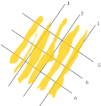
Consider a region or volume containing two phases (solid and space), both having complex architecture, such as a region of trabecular bone. We can study this volume to determine isotropy. If the volume is isotropic, then a line passing through the volume at any 3D orientation will make a similar number of intercepts through the solid phase. A bag of marbles would be isotropic. However a packet of spaghetti would be non-isotropic, or anisotropic, since lines going along the direction of the spaghetti would make few intercepts along the spaghetti rods while lines crossing at right-angles would make many intercepts. Figure 1 illustrates the difference in the number of intercepts for lines from different directions through an anisotropic, aligned group of structures.

Mean intercept length (MIL) analysis measures isotropy (it is usual to talk of measurement of the negative quantity anisotropy). Mean intercept length is found by sending a line through a 3D image volume containing binarised objects, and dividing the length of the test line through the analysed volume by the number of times that the line passes through or

(13)

intercepts part of the solid phase. Note that in this MIL calculation the intercept length may correlate with object thickness in a given orientation but does not measure it directly. Therefore it will give an accurate result if analysing a volume containing a sufficiently large number of objects, but is not suitable for analysis of single or small numbers of objects. For the MIL analysis, a grid of test lines is sent through the volume over a large number of 3D angles. The MIL for each angle is calculated as the average for all the lines of the grid. The spacing of this grid can be selected in CT-analyser preferences (the “advanced” tab).

Figure 1. A group of aligned long structures has a high anisotropy: test lines make few intercepts through the solid objects in the direction of the long axis of the structures, but perpendicular to the structures the lines make many more intercepts (numbers of intercepts are shown for each line).

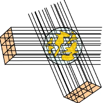
This requires that a spherical region is first defined within which the MIL analysis will be done and anisotropy measured, since the test lines must all cross the sphere centre and have an equal distribution of lengths, covering all 3D angles but distributed at random. In CT-analyser you can actually set a spherical volume of interest (VOI). However if a

(14)

Figure 2. For the MIL analysis, a grid of lines is sent through the volume over a large number of 3D angles (just two are illustrated here). The MIL for each angle is calculated as the average for all the lines of the grid.

The next step involves visualisation of the 3D distribution of MIL lengths as an ellipsoid. All the MIL lines are drawn passing through one point, and the length of each line is the bone phase MIL for that line. This process is called a polar plot of MIL. In 3D this creates a dense pin-cushion like effect with lines in all directions at different lengths. Figure 3 shows in a simple diagram the appearance of an MIL distribution in 3D. Any

asymmetry in the MILs with respect to 3D angle - which will represent the anisotropy of the bone in the spherical region - will make the line

distribution depart from an overall spherical shape and become elongated in the direction where the solid structures have the longest MIL (such as the axis of the spaghetti packet).

Clearly the MIL "pin-cushion" is a complex object, and a method is needed to extract some summary numerical parameters defining the orientation and isotropy / anisotropy of the MIL distribution. This is where the

anisotropy tensor analysis steps in. (Tensor means matrix.) This method is probably best attributed to Harrigan and Mann (1984) and describes the MIL distribution as an ellipsoid. An ellipsoid is a 3D ellipse.

As shown in figure 1, an ellipsoid has three axes. These describe the longest orientation, and the length and width (major and minor axes) of the ellipse section at right-angles to the longest orientation. The ellipsoid can be asymmetric in one axis only, like a rugby ball, or in two axes, like a bar of soap.

(15)

Figure 3. An ellipsoid (3D ellipse) is fitted to the 3D distribution of MILs (mean intercept lengths) measured over a full range of 3D stereo-angles. This ellipsoid is fitted statistically and has 3 vectors which are orthogonal (at right-angles to each other). A tensor (matrix) of 9 (3x3) eigenvectors describes the directions of the three vectors.

An ellipsoid is fitted to the MIL “pin-cushion” 3D polar plot. This is a statistical fit, finding the ellipsoid which most closely describes the 3D shape of the MIL distribution. MIL analysis therefore also outputs values indicating the strength of fit of the ellipsoid and associated error, such as the correlation coefficients.

A tensor or matrix is a way of describing an ellipse by a 3x3 matrix of numbers. Technically this is a second order tensor. The tensor describing the anisotropy ellipsoid is an orthogonal tensor, since it describes the ellipsoid axes which are orthogonal (at right angles) to each other. The end result of the anisotropy tensor analysis is the eigen analysis, eigen meaning characteristic. This comes in two parts. You have the 3x3 matrix of eigenvectors which describe the 3D angles of the three axes of the ellipsoid as described above - one column of 3 numbers for each vector. And the three eigenvalues are each an index of the relative MIL values (distance between bone intercepts) in each of the three axes described by the eigenvectors.

Finally, you can derive from the tensor eigen analysis a single parameter measuring anisotropy: this is the degree of anisotropy (DA), and is traditionally expressed as the maximum eigenvalue divided by the minimum eigenvalue. Values for DA calculated in this way vary from 1 (fully isotropic) to infinity (fully anisotropic). Mathematically this is a cumbersome scale. A more convenient mathematical index of anisotropy is calculated as:

Vector 1 Vector 2

(16)

              eigenvalue eigenvalue DA max min 1

Here DA is 0 for total isotropy and 1 for total anisotropy. (Both values are reported by CT-analyser).

Nomenclature

General Scientific Bone ASBMR

Parameter name

Eigenvalues 1,

2, 3

Eigenvalues 1,

2, 3

Parameter symbol none

none

Unit

none

The three eigenvalues are each an index of the relative MIL values

(distance between intercepts) in each of the three directions of the three MIL analyses. These three directions are also expressed as the

eigenvectors, and are orthogonal to each other.

Nomenclature

General Scientific Bone ASBMR

Parameter name

Fractal

dimension

Fractal

dimension

Parameter symbol FD

FD

Unit

none

Fractal dimension is an indicator of surface complexity of an object, which quantifies how that object’s surface fills space. For examples of fractal objects, “fractal art” is abundant on the internet. True fractal objects have surface shapes which are repeated over many spatial scales. So the closer you look (i.e. the higher the magnification or “zoom in”) the more self-similar structure you see. A typical example is a fern leaf in which each side-branch is very similar to the whole fern leaf, and likewise each side-finger of each side branch also looks the same as the whole fern leaf, and so on. A true fractal object essentially has fractional, non-integer dimension, i.e. a line “trying” to fill a plane, or a plane trying to fill a 3D space, having dimension somewhere between 2 and 3.

(17)

Fractal dimension is calculated using the Kolmogorov or “box counting” method. It is calculated in both 2D and 3D in Skyscan CT-analyser. For the 3D calculation of FD, the volume is divided into an array of equal cubes, and the number of cubes containing part of the object surface is counted. This is repeated over a range of cube sizes such as 2-100 pixels. The number of cubes containing surface is plotted against cube length in a log-log plot, and the fractal dimension is obtained from the slope of the log-log regression. Fractal characteristics of trabecular bone, and methods for measurement of fractal dimension, are discussed by Chappard et al.

(2001).

For more details on fractal dimension please refer to:

http://en.wikipedia.org/wiki/Fractal_dimension

Nomenclature

General Scientific Bone ASBMR

Parameter name

Number of

objects

Number of

objects

Parameter symbol N. Obj.

N. Obj.

Unit

none

The total number of discreet binarised objects within the VOI is reported. A discreet 3D object is a connected assemblage of solid (white) voxels fully surrounded on all sides in 3D by space (black) voxels.

Nomenclature

General Scientific Bone ASBMR

Parameter name

Number of

Closed Pores

Number of

Closed Pores

Parameter symbol Po.N(cl)

Po.N(cl)

Unit

none

The total number of discreet binarised closed pores within the VOI is reported. A closed pore in 3D is a connected assemblage of space (black) voxels that is fully surrounded on all sides in 3D by solid (white) voxels.

(18)

Nomenclature

General Scientific Bone ASBMR

Parameter name

Volume of

Closed Pores

Volume of

Closed Pores

Parameter symbol Po.V(cl)

Po.V(cl)

Unit

mm

3

_mm

3

The total volume of all closed pores within the VOI, as defined above (under “number of closed pores”) is reported.

Nomenclature

General Scientific Bone ASBMR

Parameter name

Surface of

Closed Pores

Surface of

Closed Pores

Parameter symbol Po.S(cl)

Po.S(cl)

Unit

mm

2

mm

2

The total surface area of all closed pores within the VOI, as defined above (under “number of closed pores”) is reported.

Nomenclature

General Scientific Bone ASBMR

Parameter name

Closed Porosity

(percent)

Closed Porosity

(percent)

Parameter symbol Po

Po

Unit

%

Percent closed porosity is the volume of closed pores (as defined above) as a percent of the total of solid plus closed pore volume, within the VOI. (Please note – this is a “material porosity”, and is calculated differently from of open porosity and total porosity, where the denominator is total VOI volume.)

(19)

Nomenclature

General Scientific Bone ASBMR

Parameter name

Volume of Open

Pore Space

Volume of Open

Pore Space

Parameter symbol Po.V(op)

Po.V(op)

Unit

mm

3

_mm

3

The total volume of all open pores within the VOI, is reported. An open pore is defined as any space located within a solid object or between solid objects, which has any connection in 3D to the space outside the object or objects.

Nomenclature

General Scientific Bone ASBMR

Parameter name

Open Porosity

(percent)

Open Porosity

(percent)

Parameter symbol Po(op)

Po(op)

Unit

%

Percent open porosity is the volume of open pores (as defined above) as a percent of the total VOI volume.

Nomenclature

General Scientific Bone ASBMR

Parameter name

Total Volume of

Pore Space

Total Volume of

Pore Space

Parameter symbol Po.V(tot)

Po.V(tot)

Unit

mm

3

_mm

3

(20)

Nomenclature

General Scientific Bone ASBMR

Parameter name

Total Porosity

(percent)

Total Porosity

(percent)

Parameter symbol Po(tot)

Po(tot)

Unit

%

Total porosity is the volume of all open plus closed pores (as defined above) as a percent of the total VOI volume.

Nomenclature

General Scientific Bone ASBMR

Parameter name

Euler number

Parameter symbol EN

EN

Unit

none

The calculation of Euler number in 3D is based on software code kindly provided by Erasmus University, Rotterdam, The Netherlands (Dr Erwin Waarsing) using the Conneulor method from Aarhus University, Denmark (Dr. Anders Odgaard; see Gunderson et. al. 1993).

Note also that up to CTAn version 1.9.3.2 Euler number was calculated in the 2D analysis only (both in the integrated and individual object 2D analyses) . From CTAn version 1.9.3.3 onwards Euler connectivity and number are also calculated in 3D, and included in the standard

(integrated) 3D analysis.

The Euler-Poincare number –abbreviated to “Euler number” – is an

indicator of connectedness of a 3D complex structure. The Euler number is characteristic of a three-dimensional structure which is topologically

invariant (it is unchanged by inflation or compression or distortion of the structure). It measures what might be called “redundant connectivity” – the degree to which parts of the object are multiply connected (Odgaard

et al. 1993). It is a measure of how many connections in a structure can be severed before the structure falls into two separate pieces.

(Topologically the object can be compressed into a sphere and the

redundant connections appear as “handles”.) The components of the Euler number are the three Betti numbers: 0 is the number of objects, 1 the

connectivity, and 2 the number of enclosed cavities. The Euler-Poincare

formula for a 3D object X is given:

2 1 0

)

(





X







(21)

Euler analysis provides a measure of connectivity density, indicating the number of redundant connections between trabecular structures per unit volume. Trabecular connectivity can contribute significantly to structure strength (Odgaard 1997). One useful and fast algorithm for calculating the Euler connectivity in 3D is the “Conneulor” (Gunderson et al. 1993).

(22)

A2: 3D morphometric parameters calculated for all

individual binarised 3D object within the volume of

interest (VOI)

Nomenclature

General Scientific Bone ASBMR

Parameter name

Object volume

Bone volume

Parameter symbol Obj.V

BV

Unit

mm

3

_mm

3

General Scientific Bone ASBMR

Parameter name

Centroids X, Y, Z Centroids X, Y, Z

Parameter symbol Crd.X, CrdY, CrdZ Crd.X, CrdY, CrdZ

Unit

mm

The centroid is the XYZ coordinate of the average Cartesian vectorial position of each discreet 3D object, within the VOI.

(24)

Nomenclature

General Scientific Bone ASBMR

Parameter name

Structure model

index

Structure model

index

Parameter symbol SMI

SMI

Unit

Structure model index indicates the relative prevalence of rods and plates in a 3D structure such as trabecular bone. SMI involves a measurement of surface convexity. Ideal values of SMI for an exact rectangular plate, cylinder and sphere are 0, 3 and 4 respectively. (Conversely, cylindrical and spherical cavities have SMI of -3 and -4 respectively.)

The calculation of SMI is based on dilation of the 3D voxel model, that is, artificially adding one voxel thickness to all binarised object surfaces (Hildebrand et al. 1997b). SMI is derived as follows:

        6 '₂ S V S SMI

where S is the object surface area before dilation and S’ is the change in surface area caused by dilation. V is the initial, undilated object volume. It should be noted that concave surfaces of enclosed cavities represent negative convexity to the SMI parameter, since dilation of an enclosed space will reduce surface area causing S’ to be negative. Therefore regions of a solid (such as bone) containing enclosed cavities – such as regions with relative volume above 50% – can have negative SMI values. As a consequence, the SMI parameter is sensitive to percent volume. Note also that artificial corners and edges created by the intersection of an object with the volume of interest boundary will also affect the measured SMI, increasing its value.

Nomenclature

General Scientific Bone ASBMR

Parameter name

Volume-equivalent

sphere diameter

Volume-equivalent

sphere diameter

Parameter symbol ESDv

ESDv

Unit

mm

The diameter of the sphere that would have the same volume as the discreet 3D object. ESDv is expressed:

(25)

√

where V is the object volume.

Nomenclature

General Scientific Bone ASBMR

Parameter name

volume-equivalent sphere will be much smaller than the particle surface area, thus

Sph will be low. The maximum value possible is 1, which would be obtained for a sphere.

A Wikipedia entry on Sph is at:

(27)

B: 2D MORPHOMETRIC PARAMETERS

B1: 2D morphometric parameters calculated

“slice-by-slice”, integrated for the whole volume of

interest (VOI)

Nomenclature

General Scientific Bone ASBMR

Parameter name

Total VOI

volume

Tissue volume

Parameter symbol TV

TV

Unit

mm

3

_mm

3

Total volume of the volume-of-interest (VOI). The 2D measurement is the total number of voxels of (solid and space) in the VOI times the voxel volume. Please note that in the case of Bone ASBMR nomenclature, the word “tissue” refers to the volume of interest. It does not mean any kind of recognition of any particular density range as biological tissue, soft, hard or otherwise.

Nomenclature

General Scientific Bone ASBMR

Parameter name

Object volume

Bone volume

Parameter symbol Obj.V

BV

Unit

mm

3

_mm

3

Total volume of binarised objects within the VOI. The 2D measurement is equal to the number of voxels of binarised solid objects within the VOI times the voxel volume.

(28)

Nomenclature

General Scientific Bone ASBMR

Parameter name

Percent volume Percent bone

volume

Parameter symbol Obj.V/TV

BV/TV

Unit

%

The percentage of the VOI occupied by binarised solid objects. This

parameter is only relevant if the studied volume is fully contained within a well-defined biphasic region of solid and space, such as a trabecular bone region, and does not for example extend into or beyond the boundary of the object – such as the cortical boundary of a bone sample. The

meaningfulness of measured percent volume depends on the criteria applied in selecting the volume of interest. Where the ROI / VOI

boundaries are loosely drawn in the surrounding space around an object for instance, then % object volume has no meaning.

Nomenclature

General Scientific Bone ASBMR

Parameter name

VOI surface

Tissue surface

Parameter symbol TS

TS

Unit

mm

2

_mm

2

The surface area of the volume of interest, measured in 2D, using the Pratt algorithm (Pratt 1991). Note that there are two components to

surface measured in 2D for a 3D multilayer dataset; first the perimeters of the binarised objects on each crossectional level, and second, the vertical surfaces exposed by pixel differences between adjacent crossections.

Nomenclature

General Scientific Bone ASBMR

Parameter name

Object surface

Bone surface

Parameter symbol Obj.S

BS

Unit

mm

2

_mm

2

The surface area of all the solid objects within the VOI, measured in 2D, using the Pratt algorithm (Pratt 1991). Note that there are two

components to surface measured in 2D for a 3D multilayer dataset; first the perimeters of the binarised objects on each crossectional level, and

(29)

second, the vertical surfaces exposed by pixel differences between adjacent crossections.

Nomenclature

General Scientific Bone ASBMR

Parameter name

Object surface /

volume ratio

Bone surface /

volume ratio

Parameter symbol Obj.S/Obj.V

BS/BV

Unit

mm

-1

_mm

-1

The ratio of solid surface to volume (both as defined above) measured in 2D within the VOI. Surface to volume ratio or “specific surface” is a useful basic parameter in characterising the complexity of structures.

Nomenclature

General Scientific Bone ASBMR

Parameter name

Mean total

crossectional

ROI area

Mean total

crossectional

tissue area

Parameter symbol T.Ar

T.Ar

Unit

mm

2

_mm

2

The mean of the crossectional ROI area for all slices in the selected range of the VOI. Note that by using the “shrink-wrap” function, the ROI

boundary can become effectively the outer boundary of the object, while not including any internal spaces or structure in the measurement. This allows for example measurement of inner and outer surfaces of porous or hollow objects, such as the periosteal (outer) and endosteal (inner)

(30)

Nomenclature

General Scientific Bone ASBMR

Parameter name

Mean total

crossectional

ROI perimeter

Mean total

crossectional

tissue perimeter

Parameter symbol T.Pm

T.Pm

Unit

mm

The mean of the crossectional ROI perimeter for all slices in the selected range of the VOI. Note that by using the “shrink-wrap” function, the ROI perimeter can become effectively the outer perimeter of the object, while not including any internal spaces or structure in the measurement. This allows for example measurement of inner and outer surfaces of porous or hollow objects.

Nomenclature

General Scientific Bone ASBMR

Parameter name

Mean total

crossectional

object area

Mean total

crossectional

bone area

Parameter symbol Obj.Ar

B.Ar

Unit

mm

2

_mm

2

The mean of the crossectional object or bone area for all slices in the selected range of the VOI.

Nomenclature

General Scientific Bone ASBMR

Parameter name

_mm

2

The mean area of discreet 2D objects in a single crossectional image slice. This parameter can be an indicator of structural connectivity – in

interconnected structures (e.g. trabecular bone or other networks, scaffolds or foams) high connectivity results in highly interconnected objects which are few in number in a single crossection – by contrast fragmentation results in larger numbers of smaller objects (for application of this parameter to bone morphometry see for example Vermeirsch et al.

(32)

Nomenclature

General Scientific Bone ASBMR

Parameter name

Average object

equivalent circle

diameter per

slice

Average object

equivalent circle

diameter per

slice

Parameter symbol Av.Obj.ECD

Av.Obj.ECD

Unit

mm

The mean equivalent circle diameter of all discreet 2D objects in a single crossectional image slice, defined as the diameter of the equivalent circle having the same area as the measured object.

Nomenclature

General Scientific Bone ASBMR

Parameter name

Mean polar

moment of

inertia

Mean polar

moment of

inertia

Parameter symbol MMI(polar)

MMI(polar)

Unit

mm

4

_mm

4

This 2D crossectional function is a basic strength index and indicates the resistance to rotation of a crossection about a chosen axis (assuming uniform material stress-strain strength properties).

Moment of inertia is the rotational analogue of mass for linear motion and must be specified with respect to a chosen axis of rotation. For a point mass (represented by an image pixel) the moment of inertia (I) is simply the mass (m) times the square of perpendicular distance (r) to the

rotation axis, I = mr2_{. Moment of inertia for a crossection – for example of}

cortical bone – is the integral of all the solid (bone) pixels. For more detail on moment of inertia please refer to:

(33)

Nomenclature

General Scientific Bone ASBMR

Parameter name

Mean

eccentricity

Mean

eccentricity

Parameter symbol Ecc

Ecc

Unit

(none)

Eccentricity is a 2D shape analysis of discreet binarised objects. Objects are approximated as ellipses, and

eccentricity is an elliptic parameter indicating departure from circular shape by lengthening (a circle is an ellipse with an eccentricity of zero). An ellipse is defined as having two focal points (F1 and F2), a centre (C) and major and minor axes. The major axis is defined as 2a where a is the “semi major axis”; likewise, 2b is the minor axis. Eccentricity e is a function of the (semi)major and minor axes such that: 2 2

1 a

b

e





Higher eccentricity means generally elongated objects, while decreased values means an approach toward circular shape.

Nomenclature

General Scientific Bone ASBMR

Parameter name

Crossectional

thickness

Crossectional

thickness

Parameter symbol Cs.Th

Cs.Th

Unit

mm

Crossectional thickness is calculated in 2D on the basis of the plate model where Th = 2 / (surface/volume) . Surface in 2D integrated “slice-by-slice” analysis is calculated as described above (Obj.S) from both horizontal and vertical pixel boundaries. Crossectional thickness is a calculation of thickness in which the vertical surfaces, between pixels of adjacent crossections, are excluded; only the perimeters of crossections are used to calculate surface. This definition of surface excludes error caused by large artificially cut surfaces that sometimes occur at the top

(34)

and bottom of VOIs, such as a VOI representing a short section of cortical bone with large exposed crossections at each end. (By contrast, the “structure thickness” or “trabecular thickness” 2D parameters – below – include surface measured both vertically and horizontally: thus this latter thickness calculation yields smaller thickness values.)

Nomenclature

General Scientific Bone ASBMR

Parameter name

Structure

thickness (plate

and rod models)

Trabecular

thickness (plate

and rod models)

Parameter symbol St.Th (pl) or (rd) Tb.Th(pl) or (rd)

Unit

mm

Calculation – or estimation – of St.Th or Tb.Th from 2D measurements requires an assumption about the nature of the structure (a “structural model”). Three simple structure models, the parallel plate, the cylinder rod and the sphere model, provide the range of values within which a hypothetical “true” thickness will be located. Thickness defined by these models (Parfitt et al. 1987) is given:

Parallel plate model:



BS BV



Th Tb / 2 . 

Cylinder rod model:



BS BV



Th Tb / 4 .  Sphere model:



BS BV



Th Tb / 6 . 

Where BS/BV is the surface to volume ratio, mm-1_.

Note that for the above equations, if the surface measurements are made from one or a few 2D crossectional slices (such as in histological analysis), then the numerator (2, 4 or 6) should be divided by a correction factor of 1.199. This approximates a correction from 2D to 3D. However as

(35)

CT-analyser includes vertical surfaces between solid and space voxels in adjacent image slices. It is thus in fact an essentially 3D measurement based on a simple cubic voxel model. Therefore the thickness model based estimated should not here include the 1.199 correction factor.

Nomenclature

General Scientific Bone ASBMR

Parameter name

Structure

separation

(plate and rod

models)

Trabecular

separation

(plate and rod

models)

Parameter symbol Sr.Sp

Tb.Sp

Unit

mm

Trabecular separation is essentially the thickness of the spaces as defined by binarisation within the VOI. It can also be calculated from 2D images with model assumptions. Applying the structural models as for thickness, structure separation is calculated:

Parallel plate model:

Th Tb N Tb Sp Tb . . 1 .       

Cylinder rod model:

                        1 4 . . BV TV Dm Tb Sp Tb



where TV is total volume of VOI and BV is bone (or solid) volume (Parfitt

et al. 1987). Note that each of the above definitions takes the Tb.Th (or Tb.Dm) value derived from the corresponding plate or rod model.

(36)

Nomenclature

General Scientific Bone ASBMR

Parameter name

Structure linear

density (plate

and rod models)

Trabecular

number (plate

and rod models)

Parameter symbol St.Li.Dn(pl)

Tb.N

Unit

mm

-1

_mm

-1

Structure linear density or trabecular number implies the number of traversals across a solid structure, such as a bone trabecula, made per unit length by a random linear path through the volume of interest (VOI). Plate and rod model 2D-based definitions of Tb.N again take the

corresponding Tb.Th values: Parallel plate model:

Th

Tb

TV

BV

N

Tb

.

)

/

(

.



Cylinder rod model:

Dm Tb TV BV N Tb . 4 .              



Nomenclature

General Scientific Bone ASBMR

Parameter name

Fragmentation

index

Trabecular bone

pattern factor

Parameter symbol Fr.I

Tb.Pf

Unit

mm

-1

_mm

-1

This is an inverse index of connectivity, which was developed and defined by Hahn et al. (1992) for application to trabecular bone. It was applied by these authors originally to 2D images of trabecular bone, and it calculates an index of relative convexity or concavity of the total bone surface, on the principle that concavity indicates connectivity (and the presence of “nodes”), and convexity indicates isolated disconnected structures (struts). Tb.Pf is calculated in 2D by comparing area and perimeter of binarised solid before and after a single voxel image dilation. It is defined:

(37)

         2 1 2 1 . A A P P Pf Tb

Where P and A are the solid perimeter and area, respectively, and the subscript numbers 1 and 2 indicate before and after image dilation. Structural / trabecular connectedness results in enclosed spaces and concave perimeters, and dilation of such perimeters will contract them, resulting in reduced perimeter. By contrast, open ends or nodes which have convex perimeters will have their surface expanded by surface dilation, thus causing increased perimeter. As a result, lower Tb.Pf signifies better connected trabecular lattices while higher Tb.Pf means a more disconnected trabecular structure. A prevalence of enclosed cavities and concave surfaces can push Tb.Pf to negative values. This parameter is best considered as a relative index for comparing different scanned

objects; its absolute value does not have much meaning.

Nomenclature

General Scientific Bone ASBMR

Parameter name

Closed Porosity

(percent)

Closed Porosity

(percent)

Parameter symbol Po(cl)

Po(cl)

Unit

%

Closed porosity is measured in the 2D slice-by-slice analysis in

CT-analyser. Binarised objects are identified containing fully enclosed spaces, and closed porosity is the area of those spaces as a percent of the total area of binarised objects. Note that the denominator of total object area includes the closed pores. Closed porosity measurement ignores space which is not fully surrounded by solid. Note – closed porosity in 2D is usually much larger than the equivalent parameter measured in 3D; a space region is more likely to be surrounded by solid in a single

(38)

Nomenclature

General Scientific Bone ASBMR

Parameter name

Centroids X, Y, Z Centroids X, Y, Z

Parameter symbol Crd.X, CrdY, CrdZ Crd.X, CrdY, CrdZ

Unit

mm

The centroid is the XYZ coordinate of the average Cartesian vectorial position of all voxels within the VOI.

Nomenclature

General Scientific Bone ASBMR

Parameter name

Fractal

dimension

Fractal

dimension

Parameter symbol FD

FD

Unit

none

Fractal dimension is an indicator of surface complexity of an object, which quantifies how that object’s surface fills space. For examples of fractal objects, “fractal art” is abundant on the internet. True fractal objects have surface shapes which are repeated over many spatial scales. So the closer you look (i.e. the higher the magnification or “zoom in”) the more self-similar structure you see. A typical example is a fern leaf in which each side-branch is very similar to the whole fern leaf, and likewise each side-finger of each side branch also looks the same as the whole fern leaf, and so on. A true fractal object essentially has fractional, non-integer dimension, i.e. a line “trying” to fill a plane, or a plane trying to fill a 3D space, having dimension somewhere between 2 and 3.

Fractal dimension is calculated using the Kolmogorov or “box counting” method. It is calculated in both 2D and 3D in Skyscan CT-analyser. For 2D calculation of FD, the crossection image is divided into an array of equal squares, and the number of squares containing part of the object surface is counted. This is repeated over a range of square sizes such as 2-100 pixels. The number of squares containing surface is plotted against square length in a log-log plot, and the fractal dimension is obtained from the slope of the log-log regression. Fractal characteristics of trabecular bone, and methods for measurement of fractal dimension, are discussed by Chappard et al. (2001). Fractal dimension is a useful indicator of complexity in structures.

(39)

Nomenclature

General Scientific Bone ASBMR

Parameter name

Intersection

surface

Intersection

surface

Parameter symbol i.S

i.S

Unit

mm

2

_mm

2

Intersection surface is the surface of the ROI intersected by solid binarised objects, that is, the part of the ROI boundary surface that runs through solid objects. This parameter is useful, for example, in evaluating bone growth at a fixed distance away from an orthopaedic bone implant. The intersection surface is calculated for each separate crossection level, but is also integrated over all VOI levels in the data summary at the head of the 2D analysis report. Note that the intersection surface calculated in 2D does not include vertical (between-crossection) surfaces, only perimeters of objects within crossections. This can make the 2D calculation of i.S. useful for excluding artificial cut surfaces at the top and bottom of the VOI, as was discussed for the parameter crossectional thickness.

(40)

B2: 2D morphometric parameters calculated for

each individual binarised 2D object within the

region of interest (ROI) for the single selected

image level only

Nomenclature

General Scientific Bone ASBMR

Parameter name

Area

Parameter symbol Ar

Ar

Unit

mm

2

mm

2

The area of the individual 2D object, calculated using the Pratt algorithm (Pratt 1991).

Nomenclature

General Scientific Bone ASBMR

Parameter name

Perimeter

Parameter symbol Pm

Pm

Unit

mm

The perimeter of the individual 2D object, calculated using the Pratt algorithm (Pratt 1991).

Nomenclature

General Scientific Bone ASBMR

Parameter name

Form factor

Parameter symbol FF

FF

Unit

none

The form factor of the individual 2D object. FF is calculated by the equation below:          4 ₂ Pm A FF



(41)

where A and Pm are object area and perimeter respectively. Elongation of individual objects results in smaller values of form factor.

Nomenclature

General Scientific Bone ASBMR

Parameter name

Area Equivalent

Circle Diameter

Area Equivalent

Circle Diameter

Parameter symbol ECDa

ECDa

Unit

mm

The area-equivalent circle diameter of a discreet 2D object is defined as the diameter of the circle having the same area as the measured object. It is calculated as

√

where A is the area of the object.

Nomenclature

General Scientific Bone ASBMR

Parameter name

Roundness

Parameter symbol R

R

Unit

none

Roundness of a discreet 2D object is defined as:

( ( ) )

where A is the object area. The value of R ranges from 0 to 1, with 1 signifying a circle.

(42)

Nomenclature

General Scientific Bone ASBMR

Parameter name

Euler number

Parameter symbol EN

EN

Unit

none

The Euler-Poincare – or the abbreviated “Euler number” – is also an indicator of connectedness of a complex object. The Euler number

measures what might be called “redundant connectivity” – the degree to which parts of the object are multiply connected (Odgaard et al. 1993). It is a measure of how many connections in a structure can be severed before the structure falls into two separate pieces. (Topologically the object can be compressed into a circle and the redundant connections appear as “handles”.) The components of the Euler number are the three Betti numbers: 0 is the number of objects, 1 the connectivity, and 2 the

number of enclosed cavities. The Euler-Poincare formula for a 3D object X is given: 2 1 0

)

(





X







In calculating the Euler number of an individual object,



₀will always be 1. The values of



₁ and



₂will therefore determine the single object’s Euler number.

Nomenclature

General Scientific Bone ASBMR

Parameter name

Porosity

Parameter symbol Po

Po

Unit

%

Porosity for individual objects in 2D is defined as closed porosity as described elsewhere – the volume of any spaces fully surrounded in the given crossectional plane by solid, as a percent of the volume of solid plus closed pores.