Uncertainty reduction and parameters estimation of a~distributed hydrological model with ground and remote sensing data

(1)

HESSD

11, 6215–6271, 2014 Hydrological model parameters uncertainty reduction F. Silvestro et al. Title Page Abstract Introduction Conclusions References Tables Figures J I J I Back Close

Full Screen / Esc Printer-friendly Version Interactive Discussion Discussion P a per | Discus sion P a per | Discussion P a per | Discussion P a per |

Hydrol. Earth Syst. Sci. Discuss., 11, 6215–6271, 2014 www.hydrol-earth-syst-sci-discuss.net/11/6215/2014/ doi:10.5194/hessd-11-6215-2014

This discussion paper is/has been under review for the journal Hydrology and Earth System Sciences (HESS). Please refer to the corresponding final paper in HESS if available.

Uncertainty reduction and parameters

estimation of a distributed hydrological

model with ground and remote sensing

data

F. Silvestro1, S. Gabellani1, R. Rudari1, F. Delogu1, P. Laiolo1, and G. Boni1,2

1

CIMA Research Foundation, Savona, Italy

2

DIBRIS, University of Genova, Genova, Switzerland

Received: 14 May 2014 – Accepted: 15 May 2014 – Published: 13 June 2014 Correspondence to: F. Silvestro ([email protected])

(2)

HESSD

Full Screen / Esc Printer-friendly Version Interactive Discussion Discussion P a per | Discus sion P a per | Discussion P a per | Discussion P a per | Abstract

During the last decade the opportunity and usefulness of using remote sensing data in hydrology, hydrometeorology and geomorphology has become even more evident and clear. Satellite based products often provide the advantage of observing hydrologic variables in a distributed way while offering a different view that can help to understand

5

and model the hydrological cycle. Moreover, remote sensing data are fundamental in scarce data environments. The use of satellite derived DTM, which are globally available (e.g. from SRTM as used in this work), have become standard practice in hydrologic model implementation, but other types of satellite derived data are still underutilized.

10

In this work, Meteosat Second Generation Land Surface Temperature (LST) estimates and Surface Soil Moisture (SSM) available from EUMETSAT H-SAF are used

to calibrate the Continuum hydrological model that computes such state variables in

a prognostic mode. This work aims at proving that satellite observations dramatically reduce uncertainties in parameters calibration by reducing their equifinality. Two

15

parameter estimation strategies are implemented and tested: a multi-objective approach that includes ground observations and one solely based on remotely sensed data.

Two Italian catchments are used as the test bed to verify the model capability in reproducing long-term (multi-year) simulations.

20

1 Introduction

The estimation of parameters in hydrological models is still an open issue in hydrology. Many works have been devoted to determining the best calibration strategy (Yapo et al., 1998; Madesen, 2000; Kim et al., 2007; Singh and Bardossy, 2012; Xu et al., 2013) with some trying to evaluate the uncertainties associated with the parameters

25

(3)

HESSD

Georgakakos, 2006; Zappa et al., 2010). This issue has become even more complex with the increasing use of complete and distributed hydrological models. This trend led to a significantly increase number of parameters that need calibration. A large number of parameters allows good performance in the calibration phase, but this can lead to a large number of equifinal parameter sets (Beven and Binley, 1992) sometimes

5

hampering the forecast ability of the models.

Traditionally, the calibration of hydrological models requires appropriate series of historical data, particularly of stream flow data, which are not easily available everywhere in the world. Such issues raised the attention of the scientific community becoming the focus of coordinated scientific initiatives (e.g. Prediction in Ungauged

10

Basin (PUB), science initiative of the International Association of Hydrological Sciences, that was developed in the period 2003–2012). In a world where the data sharing capacity is exponentially increasing, it seems that the problem of data shortage for hydrologic calibration would not disappear as gaging stations and access to river discharge information have been declining since the 1980s (Vörösmarty et al., 2001).

15

As a consequence, the use of remote sensing for direct stream flow measurements has received increased attention lately and even if promising in some cases, it faces various technological, physical and scale limits. The more straightforward approaches use statistical relationships between remotely sensed river widths and in situ measurements (Brakenridge et al., 2005; Pavelsky, 2014) making them suitable

20

for the extension of existing historical data, but unusable for ungauged sites. The limits are mainly due to the fact that accurate estimates of stream flow require the availability of several hydraulic parameters (width, depth, slope, channel morphology), which are difficult to derive entirely from remote sensing. Simplified models that make use of some of these parameters introduce uncertainties that limit their applicability

25

(see e.g. Bjerklie et al., 2003). Additionally and independently of the specific technique utilized, the detection of changes in hydraulic parameters, and then on stream flows, has to deal with the spatiotemporal resolution of the satellite sensors. The models proposed in the literature (see Bjerklie et al., 2003 for a comprehensive review) are

(4)

HESSD

not suitable for detecting changes in discharge for small-scale basins, whose flow channels’ spatial scale is of the order of magnitude of the spatial resolution and have flood dynamics significantly faster than the temporal resolution of the sensors (Brakenridge et al., 2012).

Nowadays the remote sensing of other meteorological, hydrological and ecological

5

variables is more reliable and widely available at the global scale. Satellite products such as precipitation, Short Wave and Long Wave radiation, atmospheric profiles, vegetation parameters, Land Surface Temperature (LST), evapotranspiration (ET), and Digital Elevation Models are now operational and widely used in hydrological modeling. Experiments to understand the accuracy of these products are quite popular (see

10

e.g. Bitew and Gebremichael, 2011; Zhang et al., 2013; Murray et al., 2013; Yu et al., 2012; Göttsche and Hulley, 2012; Crow et al., 2012; Brocca et al., 2011a). These kinds of data are by now, available for a very high percentage of the earth’s surface, and cover most of the areas where the density of ground stations is poor. This leads to a panorama in which running a hydrological model by using only satellite information is

15

a real possibility (Silvestro et al., 2013). However, the ability to calibrate a model using satellite data, even in combination with traditional in situ data, is still a challenging topic. Scientific work in this field goes in many directions: Rhoads and Dunayah (2001) used satellite-derived LST to validate a land surface model, Caparrini and Castelli (2004) and Sini et al. (2008) assimilated remote sensed measurements into a

land-20

surface model to estimate the surface turbulent fluxes, Brocca et al. (2011a) analyzed different remote sensed soil humidity estimations with the perspective of using them in hydrological modeling, White and Lewis (2011) used satellite imagery to monitor the dynamics of wetlands of the Australian Great Artesian Basin, Khan et al. (2011) have recently proposed a procedure to calibrate a fully distributed hydrological model using

25

satellite-derived flood maps.

In the more formal context of hydrologic calibration, this work analyses the improved calibration skill of a distributed continuous hydrologic model by augmenting the model constraints with satellite-retrieved data. As a consequence, in the context of a classical

(5)

HESSD

uncertainty analysis (Beven and Binley, 1992; Shen et al., 2012) it is shown that the parameters’ uncertainty and equifinality can be reduced. After that two simple calibration methods were developed and applied in order to exploit the advantages of utilizing sensor observations. The first method lies in the family of the multi-objective calibration approaches (Efstratiadis and Koutsoyiannis, 2010) and tries to

5

exploit both satellite and streamflow data. The second method is an attempt to use only satellite data without any streamflow measurements, simulating the case of a basin in a scarce data environment. This last experiment is conceived along the lines of Silvestro et al. (2013), but with a more comprehensive approach that exploits both LST and soil humidity estimates from satellites.

10

The hydrological model used in the study is Continuum (Silvestro et al., 2013). It is a distributed continuous model conceived to satisfy the principle of parsimony in parameterization (Perrin et al., 2001; Coccia et al., 2009; Todini et al., 2009; Efstratiadis and Koutsoyiannis, 2010) and to be balanced between a good representation of physical processes and the simplicity of the schematizations and implementation.

15

From a more generic point of view, this work proposes to focus the attention of the modeling community to the need for investment in augmenting the number of observable state variables, with a specific focus on distributed variables. This paradigm aims at increasing the parameters’ identifiability and improving model structure analysis.

20

The article is organized as follows: Sect. 2 provides a short overview of the

Continuumhydrological model, Sect. 3 describes the data set used for the study and Sect. 4 shows the uncertainty analysis of the most sensitive model parameters. The proposed calibration process with the analysis of the results is presented in Sects. 5 and 6. Section 7 contains discussion and conclusions.

(6)

HESSD

Full Screen / Esc Printer-friendly Version Interactive Discussion Discussion P a per | Discus sion P a per | Discussion P a per | Discussion P a per | 2 Model overview

Continuumis a continuous distributed hydrological model that relies on a morphological approach, based on drainage network components identification (Giannoni et al., 2000, 2005). These components are derived from DEMs. The DEM resolution drives the model spatial resolution. Flow in the soil is divided firstly into a sub-surface flow

5

component that is based on a modified Horton schematization (see Gabellani et al., 2008 for details) and that follows the drainage network directions; and secondly, into a deep flow component that moves following the hydraulic head gradient obtained by the water-table modeling. The surface flow schematization distinguishes between channel and hillslope flows. The overland flow (hillslopes) is described by a linear

10

reservoir scheme, while for the channel flow (channel) a schematization derived by the kinematic wave approach (Wooding, 1965; Todini and Ciarapica, 2002) is used. The energy balance is solved explicitly at cell scale by means of the force-restore equation, that allows having the LST as a distributed state variable of the model (e.g., Lin, 1980; Dickinson, 1988; Sini et al., 2008). For further details on the model please refer to

15

Silvestro et al. (2013).

Various authors highlighted the importance of reducing the model parameterization and maintaining a stable and simple structure (Montaldo et al., 2005; Coccia et al., 2009; Todini, 2009; Brocca et al., 2011b). The design of Continuum follows the philosophy of finding a balance between a detailed description of the physical

20

processes and a robust and parsimonious parameterization.

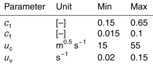
Continuum has six parameters that need calibration at basin scale: two for the surface flow, two for the sub-surface flow and two for deep flow and the water table.

In Table 1 the calibration parameters are listed and linked to the physical processes parameterized.

25

The hillslope flow motion parameter u_h influences the general shape of the

hydrograph, while the impact of u_c on the hydrograph shape depends on the length

(7)

HESSD

identifies the fraction of water volume in the soil that can be extracted only through

evapotranspiration. The “infiltration capacity” parameter c_f controls the velocity of

subsurface flow (i.e, it is related to saturated hydraulic conductivity). Both c_t and c_f

regulate the dynamics of saturation at cell scale. The parametersV_WmaxandR_f govern

the deep flow and the water table dynamic and have a reduced influence compared

5

to the other four parameters (Silvestro et al., 2013). This is due to the slow temporal dynamic of the water table. The sensitivity toR_fincreases with the total basin drainage

area when the effect of the interaction between the water table and the vadose zone

becomes crucial in the formation of the recession curve between the rainfall events. Continuum accounts for LST as an explicit state variable and allows for the estimation

10

of the soil moisture in the root zone as the saturation degree (sw) defined here by the

ratio of the actual soil water content and the maximum storage capacityV_Wmax. Both of

these variables are represented at DEM resolution.

2.1 Snow melting module

The snow accumulation-melting module was introduced in order to carry out multi-year

15

simulations in alpine climates. It is a simple model which is derived from commonly used equations (Maidment, 1992) and it is forced by meteorological observations.

The equations that describe the snow mass conservation and its melting are the following:

∆SWE

∆t =Sf−SM (1)

20

where SWE is the snow water equivalent, S_f is the solid precipitation and SM is the

snow melting estimated as:

SM= Rn

ρ_wλ_f +mc·(Ta−T0) (2)

(8)

HESSD

whereR_n is the net radiation, ρ_w the water density, λ_f the latent heat of melting, T_a

the air temperature.T and m_c are two parameters that represent the temperature at

which the melting starts and the melting coefficient, respectively. These two parameters

are estimated using values from the literature (Maidment, 1992), T=0◦C and m_c=

4 mm day−1.

5

The mass balance is applied at cell scale for the entire domain of the model, so that a snow cover map can be generated with the same resolution of the DEM. The energy balance and, as a consequence, the evapotranspiration are inhibited for those cells where snow cover is present.

The applied approach is very simple and neglects the heat exchanges between the

10

soil and the snow cover, but it is generally sufficient if the goal is the estimation of the snow contribution to the runoff, especially when the regime of the basin is not strongly influenced by snow melting.

The precipitation is partitioned into solid or liquid if the air temperature is below or above a fixed threshold.

15

3 Dataset

The first test case is the Orba basin that is located in the Apennine part of the Piemonte region (Italy). It has a total area of approximately 800 km2 and it is a tributary of the Tanaro river (Fig. 1).

The Piemonte and Liguria regions meteorological networks monitor the basin.

20

Data from rain gauges, thermometers, hygrometers, shortwave radiometers and anemometers are available with a temporal resolution of 1 h. Two stage-gauging stations are working with maintained stage-discharge rating curves; the two stations are located quite far one from each other along the river: Tiglieto in a head catchment

(drained area: 75 km2) and Casalcermelli near the basin outlet (drained areas:

25

(9)

HESSD

For this application, we extended the data set used in Silvestro et al. (2013). The chosen period starts from 1 June 2006 and ends on 31 December 2011. The first five months of 2006 are used as the model “warm-up” period.

The second test case is the Casentino basin (Fig. 1). It is a head catchment of the Arno river basin located in Tuscany. The watershed is located in the Central Apennines

5

with elevation that ranges between 200 and 1600 m a.s.l. The mountainous part of the basin is mainly covered by forest, while cultivated fields or zones with low vegetation primarily make-up the flat areas. Urban areas cover a low percentage of territory.

The two basins are only marginally impacted by snowfall and snow cover during winter.

10

The meteorological network of the Tuscany Region provides rainfall, air temperature, air humidity, solar radiation and wind speed and direction with temporal resolution of 1 h. Only one gauging station (Subbiano) is working with a maintained stage-discharge rating curve; the gauge is located in the flat area of the basin at about 10 km from the confluence of the Casentino River along the Arno River (drained area

15

670 km2). The period of simulation ranges from 1 June 2005 to 31 December 2011.

The first five months of 2005 are used to warm-up the model.

The remote sensing data employed to implement the mode and set additional constraints to the model parameters are:

1. The Istituto Geografico Militare (IGM) Digital Elevation Model (DEM) used to

20

extract the basin morphological parameters (http://www.igmi.org/prodotti/dati_ numerici/dati_matrix.php);

2. Land Surface Analysis Satellite Applications Facility (LSA-SAF) Land Surface Temperature (LST) product retrieved from Meteosat Second Generation (MSG) observations (landsaf.meteo.pt);

25

3. SM-OBS-1 Surface Soil Moisture retrieved from ASCAT (Wagner et al., 2013) and distributed within the EUMETSAT Satellite Application Facility on Support

(10)

HESSD

to Operational Hydrology and Water Management (H-SAF) program used as a benchmark to be compared with the model output (hsaf.meteoam.it);

4. LSA-SAF Leaf Area Index (LAI) to parameterize the vegetation cover.

LST estimations are provided by LSA SAF of EUMETSAT (EUMETSAT, 2009). LST data are available every 15 min with a spatial resolution of approximately 0.04 deg

5

(about 4.5 km) since 2009.

The H-SAF SM-OBS-1 product consists of European maps of large scale Surface Soil Moisture (SSM) retrieved from Advanced Scatterometer (ASCAT), the active microwave sensor, which flies onboard three polar orbiting Meteorological Operational (METOP) satellites. This product gives reliable soil moisture estimates across different

10

test sites in Europe, Americas and Africa (Brocca et al., 2010; Albergel et al., 2012). EUMETSAT makes the product available, from 3 June 2009, in near real-time with a spatial resolution of approximately 25 km.

Since this measure is referred to the first centimeters of soil, the Soil Water Index (SWI) method, developed by Wagner et al. (1999), was applied to SSM satellite data to

15

obtain an estimate of the saturation degree in the root zone. This method relies on the analytical solution of a differential equation assuming that the variation in time of the average value of the soil moisture profile is linearly related to the difference between the surface and the profile soil moisture values. In this study a simple recursive formulation of the method is used (Stroud, 1999; Albergel et al., 2008):

20

LAI maps were produced with temporal update of fifteen days as averaged values of daily LSA-SAF maps at spatial resolution of 0.04 deg. (EUMETSAT, 2008).

The model resolution is set equal to the DEM resolution. The temporal resolution is set to 1 h, the surface flow needs a finer time step for computational reasons and it was fixed to 30 s.

(11)

HESSD

Full Screen / Esc Printer-friendly Version Interactive Discussion Discussion P a per | Discus sion P a per | Discussion P a per | Discussion P a per | 4 Hydrological uncertainty

The issue of model parameter uncertainty has been one of the main themes of scientific discussions over the last thirty years. Many authors faced the problem following

different approaches (see e.g. Beven and Binley, 1992; Liu et al., 2005; Carpenter

and Georgakakos, 2006; Zappa et al., 2010), but it is widely accepted and recognized

5

that parameter uncertainty is inevitable and rarely an optimal set of parameters that allows the best performance of the model in every condition exists; generally, there are multiple sets of parameters able to give similar results and are therefore equivalent if the final aim is identified, that is the so-called equifinality (Savenije, 2001).

In this section, we will not carry out a full predictive uncertainty analysis, but we will

10

analyze the parameter uncertainty based on equifinal realizations obtained by a Monte Carlo experiment; some concepts of the GLUE method (Beven and Binley, 1992) are used similarly to what was done in Zappa et al. (2010) and Shen et al. (2012). Finally, we made reference to the work of Liu et al. (2005) in order to estimate the probability of parameter couples conditioned to the observations.

15

The experiment was done in the Orba basin by randomly varying the four most sensitive parameters of the model (Liu et al., 2005) (c_t,c_f,u_c,u_h, for Continuum, see Silvestro et al., 2013, for details) and generating a set of 3000 streamflow simulations for the sub-period 16 August 2006 to 30 September 2006. The parameters have been extracted from a multi-uniform distribution. The sub-period includes various streamflow

20

regimes. The sampling space of the four parameters was defined by combining the literature (Beven and Binley, 1991; Liu et al., 2005; Zappa et al., 2010; Shen et al., 2012) with the results of the preliminary sensitivity analysis done by Silvestro et al. (2013) and considerations on the role and physical meaning of the parameters themselves. In Table 2 the range of variability of the parameters is reported.

(12)

HESSD

The Nash–Sutcilffe (NS) coefficient was chosen as main likelihood function since it is one of the most widely used measures to evaluate model performances in hydrology:

NS=1− tmax X t=1 (Q_m(t)−Q_o(t))2 (Q_m(t)− hQ_oi)2 (3)

whereQ_m(t) andQ_o(t) are the modeled and observed streamflows at time,t.

5

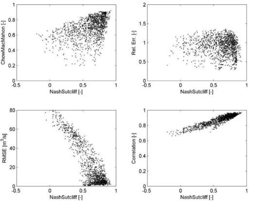
Four other scores were evaluated: Chiew–McMahon coefficient (CM, Chiew and

McMahon, 1994), Root Mean Square Error (RMSE), the correlation coefficient (CORR)

and the Relative Error (Rel. Err.). Each score can be influenced differently by different flow regimes and hydrograph characteristics, therefore for each simulation the NS was plotted against the other scores (Zappa et. al, 2010); the results are reported

10

in Fig. 2 and the graphs show that in all cases there are sets of behavioral parameters (Beven and Binley, 1992) that give similarly good values of the scores, indicating good simulation of the observed streamflow series.

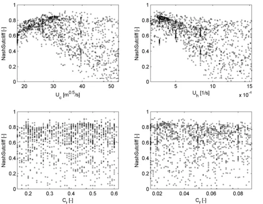
In Fig. 3, the dotty plots (Beven and Binley, 1992; Shen et al., 2012) of the four parameters are reported. Each graph shows the NS value as a function of the

15

parameter values. The variability of NS for a single parameter is quite high. In the case

of the two surface parametersu_c andu_h(upper subplots in the figure) a maximum for

NS can be identified, while forc_tandc_fthe behavior of NS is quite homogeneous for all the values in the physically acceptable range. This indicates thatu_c andu_hare closely linked to the streamflow simulation in the model, while the impact of c_f and c_t in the

20

discharge follows more complex paths, and it is hard to identify such parameters by matching the streamflow time series alone.

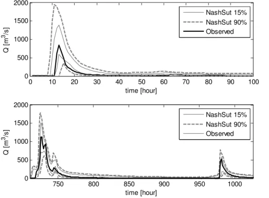
By sorting the discharge time series according to NS it is possible to evaluate the percentiles at each time step and show the uncertainty in terms of confidence intervals.

Simulations with NS lower than a fixed threshold (NS=0.4) did not behave according

25

to Shen et al. (2012). In Fig. 4, the 15 and 90 % confidence limits are reported for two time windows across the main streamflow events, which occurred in the considered period. The results show that the observed streamflow lays in the 90 % limit, therefore

(13)

HESSD

a parameter configuration that allows reproducing the flow observations exists at any time. Most of the hydrograph, and specifically the peak flow, lays in the 15 % limit. Part of the receding curve is not included showing some limited ability of the model in the representation of the processes related to the drainage of the soil and aquifers.

As a further method to deepen the parameter uncertainty assessment the original

5

data can be transformed into a Gaussian space and ranked in increasing order once standardized (see Liu et al., 2005, for details). Observed and modelled data are then related as follows:

η_o=η_s+ξ (4)

10

Where η_o and η_s are the normalized vectors of observed and modelled streamflow

with 0 mean and unit variance,ξis the error vector. The Likelihood function for thejth parameter set after Imax simulation steps can be expressed as (Xu et al., 2013):

L_j =exp  − 1 2· Imax X i=1 ξ_i2_,_j   (5) 15

This function, when properly scaled, can be considered as the posterior parameter probability density.

The results are presented in Figs. 5 and 6 where the probability density is plotted considering two parameters at a time. In this case, a more evident concentration of the Likelihood function appears when compared to the dotty plots representation of the NS

20

score presented in Fig. 4. This is again valid, especially if the parametersu_c vs.u_vis considered (Fig. 5).

The uncertainty analysis provides evidence of, similar to the other continuous and distributed models, the presence of equifinal sets of model parameters; nevertheless, there is a reduced number of parameter sets that generate evidently

25

better performances among all the possible configurations randomly generated. This raises the necessity of finding additional constraints to improve the estimate of the

(14)

HESSD

parameters. They are represented by further prognostic equations simulating not only the streamflow, but also other observable variables. The focus was then placed on two meteo-hydrological variables whose observations are now widely available from remote sensing techniques: LST and soil moisture.

By comparing modeled and satellite derived LST (mean at basin scale) it is possible

5

to build dotty-plot representation similar to those presented in Fig. 4. In this case, the considered analysis period is August–September 2009. A set of 3000 simulations is carried out by randomly varying the four most sensitive parameters of the model. The Bias between modeled and satellite derived LST was considered as a skill score. We used the Bias in order to check the capability of the model to reproduce the mean LST

10

on the selected period, more than it would for the overall shape of the time series. The results are shown in Fig. 7.

Figure 7 shows that it is almost impossible to find a well-defined or unique set of

surface parameters that minimize Bias on LST. Thec_t shows an evident trend: this is

reasonable since this parameter strongly influences the time of permanence of water in

15

the soil and the LST diurnal dynamics (Caparrini et al., 2004; Sini et al., 2008; Silvestro et al., 2013).

The same procedure was applied to the ASCAT SSM data after their transformation in SWI (Wagner et al., 1999). The model saturation degree and the satellite SWI are compared in a dotty-plot representation (Fig. 8). As for the hydrograph, we consider NS

20

as a score to evaluate the performances of the model in reproducing the mean satellite saturation degree of the basin.

The maximum of c_t lies in the range 0.45–0.55; and a weak, but quite evident

independence ofc_f arises with optimal values around 0.015–0.025 (close to the lower

limit of the parameter range). Again these values are consistent with some of the best

25

equifinal parameters combination on the basis of the streamflow analysis.

The results show that using satellite retrieved independent variables such as LST and SWI can help to reduce the equifinality of the hydrological model. This supports the choice of introducing of prognostic equations for LST and soil moisture in the model

(15)

HESSD

to increase the constraints and reduce the equivalent parameter sets in the calibration process.

5 Parameters estimation

5.1 Multi objective calibration (M.O.)

We firstly investigated a simple approach to exploit the use of streamflow, SWI and LST

5

data in the calibration process. It is based on the set up of a multiple objective function such that:

Min{F₁(θ),F₂(θ),. . .,F_n(θ)} withθ∈_Θ (6)

θ is restricted to the feasible parameter space Θ (Madsen, 2000; Kim et al., 2007;

10

Efstratiadis and Koutsoyiannis, 2010).

This calibration approach is based, in our case, on both the comparisons of (ground or satellite) observed and simulated streamflow, LST and SWI.

The simple sum of the contributions designed to build the multi-objective function is the following: 15 F =   t_max X t=1 (Q_m(t)−Q_o(t))2 (Q_m(t)− hQ_oi)2  +   t_max X t=1 |LST_m(t)−LST_s(t)|   +   tmax X t=1 |Q_m(t)−Q_o(t)| Q_o   Qo>QT +   tmax X t=1 (SWI_m(t)−SD_s(t))2 SWI_m(t)− hSD_si2   (7)

WhereQis the streamflow, LST the mean Land Surface Temperature at basin scale,

SWI and SD are the mean Saturation Degree at basin scale; subscripts m, o and s

indicate model, gauge observations and satellite estimation respectively,t is the time,

(16)

HESSD

and QT is a discharge threshold. Different periods for LST, saturation degree and Q

could be considered.

Following Madsen (2000), the n(wheren=4) contributorsF_i to the equation have

been corrected in the following way: Fad_j =h(F₁−A₁)2+. . .(F_n−A_n)2i

0.5

(8)

5

Where:

A_i =MAX(F_j_,min;j=1, 2,. . .,n)−F_j_,min (9)

Fad_j consists of four terms. The first term depends on the streamflow and it is the

10

complement to 1 of the Nash–Sutcliffe coefficient, the second term depends on LST

and it is the mean of the absolute errors (absolute BIAS) calculated at each time step, the third is a relative error estimated on streamflow values larger than a threshold and it is useful to reproduce flow peaks, and the fourth term depends on the soil humidity

and it is the complement to 1 of the Nash–Sutcliffe coefficient. All the components

15

tend to 0 when simulated and observed variables coincide, so that the calibration process consists of the minimization of the function Fadj. The resulting parameters set is representative of a balance point of multi-dimensional Pareto front due to the

different components of the multi-objective function (Madsen, 2000, 2003).

The calibration process is applied to the most sensitive and impacting parameters of

20

the model (Madsen, 2003; Kunstmann et al., 2006), which areu_c,u_v,c_t,c_f (Silvestro et al., 2013). The other two parameters were set based on physically reasonable values (due to the morphology and the soil type of the basins) assuming that there is no

additional information about them. Vw_maxis set equal to 2000 mm, andR_f is set equal

to 1, which indicates a weak anisotropy between vertical and horizontal saturated

25

conductivity. These two parameters, which represent deep soil processes, are only weakly related to the processes that influence LST and SWI observations and hence, they are unlikely to be influenced by the chosen calibration strategy.

(17)

HESSD

The introduction of remotely sensed LST and SWI in a multi-objective calibration is a new approach since objective functions are usually based on parameters related to observed hydrographs (e.g. total volume as in Yapo et al., 1998; Efstratiadis and Koutsoyiannis, 2010). This approach follows the investigations carried out by other authors (Koren et al., 2008; Flores et al., 2010; Ridler et al., 2012) who attempted to

5

combine, in the calibration process, remote sensed and in situ observations of variables other than streamflow. The target here is not applying and testing quite sophisticated or complex algorithms for calibration, like those described in Yapo et al. (1998) or Vrugt et al. (2003), but rather to assess if satellite observations lead to reliable model calibrations in terms of simulated discharges. Here a very simple (even if with lower

10

performance), brute force calibration approach was used.

5.2 Remote sensing data calibration approach (R.S.)

When no streamflow data are available, we can still calibrate the model on satellite data, LST or SWI, and on the morphologic characteristics of the basin extracted from the DEM. This methodology is presented in Silvestro et al. (2013) and it investigates

15

the possibility of calibrating a sub-set of model parameters in an ungauged basin.

Even in this case, the analysis is focused on the most sensitive parameters (u_c,

u_v, c_t,c_f), while the other two parameters were set to the same values adopted for the M.O. approach. The morphologic characteristics mainly influence the surface flow. With regard to the LST and SWI, the same considerations taken for M.O. are valid here.

20

5.2.1 Surface parameters derived by DEM (uh anduc)

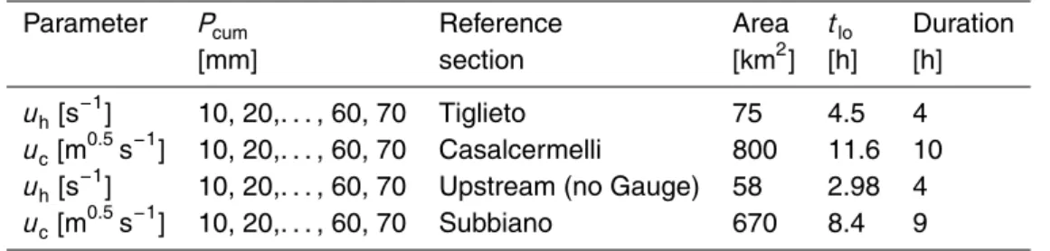
The estimation of the overland and channel flow parameters was carried out by using geomorphological information derived from the DEM. The methodology is described in Silvestro et al. (2013), and we synthetically report its description in the following paragraphs and in Fig. 9:

(18)

HESSD

Step 1. Identify a formulation to estimate the typical lag time (t_lo: temporal distance between the centre of mass of the hydrograph and the centre of mass of the mean hyetograph) of a basin based on its main morphologic characteristics. The soil was considered to be completely impermeable so that the subsurface and deep flow parameters (c_t,c_f,R_f and Vw_max) therefore become irrelevant.

5

Step 2. Identify two sections along the streamline of the basin, one at the head of

the basin and the other downstream. Estimate the lag-time,t_lobased on the DEM

and geographical information.

Step 3. Generate a set of synthetic events with constant intensity in space and in timehaving duration equal to the typical response time of the basin closed at the

10

sections (see an example in Table 3).

Step 4. Set a first estimate for the value of u_c and calibrate u_h for each value of

P_cumreferring to the upstream section, using the objective function to minimize:

Of =|t_lo−t_lm| (10)

15

Wheret_lois thet_lderived by the geomorphologic characteristics of the basin while

t_lmis the t_lobtained from the model simulations. Calculate the average of theu_h

values.

Step 5. Fixu_h and calibrate u_c as in Steps 3 and 4, but referring instead to the

downstream section.

20

Step 6. Iterate the process until it converges.

According to Silvestro et al. (2013), it is possible to separate the calibration of the two surface flow parameters. In the case of head sections with reduced paths in

channelized networks, the influence of u_c is scarce; as a consequence, an average

value ofu_c can be set and the calibration can be done only for u_v. The value of u_c is

(19)

HESSD

then calibrated based on data from a downstream section with a longer channelized network. This procedure is iterated as shown in Fig. 9. Usually 3–4 iterations are sufficient for a good convergence of the process.

5.2.2 Subsurface parameters (ctandcf) – exploiting LST and SWI satellite

estimate

5

Once the surface flow parameters are estimated, the subsurface soil parameters can be evaluated optimizing a proper score between satellite derived and modelled LST (Silvestro et al., 2013) or SWI. In this case we considered the Bias and Nash–Sutcliffe at basin scale for LST for SWI as statistics.

6 Results: calibration and verification on multi-yearly simulations

10

6.1 Orba basin

The calibration with the multi-objective function was carried out considering the period July–October 2009 for LST comparison, July–November 2011 for SWI comparison and August–October 2006 for streamflow comparison. In the second period, two intense events preceded by periods of droughts occurred; as a result, the model is forced to

15

work under extreme conditions. The streamflow threshold used in the third component of the M.O. function isQ_T=200 m3s−1.

The calibration using streamflow data only (here after S.N.) was also considered in order to compare the results of M.O. and R.S. approaches with standard calibration strategies. The R.S. approaches using LST or SWI will be indicated R.S.(LST)

20

and R.S.(SWI) respectively hereafter. The maximization of Nash–Sutcliffe coefficient

between modeled and observed streamflow is used.

The parameter sets obtained by the three calibration strategies are reported in Table 4.

(20)

HESSD

The surface flow parameters obtained with the R.S. and M.O. calibration

methodologies are similar, while the S.N. method produces higher u_c and lower u_h

values. In the case of sub-surface flow, the values are a little bit different for the three

considered cases probably because they are more sensitive to the different adopted

approaches (Efstratiadis and Koutsoyiannis, 2010).

5

Figure 10 reports values of the Nash–Sutcliffe coefficient (that depends only on the streamflow) vs. values of the objective function of the M.O. approach. Hydrographs derived from the parameter sets having the best values of S.N. and M.O are shown. The parameter values that optimize the single score (NS) are not the same that optimize the M.O. function.

10

Obviously, the choice of the single components of the M.O. function influences the way the various variables impact on the final results, but the applied methodology proposed by Madsen (2000) helps to normalize and balance the weights of the components.

Validation of multi-annual simulations were carried out using the parameters

15

calibrated with the proposed methodologies. The validation period is from 1 January 2006 to 31 December 2011; the first five months were used for the model warm up.

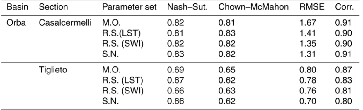
In Table 5, the score values are reported while Figs. 11 and 12 show the main events. In each figure some significant sub-periods are reported while in the bottom panel the

20

entire simulation period using a logarithmic scale is shown.

The values of the scores are good in all the cases. The Casalcermelli section performances are better than those for Tiglieto, this may be due to the fact that the first section corresponds to a larger drainage area and therefore the integration effects smooth the uncertainties of the rainfall fields. The M.O. approach leads to score values

25

on the streamflow similar to the S.N. method in the validation period, while the R.S. approach produced poorer performance with respect to the other two approaches. Notwithstanding, all the parameters sets led to good results in terms of the modelled hydrographs.

(21)

HESSD

The M.O. calibration strategy lead to good performances in reproducing the observed streamflows despite the fact that these latter measurements are not the only ones used in the calibration process; there are good performances over long periods of simulation for both of the considered outlet sections. The peak flows and the time of the peak flows are generally well reproduced as well as the periods of flow recession and drought

5

between the most relevant events.

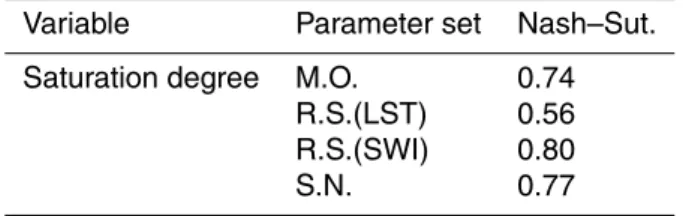
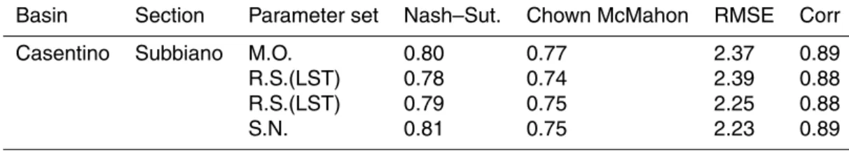
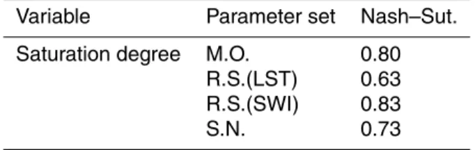
The series of mean LST at basin scale were compared with LST satellite estimation. A similar comparison was made between the satellite SWI and modelled saturation degree. Tables 6 and 7 show the values of the scores for the three considered parameters sets.

10

The classic calibration obtained with the maximization of the Nash Sutcliffe

coefficient of the streamflow (S.N.) allows for obtaining good performances in terms

of streamflow simulation, but it produces higher values of LST bias, while the M.O.

approaches balance between the different components. The reproduction of SWI is

quite good for both the M.O. and S.N. cases.

15

The accumulated discharge volume simulated by the model was compared with that derived from the streamflow observations in order to verify the behavior of the model in terms of total runoffvolumes. The results are reported in Fig. 13. The model reproduced with fine approximation the observed volumes; the error on the entire period is

approximately−1.9,−1.3,−3.0, and−2.5 % for M.O, R.S.(LST), R.S.(SWI) and S.N.,

20

respectively. These errors are probably lower than the uncertainties introduced by the level-discharge transformation.

6.2 Casentino basin

The calibration with the multi-objective function was carried out considering the period July–November 2009 for LST comparison, August–November 2009 for SWI

25

comparison and September–December 2005 for streamflow comparison. The periods

(22)

HESSD

streamflow threshold used in the third component of the M.O. function was Q_T=

200 m3s−1. The parameter sets are reported in Table 8.

In Table 9 the scores are reported, while Figs. 14 and 15 show the main discharge

events. The figures report different significant events, while in the bottom panel the

entire simulation period is shown using a logarithmic scale.

5

Tables 10 and 11 show the values of the scores for the variables LST and S.H. The values of the scores are good in all the cases; they are better for M.O. with respect to S.N. for both LST and Saturation Degree variables.

The model furnishes good performances over long periods for all the three

considered calibration strategies; the M.O. calibration method allows good

10

performances in reproducing streamflow observations (the results are better than the Orba basin).

The accumulated volume over the 7 years of simulation is generally well simulated (Fig. 16); in this case, there is a larger difference between the total volumes obtained with the two different parameter sets, the errors are in fact of the order of 9, 8.8, 5.3,

15

and 4 % for M.O., R.S.(LST), R.S.(SWI) and N.S., respectively. The errors on the total volume are a little larger than the case of Orba basin.

7 Discussion and conclusions

This paper shows that satellite data are useful in reducing the uncertainty of the parameterization of a distributed hydrological model and that they can be used in

20

calibration strategy to improve model representation of hydrological processes.

The model used is Continuum (Silvestro et al., 2013), which simulates LST and Soil Moisture as state variables. Two Italian basins were considered and validation over extended periods was realized.

The uncertainty analysis (Zappa et al., 2010; Shen et al., 2012) of the most sensitive

25

parameters shows that the equifinality can be reduced using Land Surface Temperature and Soil Water Index satellite estimations.

(23)

HESSD

Two methodologies to estimate a subset of the parameters of the model by exploiting remote sensing were applied. The first methodology consists of the minimization of a multi-objective function that depends on streamflow, LST and Soil Moisture. The second methodology simulates the case when no streamflow data are available and the calibration is carried out based only on LST satellite data and information derived

5

from a DEM.

A multi-year period validation was done in terms of reproduction of both streamflow time series and total volume over the considered period. A comparison with a standard calibration strategy based on streamflow data was also carried out.

The results are encouraging, the skill scores show good performance and, even if the

10

observed and simulated streamflow are in some cases quite different, the general trend

is good and there are not large biases in terms of runoffvolumes over long simulation

periods. The largest errors seem to be more related to the uncertainties of the input rainfall fields rather than on the model parameterization. Moreover, the errors on LST and Saturation Degree are generally lower in the case of parameter sets derived by

15

the multi objective approach with respect to those obtained by the streamflow based calibration strategy.

Both the results of calibration and uncertainty analysis confirm that a way to reduce equifinality and to augment the parameter constraints is related to the increasing of model state and output variables that can be derived from both gauge and remote

20

sensing data. This helps to reduce the possibility of obtaining similar results with a large number of parameter sets.

In addition, remote sensing data (in this specific case the LST and Soil Moisture) offer alternative ways to carry out parameter calibration in cases where no streamflow data might be available. Satellite derived data such as DEM and LST are generally

25

universally available.

We can thus state that the presented work successfully explored the direction proposed by Seibert and McDonnel (2002) and Efstratiadis and KoutsoYiannis (2010),

(24)

HESSD

which consisted of obtaining a better overall performance of the model and ensure consistency across its various aspects.

The described methodologies can be adapted and applied to other hydrological models that have characteristics similar to Continuum and that can simulate LST and soil moisture as state variables; moreover, these methods can be extended by referring

5

to other remote sensing data, and in general observed data, that can be reproduced by the model. More the model has the capability of reproducing observable quantities (e.g. evapotranspiration, soil humidity, etc.) more constraints can be to imposed to the model can increase.

The results of the presented work can be read from two different points of view.

10

On one hand, it highlights the advantages of using distributed hydrological models that allow for the reproducing with some degree of detail the physical processes, such models in fact, simulate a larger number of variables which can also be observed. On the other hand, it highlights the opportunities given by remote sensing and the necessity of augmenting the number (and the quality) of these data. Remotely sense

15

data can in fact be used to parameterize hydrological models and to set up constraints to the parameters in the calibration process.

Acknowledgements. This work is supported by the Italian Civil Protection Department, and by the Italian Regions of Valle d’Aosta and Liguria. We acknowledge the Italian Civil Protection Department for providing us with the data from the regional meteorological observation

20

networks. We also thank the H-SAF project for the availability of Surface Soil Moisture data.

References

Albergel, C., Rüdiger, C., Pellarin, T., Calvet, J.-C., Fritz, N., Froissard, F., Suquia, D., Petitpa, A., Piguet, B., and Martin, E.: From near-surface to root-zone soil moisture using an exponential filter: an assessment of the method based on in situ observations and model simulations,

25

Hydrol. Earth Syst. Sci., 12, 1323–1337, doi:10.5194/hess-12-1323-2008, 2008.

Albergel, C., de Rosnay, P., Gruhierand, C., Munoz-Sabater, J., Hasenauer, S., Isaksen, L., Kerr, Y., and Wagner, W.: Evaluation of remotely sensed and modelled soil moisture products

(25)

HESSD

using global ground-based in situ observations, Remote Sens. Environ., 118, 215–226, 2012.

Bartalis, Z., Wagner, W., Naeimi, V., Hasenauer, S., Scipal, K., Bonekamp, H. Figa, J. C., and Anderson, C.: Initial soil moisture retrievals from the METOP-A advanced scatterometer (ASCAT), Geophys. Res. Lett., 34, L20401, doi:10.1029/2007GL031088, 2007.

5

Beven, K. and Binley, A. M.: The future of distributed models: model calibration and uncertainty prediction, Hydrol. Proc., 24, 43–69, 1992.

Bitew, M. M. and Gebremichael, M.: Evaluation of satellite rainfall products through hydrologic simulation in a fully distributed hydrologic model, Water Resour. Res., 47, W06526, doi:10.1029/2010WR009917, 2011.

10

Bjerklie, D. M., Dingman, S. L., Vorosmarty, C. J., Bolster, C. H., and Congalton, R. G.: Evaluating the potential for measuring river discharge from space, J. Hydrol., 278, 17–38, 2003.

Brakenridge, G. R., Nghiem, S. V., Anderson, E. A., and Chien, S.: Space-based measurement of river runoff, EOS T. Am. Geophys. Un., 86, 185–188, doi:10.1029/2005EO190001, 2005.

15

Brakenridge, G. R., Cohen, S., Kettner, A. J., De Groeve, T., Nghiem, S. V., Syvitski, J. P., and Fekete, B. M.: Calibration of satellite measurements of river discharge using a global hydrology model, J. Hydrol., 475, 123–136, 2012.

Brocca, L., Melone, F., Moramarco, T., Wagner, W., and Hasenauer, S.: ASCAT soil wetness index validation through in situ and modelled soil moisture data in central Italy, Remote Sens.

20

Environ., 114, 2745–2755, doi:10.1016/j.rse.2010.06.009, 2010.

Brocca, L., Hasenauer, S., Lacava, T., Melone, F., Moramarco, T., Wagner, W., Dorigo, W., Matgen, P., Martínez-Fernández, J., Llorens, P., Latron, J., Martin, C., and Bittelli, M.: Soil moisture estimation through ASCAT and AMSR-E sensors: an intercomparison and validation study across Europe, Remote Sens. Environ.,115, 3390–3408, 2011a.

25

Brocca, L., Melone, F., and Moramarco, T.: Distributed rainfall–runoff modelling for flood frequency estimation and flood forecasting, Hydrol. Process., 25, 2801–2813, 2011b. Caparrini, F., Castelli, F., and Entekhabi, D.: Estimation of surface turbulent fluxes through

assimilation of radiometric surface temperature sequences, J. Hydrometeorol., 5, 145–159, 2004.

30

Carpenter, T. M. and Georgakakos, K. P.: Intercomparison of lumped versus distributed hydrologic model ensemble simulations on operational forecast scales, J. Hydrol., 329, 174– 185, 2006.

(26)

HESSD

Coccia, G., Mazzetti, C., Ortiz, E. A., and Todini, E.. Application of the Topkapi model within the DMIP 2 project, Paper 4.2, in: 23rd Conference on Hydrology, 89th Meeting of the AMS, Phoenix, Arizona, 10–16 January 2009, https://ams.confex.com/ams/pdfpapers/149632.pdf, last last access: 6 June 2014, 2009.

Crow, W. T., Berg, A. A., Cosh, M. H., Loew, A., Mohanty, B. P., Panciera, R., de Rosnay, P.,

5

Ryu, D., and Walker, J. P.: Upscaling sparse groundbased soil moisture observations for the validation of coarseresolution satellite soil moisture products, Rev. Geophys., 50, RG2002, doi:10.1029/2011RG000372, 2012.

Chiew, F. and McMahon, T.: Application of the daily rainfall–runoffmodel MODHYDROLOG to 28 Australian catchments, J. Hydrol., 153, 383–416, 1994.

10

Dickinson, R.: The force-restore method for surface temperature and its generalization, J. Climate, 1, 1086–1097, 1988.

Efstratiadis, A. and Koustoyiannis, D.: One decade of Multi-Objective calibration approaches in hydrological modelling: a review, Hydrol. Sci. J., 55, 58–78, 2010.

EUMETSAT: Product user manual, vegetation parameters, available at: http://landsaf.meteo.pt/,

15

last access: 10 March 2011, 2008.

EUMETSAT: Algorithm theoretical Basis Document for Land Surface Temperature (LST), available at: http://landsaf.meteo.pt/, last access: 22 September 2011, 2009.

Flores, A. N., Entekhabi, D., and Bras, R. L.: Reproducibility of soil moisture ensembles when representing soil parameter uncertainty using a Latin Hypercube–based approach with

20

correlation control, Water Resour. Res., 46, W04506, doi:10.1029/2009WR008155, 2010. Gabellani, S., Silvestro, F., Rudari, R., and Boni, G.: General calibration methodology for

a combined Horton-SCS infiltration scheme in flash flood modeling, Nat. Hazards Earth Sci., 8, 1317–1327, 2008.

Giannoni, F., Roth, G., and Rudari, R.: A semi – distributed rainfall–runoff model based on

25

a geomorphologic approach, Phys. Chem. Earth, 25, 665–671, 2000.

Giannoni, F., Roth, G., and Rudari, R.: A procedure for drainage network identification from geomorphology and its application to the prediction of the hydrologic response, Adv. Water Resour., 28, 6, 567–581, 2005.

Göttsche, F. M. and Hulley, G. C.: Validation of six satellite-retrieved land surface emissivity

30

products over two land cover types in a hyper-arid region, Remote Sens. Environ., 124, 149– 158, 2012.

(27)

HESSD

Khan, S. I., Hong, Y., Wang, J., Yilmaz, K. K., Gourley, J. J., Adler, R. F., Brakenridge, G. R., Policelli, F., Habib, S., and Irwin, D.: Satellite remote sensing and hydrologic modeling for flood inundation mapping in Lake Victoria Basin: implications for hydrologic prediction in ungauged basins, IEEE T. Geosci. Remote, 49, 85–95, 2011.

Koren, V., Moreda, F., and Smith, M.: Use of soil moisture observations to improve parameter

5

consistency, J. Phys. Chem. Earth, 33, 1068–1080, doi:10.1016/j.pce.2008.01.003, 2008. Kim, S. M., Benham, B. L., Brannan, K. M., Zeckoski, R. W., and Doherty, J.: Comparison of

hydrologic calibration of HSPF using automatic and manual methods, Water Resour. Res., 43, W01402, doi:10.1029/2006WR004883, 2007.

Kunstmann, H., Krause, J., and Mayr, S.: Inverse distributed hydrological modelling of Alpine

10

catchments, Hydrol. Earth Syst. Sci., 10, 395–412, doi:10.5194/hess-10-395-2006, 2006. Lin, J. D.: On the Force-Restore method for prediction of ground surface temperature, J.

Geophys. Res., 85, 3251–3254, 1980.

Liu., Z., Martina, M. L. V., and Todini, E.: Flood forecasting using a fully distributed model: application of the TOPKAPI model to Upper Xixian Catchment, Hydrol. Earth Syst. Sci., 9,

15

347–364, 2005,

http://www.hydrol-earth-syst-sci.net/9/347/2005/.

Madsen, H.: Automatic calibration of a conceptual rainfall–runoff model using multiple objectives, J. Hydrol., 235, 276–288, 2000.

Madsen, H.: Parameter estimation in distributed hydrological catchment modelling using

20

automatic calibration with multiple objectives, Adv. Water Resour., 26, 205–216, 2003. Maidment, D.: Handbook of Hydrology, McGraw-Hill, Inc., USA, 1992.

Montaldo, N., Rondena, R., Albertson, J. D., and Mancini. M.: Parsimonious modelling of vegetation dynamics for ecohydrological studies of waterlimited ecosystems, Water Resour. Res., 41, W10416, doi:10.1029/2005WR004094, 2005.

25

Murray, S. J., Watson, I. M., and Prentice, I. C.: The use of dynamic global vegetation models for simulating hydrology and the potential integration of satellite observations, Prog. Phys. Geogr., 37, 63–97, doi:10.1177/0309133312460072, 2013.

Naeimi, V., Scipal, K., Bartalis, Z., Hasenauer, S., and Wagner, W.: An improved soil moisture retrieval algorithm for ERS and METOP scatterometer observations, IEEE T. Geosci.

30

Remote, 47, 1999–2013, 2009.

Nash, J. E. and Sutcliffe, J. V: River flood forecasting through conceptual models I: a discussion of principles, J. Hydrol., 10, 282–290, 1970.

(28)

HESSD

Pavelsky, T. M.: Using widthbased rating curves from spatially discontinuous satellite imagery to monitor river discharge, Hydrol. Process., 28, 3035–3040, 2014.

Perrin, C., Michel, C., and Andréassian, V.: Does a large number of parameters enhance model performance? Comparative assessment of common catchment model structures on 429 catchments, J. Hydrol., 242, 275–301, 2001.

5

Ridler, M. E., Sandholt, I., Butts, M., Lerer, S., Mougin, E., Timouk, F., Kergoat, L., and Madsen, E.: Calibrating a soil–vegetation–atmosphere transfer model with remote sensing estimates of surface temperature and soil surface moisture in a semi arid environment, J. Hydrol., 436–437, 1–12, 2012.

Rhoads, J., Dubayah, R., Lettenmaier, D., O’Donnell, G., and Lakshmi, V.: Validation of land

10

surface models using satellite derived surface temperature, J. Geophys. Res., 106, 20085– 20099, 2001.

Savenije, H. H. G.: Equifinality, a blessing in disguise?, Hydrol. Proc., 15, 2835–2838, 2001. Schmugge, T. J., Kustas, W. P., Ritchie, J. C., Jackson, T. J., and Rango, A.: Remote sensing in

hydrology, Adv. Water Resour., 25, 1367–1385, 2002.

15

Shen, Z. Y., Chen, L., and Chen, T.: Analysis of parameter uncertainty in hydrological and sediment modeling using GLUE method: a case study of SWAT model applied to Three Gorges Reservoir Region, China, Hydrol. Earth Syst. Sci., 16, 121–132, doi:10.5194/hess-16-121-2012, 2012.

Silvestro, F., Gabellani, S., Delogu, F., Rudari, R., and Boni, G.: Exploiting remote sensing land

20

surface temperature in distributed hydrological modelling: the example of the Continuum model, Hydrol. Earth Syst. Sci., 17, 39–62, doi:10.5194/hess-17-39-2013, 2013.

Singh, S. K. and Bárdossy, A.: Calibration of hydrological models on hydrologically unusual events, Adv. Water Resour., 38, 81–91, doi:10.1016/j.advwatres.2011.12.006, 2012.

Sini, F., Boni, G., Caparrini, F., and Entekhabi, D.: Estimation of largescale evaporation fields

25

based on assimilation of remotely sensed land temperature, Water Resour. Res., 44, W06410, doi:10.1029/2006WR005574, 2008.

Stroud, P. D.: A recursive exponential filter for time-sensitive data, Los Alamos national Laboratory, LAUR-99-5573, available at: public.lanl.gov/stroud/ExpFilter/ExpFilter995573. pdf, last access: July 2008, 1999.

30

Todini, E.: History and perspective of hydrological catchment modelling, in: Water, Environment, Energy and Society, edited by: Jain, S. K., Singh, V. P., Kumar, V., Kumar, R., Singh, R. D.,

(29)

HESSD

Sharma, K. D., Proc. Of WEES-2009, Allied Publishers Pvt. Ltd, New Delhi (India), 512–523, 2009.

Todini, E. and Ciarapica, L.: The TOPKAPI model. Mathematical models of large watershed hydrology, in: Water Resources Publications, edited by: Singh, V. P. and Frevert, D. K., Littleton, Colorado, ch. 12, 471–506, 2002.

5

Vörösmarty, C., Askew, A., Grabs, W., Barry, R. G., Birkett, C., Döll, P., Goodison, B., Hall, A., Jenne, R., Kitaev, L., Landwehr, J., Keeler, M., Leavesley, G., Schaake, J., Strzepek, K., Sundarvel, S. S., Takeuch, K., and Webster, F.: Global water data: a newly endangered species, EOS T. Am. Geophys. Un., 82, 54–58, 2001.

Vrugt, J. A., Gupta, H. V., Bouten, W. and Sorooshian, S.: A shuffled complex evolution

10

metropolis algorithm for optimization and uncertainty assessment of hydrologic model parameters, Water Resour. Res., 39, 1201, doi:10.1029/2002WR001642,

Wagner, W., Lemoine, G., and Rott, H.: A method for estimating soil moisture from ERS scatterometer and soil data, Remote Sens. Environ., 70, 191–207, 1999.

Wagner, W., Hahn, S., Kidd, R., Melzer, T., Bartalis, Z., Hasenauer, S., Figa, J., de

15

Rosnay, P., Jann, A., Schneider, S., Komma, J., Kubu, G., Brugger, K., Aubrecht, C., Zuger, J., Gangkofner, U., Kienberger, S., Brocca, L., Wang, Y., Bloeschl, G., Eitzinger, J., Steinnocher, K., Zeil, P., and Rubel, F.: The ASCAT soil moisture product: specifications, validation results, and emerging applications, Meteorol. Z., 22, 5–33, doi:10.1127/0941-2948/2013/0399, 2013.

20

Ward, A. D. and Trimble, W.: Environmental Hydrology, 2nd Edn., CRC Press, USA, 504 pp., December 2003.

White, C. D. and Lewis, M. M.: A new approach to monitoring spatial distribution and dynamics of wetlands and associated flows of Australian Great Artesian Basin springs using QuickBird satellite imagery, J. Hydrol., 408, 140–152, 2011.

25

Wooding, R. A.: A hydraulic modeling of the catchment-stream problem, 1. Kinematic wave theory, J. Hydrol., 3, 254–267, 1965.

Xu, D., Wang, W., Chau, K., Cheng, C., and Chen, S.: Comparison of three global optimization algorithms for calibration of the Xinanjiang model parameters, J. Hydroinform., 15.1, 174– 193, 2013.

30

Yapo, P. O., Gupta, H. V., and Sorooshian, S.: Multi-Objective global optimization for hydrological models, J. Hydrol., 204, 83–97, 1998.