Markowitz Minimum Variance Portfolio Optimization
using New Machine Learning Methods
by
Oluwatoyin Abimbola Awoye
Thesis
submitted in partial fulfillment of the requirements for the degree of
Doctor of Philosophy in Computer Science
Department of Computer Science University College London
Gower Street United Kingdom Email: [email protected]
ii
Declaration
iii
Acknowledgements
iv
Abstract
v
List of Figures
xiv
List of Tables
xvii
List of Abbreviations
xxi
iii
Declaration
I, Oluwatoyin Awoye, confirm that the work presented here is my own. When results have been derived from other sources this is indicated in the text.
iv
Acknowledgements
First and foremost, I would like to thank God for continual guidance during this research. I would like to thank my main supervisor, Prof. John Shawe-Taylor for allowing me to undergo this research under his guidance. I would like to thank him for all his invaluable advice, pushing me and especially pointing me in the right direction to have contact with other researchers who have been beneficial to me.
I would like to thank Dr. Mark Herbster, who acted as my second supervisor. Mark has done more than is typical for that role, being extremely generous with his time especially during the early years of my research and I have benefited immensely from this. I would also like to thank Dr. Zakria Hussain, who directed me towards the required background on Markowitz portfolio optimization and its application in industry. I am grateful to my colleagues at the UCL Computer Science department for providing a supporting research atmosphere.
I would also like to thank my family for their encouragement throughout my research experience. To my husband, Yinka, thank you for being a great example to me, for your constant love, support and motivation throughout the years. Lastly, I would like to thank my parents for supporting and providing me with the necessary funding to undertake this research work. I am forever grateful and to them I dedicate this thesis.
v
Abstract
The use of improved covariance matrix estimators as an alternative to the sample covariance is considered an important approach for enhancing portfolio optimization. In this thesis, we propose the use of sparse inverse covariance estimation for Markowitz minimum variance portfolio optimization, using existing methodology known as Graphical Lasso [16], which is an algorithm used to estimate the inverse covariance matrix from observations from a multivariate Gaussian distribution.
We begin by benchmarking Graphical Lasso, showing the importance of regularization to control sparsity. Experimental results show that Graphical Lasso has a tendency to overestimate the diagonal elements of the estimated inverse covariance matrix as the regularization increases. To remedy this, we introduce a new method of setting the optimal regularization which shows performance that is at least as good as the original method by [16].
Next, we show the application of Graphical Lasso in a bioinformatics gene microarray tissue classification problem where we have a large number of genes relative to the number of samples. We perform dimensionality reduction by estimating graphical Gaussian models using Graphical Lasso, and using gene group average expression levels as opposed to individual expression levels to classify samples. We compare classification performance with the sample covariance, and show that the sample covariance performs better.
Finally, we use Graphical Lasso in combination with validation techniques that optimize portfolio criteria (risk, return etc.) and Gaussian likelihood to generate
vi
new portfolio strategies to be used for portfolio optimization with and without short selling constraints. We compare performance on synthetic and real stock market data with existing covariance estimators in literature, and show that the newly developed portfolio strategies perform well, although performance of all methods depend on the ratio between the estimation period and number of stocks, and on the presence or absence of short selling constraints.
vii
Contents
1
Introduction
1
1.1 Background ... 1 1.2 Motivation... 2 1.3 Contribution ... 31.4 The Organization of the Thesis ... 5
PART I: Benchmarking the Graphical Lasso
2
Evaluation of the Graphical Lasso Algorithm
8
2.1 Introduction to the Sparse Inverse Covariance ... 82.2 Undirected Graphical Models ... 10
2.2.1 Graphical Gaussian Model ... 12
2.2.2 The Benefits of Sparsity ... 13
2.2.3 Inexact Methods for the Inverse Covariance Estimation .. 14
2.2.3.1 Covariance Selection Discrete Optimization ... 14
2.2.3.2 Neighborhood Selection with the Lasso ... 15
2.2.4 Exact Methods for the Inverse Covariance Estimation ... 17
2.2.4.1 L1-penalised Methods ... 17
2.3 Introduction to the Graphical Lasso ... 19
viii
Contents
2.3.2 A Method for Penalty Selection ... 24
2.4 A New Method for Penalty Selection ... 26
2.4.1 The Model ... 26
2.4.2 Generating Synthetic Data ... 28
2.4.3 Performance Measure ... 29
2.5 Experiment Results ... 30
2.5.1 Model 1 Results ... 30
2.5.2 Model 2 Results ... 36
2.6 Summary ... 41
3
Graphical Lasso Application to Bioinformatics
43
3.1 Introduction ... 443.1.1 DNA Microarray Data Characteristics ... 47
3.1.1.1 The Curse of Dimensionality ... 47
3.1.1.2 Noise and Data Normalization ... 47
3.2 Graphical Models and Gene Microarray Data ... 48
3.3 Microarray Data Analysis using Graphical Lasso ... 51
3.3.1 The Data ... 52
3.3.2 Microarray Classification Problem Definition ... 54
3.3.3 The Proposed Method ... 55
3.3.4 Data Pre-processing: Centering the Data ... 55
ix
Contents
3.3.6 k-Nearest Neighbor Graphs to Visualize Interaction ... 60
3.3.7 Supervised Learning Methodology ... 64
3.3.7.1 Linear Least Squares Regression Classifier ... 65
3.3.7.2 Ridge Regression Classifier ... 66
3.4 Two-class Classification to Identify Tissue Samples ... 67
3.4.1 Methodology ... 67
3.4.2 Linear Least Squares Regression Classification Results ... 68
3.4.3 Ridge Regression Classification Results ... 70
3.5 One-versus-all Classification to Identify Tissue Samples ... 72
3.5.1 Methodology ... 73
3.5.2 Linear Least Squares Regression Classification Results ... 73
3.5.3 Ridge Regression Classification Results ... 75
3.6 Using Random Genes to Identify Tissue Samples ... 76
3.6.1 Two-class Classification to Identify Tissue Samples... 77
3.6.1.1 Ridge Regression Classification Results ... 77
3.6.2 One-versus-all Classification to Identify Tissue Samples . 79 3.6.2.1 Ridge Regression Classification Results ... 79
x
Contents
PART II: Graphical Lasso Application to Finance
4
Graphical Lasso and Portfolio Optimization
85
4.1 Markowitz Mean-Variance Model ... 85
4.2 Efficient Frontier ... 86
4.2.1 Mathematical Notations ... 87
4.3 Linear Constraints ... 91
4.4 Global Minimum-Variance Portfolio Optimization ... 93
4.5 Limitations of the Markowitz Approach ... 95
4.6 Synthetic Data Experiment ... 96
4.6.1 Generating Synthetic Data ... 97
4.6.2 Methodology ... 98
4.6.3 Graphical Lasso Portfolio Strategies ...101
4.6.4 Performance Measures ...103 4.6.4.1 Predicted Risk ...103 4.6.4.2 Realized Risk ...103 4.6.4.3 Empirical Risk ...104 4.6.4.4 Realized Likelihood ...104 4.6.4.5 Empirical Likelihood ...104
4.6.4.6 Sparsity Level and Zero-overlap ...105
4.7 Experiment Results ... 105
xi
Contents
4.7.1.1 Realized Risk ...106
4.7.1.2 Empirical Risk ...109
4.7.1.3 Empirical and Realized Likelihood ...110
4.7.1.4 Portfolio Measures Correlation Analysis ...112
4.7.2 Long-only Portfolio Results ...114
4.7.2.1 Realized Risk ...115
4.7.2.2 Empirical Risk ...117
4.7.2.3 Empirical and Realized Likelihood ...119
4.7.2.4 Portfolio Measures Correlation Analysis ...121
4.8 Summary ... 122
5
Covariance Estimation and Portfolio Optimization: A
Comparison between Existing Methods and the New Sparse
Inverse Covariance Method 125
5.1 Covariance and Mean-Variance Portfolio Optimization ...125
5.2 Covariance Estimation: Existing Methods ...126
5.2.1 Direct Optimization ... 126
5.2.2 Spectral Estimators ... 127
5.2.2.1 The Single Index Model ... 127
5.2.2.2 Random Matrix Theory Models ...127
xii
Contents
5.2.3.1 Shrinkage to Single Index ... 131
5.2.3.2 Shrinkage to Common Covariance ... 131
5.2.3.3 Shrinkage to Constant Correlation ... 132
5.3 Experiment on Stock Market Data ... 132
5.3.1 Data ... 133
5.3.2 Methodology ...133
5.3.3 Performance Measures ...135
5.3.3.1 Sharpe ratio ...135
5.4 Experiment Results ... 136
5.4.1 Long-short Portfolio Results ... 136
5.4.1.1 Realized Risk ...137
5.4.1.2 Expected Return of the Portfolio ...141
5.4.1.3 Sharpe ratio ...145
5.4.2 Long-only Portfolio Results ...148
5.4.2.1 Realized Risk ...148
5.4.2.2 Expected Return of the Portfolio ...152
5.4.2.3 Sharpe ratio ...154
5.5 Summary ... 157
6
Conclusion and Future work
160
6.1 Conclusion ... 160xiii
Appendices
166
xiv
List of Figures
Fig. 2.1 Example of a sparse undirected graph... 11
Fig. 2.2 Example of an undirected graphical model ... 11
Fig. 2.3 Original sparse precision versus Graphical Lasso solution (ρ=0.1) ... 21
Fig. 2.4 Original sparse precision versus Graphical Lasso solution (ρ=0.4) ... 22
Fig. 2.5 Original sparse precision versus Graphical Lasso solution (ρ=1) ... 23
Fig. 2.6 Original sparse precision versus Graphical Lasso solution (ρ=2) ... 23
Fig. 2.7 Model 1 error between Graphical Lasso and Modified Graphical Lasso (p=10) ... 30
Fig. 2.8 Model 1 optimal penalty for Graphical Lasso and Modified Graphical Lasso (p=10) ... 30
Fig. 2.9 Model 1 error between Graphical Lasso and Modified Graphical Lasso (p=30) ... 31
Fig. 2.10 Model 1 optimal penalty for Graphical Lasso and Modified Graphical Lasso (p=30) ... 32
Fig. 2.11 Model 1 error between Graphical Lasso and Modified Graphical Lasso (p=50) ... 32
Fig. 2.12 Model 1 optimal penalty for Graphical Lasso and Modified Graphical Lasso (p=50) ... 33
Fig. 2.13 Model 1 error between Graphical Lasso and Modified Graphical Lasso (p=70) ... 34
Fig. 2.14 Model 1 optimal penalty for Graphical Lasso and Modified Graphical Lasso (p=70) ... 34
xv
List of Figures
Fig. 2.15 Model 2 error between Graphical Lasso and Modified Graphical Lasso
(p=10) ... 36
Fig. 2.16 Model 2 optimal penalty for Graphical Lasso and Modified Graphical Lasso (p=10) ... 36
Fig. 2.17 Model 2 error between Graphical Lasso and Modified Graphical Lasso (p=30) ... 37
Fig. 2.18 Model 2 optimal penalty for Graphical Lasso and Modified Graphical Lasso (p=30) ... 38
Fig. 2.19 Model 2 error between Graphical Lasso and Modified Graphical Lasso (p=50) ... 38
Fig. 2.20 Model 2 optimal penalty for Graphical Lasso and Modified Graphical Lasso (p=50) ... 39
Fig. 2.21 Model 2 error between Graphical Lasso and Modified Graphical Lasso (p=70) ... 40
Fig. 2.22 Model 2 optimal penalty for Graphical Lasso and Modified Graphical Lasso (p=70) ... 40
Fig. 3.1 DNA microarray image ... 44
Fig. 3.2 Acquiring the gene expression data from DNA microarray ... 45
Fig. 3.3 The distribution of the microarray data samples before centering ... 57
Fig. 3.4 The distribution of the microarray data samples after centering ... 57
xvi
List of Figures
Fig. 3.6 Sparsity of estimated Precision (ρ=3) ... 59
Fig. 3.7 Sparsity of estimated Precision (ρ=10) ... 59
Fig. 3.8 Covariance k-NN graph – 3 total sub-networks ... 62
Fig. 3.9 Precision (ρ=1) k-NN graph – 20 total sub-networks ... 63
Fig. 3.10 Precision (ρ=3) k-NN graph – 14 total sub-networks ... 64
Fig. 4.1 The efficient frontier ... 91
xvii
List of Tables
Table 3.1 Tissue types and the distribution of the 255 tissue samples ... 54
Table 3.2 Structure of the Precision as regularization ρ is increased ... 60
Table 3.3 LLS two-class average classification results ... 68
Table 3.4 LLS two-class covariance classification results ... 69
Table 3.5 LLS two-class precision (ρ=1) classification Results ... 69
Table 3.6 LLS two-class precision (ρ=3) classification Results ... 70
Table 3.7 Ridge regression two-class average classification results ... 70
Table 3.8 Ridge regression two-class covariance classification results ... 71
Table 3.9 Ridge regression two-class precision (ρ=1) classification results ... 71
Table 3.10 Ridge regression two-class precision (ρ=3) classification results ... 72
Table 3.11 LLS one-versus-all average classification results ... 74
Table 3.12 LLS one-versus-all classification results ... 74
Table 3.13 Ridge regression one-versus-all average classification results ... 75
Table 3.14 Ridge regression one-versus-all classification results ... 76
Table 3.15 Two-class average classification results for the precision and covariance classifiers with random gene replacement ... 78
Table 3.16 Ridge regression two-class average classification results for the precision and covariance classifiers without random gene replacement ... 78
Table 3.17 Ridge regression one-versus-all average classification results for the precision and covariance classifiers with Random gene replacement ... 79
Table 3.18 Ridge regression one-versus-all average classification results for the precision and covariance classifiers without random gene replacement ... 79
xviii
List of Tables
Table 3.19 Ridge regression one-versus-all classification results for the
covariance classifier with and without random gene replacement ... 81
Table 3.20 Ridge regression one-versus-all classification results for precision (ρ=1) with and without random gene replacement ... 81
Table 3.21 Ridge regression one versus all classification results for precision (ρ=3) with and without random gene replacement ... 82
Table 4.1 Long-short portfolio average realized risks ...106
Table 4.2 Long-short portfolio 3 months realized risks ...107
Table 4.3 Long-short portfolio 6 months realized risks ...107
Table 4.4 Long-short portfolio 1 year realized risks...108
Table 4.5 Long-short portfolio 2 years realized risks ...108
Table 4.6 Long-short portfolio average empirical risks ...109
Table 4.7 Long-short portfolio 3 months empirical risks ...109
Table 4.8 Long-short portfolio 1 year empirical risks ...110
Table 4.9 Long-short portfolio 2 years empirical risks...110
Table 4.10 Long-short portfolio average empirical and realized likelihoods ....110
Table 4.11 Long-short portfolio 3 months empirical and realized likelihoods .111 Table 4.12 Long-short portfolio 1 year empirical and realized likelihoods ...111
Table 4.13 Long-short portfolio 2 years empirical and realized Likelihoods ....112
Table 4.14 OLS multiple linear regression results on portfolio measures ...113
xix
List of Tables
Table 4.16 Long-only portfolio 3 months realized risks ...115
Table 4.17 Long-only portfolio 6 months realized risks ...116
Table 4.18 Long-only portfolio 1 year realized risks ...116
Table 4.19 Long-only portfolio 2 years realized risks ...116
Table 4.20 Long-only portfolio average empirical risks ...117
Table 4.21 Long-only portfolio 3 months empirical risks ...118
Table 4.22 Long-only portfolio 1 year empirical risks ...118
Table 4.23 Long-only portfolio 2 years empirical risks ...118
Table 4.24 Long-only portfolio average empirical and realized likelihoods ...119
Table 4.25 Long-only portfolio 3 months empirical and realized likelihoods ...119
Table 4.26 Long-only portfolio 1 year empirical and realized likelihoods ...120
Table 4.27 Long-only portfolio 2 years empirical and realized likelihoods ...120
Table 4.28 OLS multiple linear regression results on portfolio measures ...121
Table 5.1 Long-short portfolio average realized risks (all methods) ...138
Table 5.2 Long-short portfolio 3 months realized risks ...139
Table 5.3 Long-short portfolio 1 year realized risks...139
Table 5.4 Long-short portfolio 2 years realized risks ...140
Table 5.5 Long-short portfolio average portfolio return (all methods) ...142
Table 5.6 Long-short portfolio 3 months portfolio return ...143
Table 5.7 Long-short portfolio 1 year portfolio return ...143
xx
List of Tables
Table 5.9 Long-short portfolio average Sharpe ratio (all methods) ...145
Table 5.10 Long-short portfolio 3 months Sharpe ratio ...146
Table 5.11 Long-only portfolio 1 year Sharpe ratio ...146
Table 5.12 Long-only portfolio 2 years Sharpe ratio ...147
Table 5.13 Long-only portfolio average realized risks (all methods) ...148
Table 5.14 Long-only portfolio 3 months realized risks ...149
Table 5.15 Long-only portfolio 1 year realized risks ...150
Table 5.16 Long-only portfolio 2 years realized risks ...150
Table 5.17 Long-only portfolio average portfolio return (all methods) ...152
Table 5.18 Long-only portfolio 3 months portfolio return ...153
Table 5.19 Long-only portfolio 1 year portfolio return ...153
Table 5.20 Long-only portfolio 2 years portfolio return ...154
Table 5.21 Long-only portfolio average Sharpe ratio ...155
Table 5.22 Long-only portfolio 3 months Sharpe ratio ...155
Table 5.23 Long-only portfolio 1 year Sharpe ratio ...156
xxi
List of Abbreviations
cDNA complementary deoxyribonucleic acid DNA deoxyribonucleic acid
ERM empirical risk minimization GGM graphical Gaussian model GLasso Graphical Lasso
GMVP global minimum variance portfolio i.i.d independent and identically distributed
k-NN k-Nearest Neighbours
Lasso least absolute shrinkage and selection operator LLS linear least squares
LOESS locally weighted scatter plot smoothing
loo leave-one-out
MISE mean integrated squared error
ML maximum likelihood
MLE maximum likelihood estimate mRNA messenger ribonucleic acid
MSE mean squared error
MV mean-variance
NSS no short selling
NYSE New York stock exchange OLS ordinary least squares
xxii
List of Abbreviations
RNA ribonucleic acid
SI single index
S&P Standard & Poor
SS short selling
xxiii
List of Symbols
A adjacency matrix || ∙ ||𝐹 Frobenius norm | ∙ | matrix determinant 𝐶0 capital to be invested𝐶𝑒𝑛𝑑 capital at the end of the investment period
𝑫 diagonal matrix of variances of 𝜀𝑖
∈ belongs to
𝜖 noise (random error)
𝜀𝑖(𝑡) idiosyncratic stochastic term at time t
𝑓(𝑡) index return at time t
𝑓𝑥 probability density function of the random variable x
𝑓𝒙𝒚 joint probability density function of the random variables x and
𝑁 number of samples
𝑖 number of assets
𝑰 identity matrix
Q shrinkage covariance estimate
𝑅𝑒𝑚𝑝 empirical risk
𝑟𝑓 risk-free rate
𝑟𝑖(𝑡) stock return for asset i at time t
𝑅𝑖 return on asset 𝑖
𝑅𝑃 total portfolio return
xxiv
List of Symbols
𝑠 portfolio risk
𝑺 empirical (sample) covariance matrix
T training set
𝑻 shrinkage target matrix
V validation set
w weight vector
𝑤𝑖 amount invested in asset 𝑖
X matrix of samples
XC matrix of samples that have been centered
𝒙 vector of a single sample
𝒚 vector of output labels for all samples
𝑦 single output label for a particular sample
𝝁 mean vector
Σ
empirical (sample) covariance matrixΣ
-1, 𝜴, 𝑿, Θ inverse covariance (precision) matrix𝜷 vector of estimated regression coefficients
𝜆, 𝛾 ridge regression penalty parameter
⫫ independence
∀ for all
𝜌 Graphical lasso regularization (penalty) parameter
σ uniform noise magnitude
xxv
List of Symbols
𝜎 portfolio variance
𝜎𝑃2 variance of portfolio return
𝜆 portfolio risk-aversion parameter
Ф range of Graphical Lasso regularization amounts
𝛼 shrinkage intensity
𝜎𝑃 portfolio standard deviation
𝜎𝑖𝑗 covariance between the returns of asset 𝑖 and 𝑗 𝜎𝑖𝑖 variance on the return of asset 𝑖
1
Chapter 1
Introduction
1.1
Background
The Markowitz mean-variance model (MV) has been used as a framework for optimal portfolio selection problems. In the Markowitz mean-variance portfolio theory, one models the rate of returns on assets in a portfolio as random variables. The goal is then to choose the portfolio weighting factors optimally. In the context of the Markowitz theory, an optimal set of weights is one in which the portfolio achieves an acceptable baseline expected rate of return with minimal volatility, which is measured by the variance of the rate of return on the portfolio. Under the classical mean-variance framework of Markowitz, optimal portfolio weights are a function of two parameters: the vector of the expected returns on the risky assets and the covariance matrix of asset returns. Past research has shown that the estimation of the mean return vector is a notoriously difficult task, and the estimation of the covariance is relatively easier. Small differences in the estimates of the mean return for example can result in large variations in the portfolio compositions. Also, the inversion of the actual sample covariance matrix of asset returns is usually a poor estimate especially in high dimensional cases and is rarely used since the portfolios it produces often are practically worthless, with extreme long and short positions [1]. The presence of the estimation risk in the MV model parameters makes its application
2
limited. Therefore it is of great importance to investigate ways of estimating the MV input parameters accurately.
1.2
Motivation
Markowitz portfolio selection requires estimates of (i) the vector of expected returns and (ii) the covariance matrix of returns [1, 2]. Finance literature in the past mostly focused on the estimation of the expected returns rather than the estimation of covariance. It was generally believed that in a mean-variance optimization process, compared to expected returns, the covariance is more stable and causes fewer problems, and therefore it is less important to have good estimations for it. Past research has shown that it is actually more difficult to estimate the expected returns vector than covariances of asset returns [3]. Also, the errors in estimates of expected returns have a larger impact on portfolio weights than errors in estimates of covariances [3]. For these reasons, recent academic research has focused on minimum-variance portfolios, which rely solely on estimates of covariances, and thus, are less vulnerable to estimation error than mean-variance portfolios [4]. Many successful proposals to address the first estimation problem (the estimation of the vector of expected returns) exist now. Over 300 papers have been listed [5] on the first estimation problem, so it is fair to say that a lot of research has been done on improving the estimation of the returns. In comparison, much less research has been done on the second estimation, the estimation of the covariance matrix of asset returns [1]. With new developments in technology and optimization, there has been growing interest in improving the estimation of the covariance matrix for portfolio
3
selection. Recent proposals by [6-14] among others, show that this topic is currently gathering significant amount of attention [1].
Despite all the research efforts, the problem of parameter uncertainty remains largely unsolved. It has been shown that the simple heuristic 1/N portfolio also known as the Naïve portfolio, outperforms the mean-variance portfolio and most of its extensions [15]. The finding has led to a new wave of research that seeks to develop portfolio strategies superior to the Naïve portfolio and to reaffirm the practical value of portfolio theory [15]. Despite the recent interests in improving the estimation of the covariance matrix of asset returns, there still remains many areas for further investigation. There has been very little work in literature on deriving estimators of the inverse covariance matrix directly, in the context of portfolio selection. Most research has focused on improving estimation of the covariance matrix and then inverting these estimates to compute portfolio weights, and it is well known that inversion of the covariance matrix produces very unstable estimates. In this respect, it is of great importance to develop efficient estimates of the inverse covariance matrix. The research in this thesis studies several issues related to obtaining a better estimate of the covariance matrix of asset returns in the context of the Markowitz portfolio optimization.
1.3
Contribution
The research in this thesis focuses on the application of machine learning methods for Markowitz mean-variance portfolio optimization. Using existing methodology known as Graphical Lasso, which is an algorithm used to estimate the precision matrix
4
(inverse covariance matrix) from observations from a multivariate Gaussian distribution, we first evaluate the performance of this sparse inverse covariance estimator on synthetic data. We perform experiments to show the importance of regularization and introduce a new method of setting the regularization parameter that results in performance that is at least as good as the original method by [16]. Next, we show the application of Graphical Lasso in a bioinformatics gene microarray tissue classification problem where we have a large number of genes relative to the number of samples. We present a method for dimensionality reduction by estimating graphical Gaussian models using Graphical Lasso, and using gene group average expression levels as opposed to individual expression levels to classify samples. We compare classification performance with the sample covariance, and show that Graphical Lasso does not appear to perform gene selection in a biologically meaningful way, though the sample covariance does.
Lastly, we create new Graphical Lasso portfolio strategies by applying validation methodology to optimize certain portfolio criteria (realized risk, portfolio return and portfolio Sharpe ratio) in the Markowitz mean-variance framework. By optimizing three different portfolio criteria, we come up with three new portfolio strategies and evaluate their performance using both real and synthetic data. We additionally come up with two new portfolio strategies based on Gaussian likelihood, which we use as a performance measure in the synthetic stock data experiment. We account for the presence of short-sale restrictions, or the lack thereof, on the optimization process and study their impact on the stability of the optimal portfolios. Using real and synthetic stock market data, we show that Gaussian likelihood is an effective way to
5
select optimal regularization based on results that show that the Graphical Lasso portfolio strategy that uses Gaussian likelihood to select the optimal regularization consistently performs the best compared to all other proposed Graphical Lasso strategies. From the real data results, we show that the new sparse portfolio strategies offer portfolios that are less risky than the methods that use the maximum likelihood estimate (MLE), the Naïve equally weighted portfolio method and other popular covariance estimation methods, even in the presence of short selling constraints. Lastly, we demonstrate the importance of regularization accuracy and show how this affects portfolio performance.
1.4 The organization of this Thesis
This thesis is divided into two parts:i. Part I: Benchmarking the Graphical Lasso ii. Part II: Applications to Finance
Appendix A provides the mathematical background knowledge necessary for this thesis and should be reviewed before the chapters.In the Benchmarking the Graphical
Lasso, we focus on the evaluation of Graphical Lasso on synthetic data. To that end, we perform experiments showing the ability of Graphical Lasso to recover structure in chapter 2. We emphasize the importance of regularization and introduce a new way of setting the regularization parameter, which leads to performance at least as good as the original way of setting the regularization proposed by [16]. In chapter 3, we apply Graphical Lasso to Bioinformatics gene microarray data by generating
6
graphical Gaussian models which are used to perform supervised classification tasks of identifying tissue samples.
Subsequently, we proceed to the Applications to Finance part, where we present in chapter 4, the basics of Markowitz minimum-variance portfolio optimization and the formal definition of the Markowitz mean-variance (MV) model. We propose new portfolio strategies by using validation techniques that optimize certain portfolio criteria, and evaluate these new strategies on synthetic data. In chapter 5, we discuss the estimation risk of the MV model as well as several current methods used to address the estimation risk of the covariance of asset returns. We perform an in-depth comparative analysis of our newly proposed portfolio strategies against other existing methodology for the estimation of the covariance matrix for Markowitz minimum variance portfolio optimization on stock market data.
We conclude the thesis with chapter 6 which summarises results from all experiments and suggests future directions for research.
7
8
Chapter 2
Evaluation of the Graphical Lasso Algorithm
This chapter introduces the Graphical Lasso algorithm, which is the methodology that is used in this thesis to recover the sparse structure of multivariate Gaussian data. We begin by evaluating Graphical Lasso’s performance on synthetic data, where the true inverse covariance matrix used to generate the data is known, and show the algorithm’s ability to recover structure. We show the importance of regularization for optimal structure recovery, and demonstrate a way to select the penalty parameter for regularization, which is important for creating portfolio strategies in chapter 4 and 5 for Markowitz minimum variance portfolio optimization. Lastly, we introduce a new method of penalty selection for regularization and compare this new method’s performance to the original method for penalty selection proposed by [16].
2.1 Introduction to the Sparse Inverse Covariance
The multivariate Gaussian distribution is used in many real life problems to represent data. As a consequence, recovering the parameters of this distribution from data is a central problem. Analyses of interactions and interrelationships in Gaussian data involve finding models, structures etc., which explain the data and allow for interpretation of the data [17]. For a small number of variables, the interpretation of resulting hypothesized models is relatively straightforward due to the small number
9
of possible interactions [18]. For higher dimensional data, problems arise due to the fact that the number of interactions increases as the dimensionality of the data increases. As a result of this, the ease of interpretation becomes an increasingly important aspect in the search for suitable models. In such situations it is therefore natural to think in terms of conditional independences between variables and subsets of variables [19].
Undirected graphical models offer a way to describe and explain the relationships among a set of variables, a central element of multivariate analysis [17]. The ‘principle of parsimony’ dictates that we should select the simplest graphical model that adequately explains the data [16,19,20,21,22]. The celebrated ‘principle of parsimony’ has long ago been summoned for large covariance or inverse covariance matrices because it allows for easier interpretation of data. Knowing the inverse covariance (precision) matrix of a multivariate Gaussian – denoted by both 𝜮−1 and
X in this thesis – provides all the structural information needed to construct a graphical model of the distribution. A non-zero entry in the precision matrix corresponds to an edge between two variables. The basic model for continuous data assumes that the observations have a multivariate Gaussian distribution with mean
𝜇 and covariance matrix 𝜮. If the ijth component of 𝜮−1 is zero, then variables with
indices i and j are conditionally independent, given the other variables. Thus, it makes sense to impose and L1 penalty for the estimation of 𝜮−1 to increase its sparsity [16].
10
2.2 Undirected Graphical Models
A graph consists of a set of vertices (nodes), along with a set of edges joining some pairs of vertices [18]. In graphical models, each vertex represents a random variable, and the graph gives a visual way of understanding the joint distribution of the entire set of random variables [18]. They can be useful for either unsupervised or supervised learning. In an undirected graph, the edges have no directional arrows. We restrict our discussion to undirected graphical models, also known as Markov
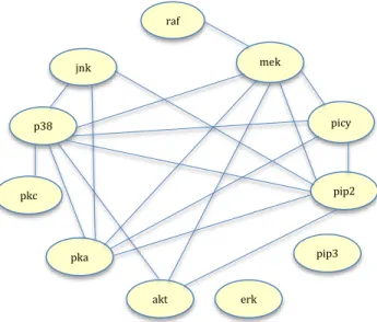
random fields. In these graphs, the absence of an edge between two vertices has a special meaning: the corresponding random variables are conditionally independent, given the other variables [18]. Figure A.5 shows an example of a graphical model for a flow-cytometry dataset with p = 11 proteins, measured on N = 7466 cells, from [23]. Each vertex of the graph corresponds to the real-valued expression level of a protein. The network structure was estimated assuming a multivariate Gaussian distribution, using the Graphical Lasso procedure discussed in the subsequent sections.
Sparse graphs have a relatively small number of edges, and are convenient for interpretation. They are useful in a variety of domains, including genomics and proteomics, where they provide rough models of cell pathways. The edges in a graph are parametrized by values or potentials that encode the strength of the conditional independence between the random variables at the corresponding vertices.
11
Figure 2.1 Example of a sparse undirected graph, estimated from a flow cytometry dataset, with p = 11 proteins measured on N = 7466 cells. The network structure was
estimated using the Graphical Lasso.
The main challenges in working with graphical models are model selection (choosing the structure of the graph), estimation of the edge parameters from data, and computation of marginal vertex probabilities and expectations, from their joint distribution. The other major class of graphical models, the directed graphical models, known as Bayesian networks, in which the links have a particular directionality (indicated by arrows), will not be studied in this thesis. A brief overview of both directed and undirected graphs can be found in [24].
Figure 2.2 Example of an undirected graphical model. Each node represents a random variable, and the lack of an edge between nodes indicates conditional independence.
For example, in the graph, c and d are conditionally independent, given b.
raf jnk p38 picy mek 1 pkc pip2 pka akt erk pip3
12
2.2.1 Graphical Gaussian Model
Here we consider Markov random fields where all the variables are continuous. The Gaussian distribution is almost always used for such graphical models, because of its convenient analytical properties. We assume that the observations have a multivariate Gaussian distribution with mean 𝝁 and covariance matrix 𝜮. The Gaussian distribution has the property that all conditional distributions are also Gaussian. The inverse covariance matrix 𝜮−1 contains information about the partial covariances between the variables; that is, the covariances between pairs i and j, conditioned on all other variables. In particular the ijth component of 𝚯 = 𝜮−1 is
zero, then variables i and j are conditionally independent, given the other variables. We now examine the conditional distribution of one variable versus the rest, where the role of 𝚯 is explicit. Suppose we partition 𝑋 = (𝑍, 𝑌) where 𝑍 = (𝑋1, . . . , 𝑋𝑝)
consists of the first 𝑝 − 1 variables and 𝑌 = 𝑋𝑝 is the last. Then we have the conditional distribution of 𝑌 given 𝑍 [25]
𝑌|𝑍 = 𝑧~𝑁(𝜇𝑌+ (𝑧 − 𝜇𝑍)𝑇𝚺
𝑍𝑍−1𝜎𝑍𝑌, 𝜎𝑌𝑌− 𝜎𝑍𝑌𝑇 𝚺𝑍𝑍−1𝜎𝑍𝑌), (2.1)
where we have partitioned 𝜮 as
𝜮 = (𝚺𝑍𝑍 𝜎𝑍𝑌
𝜎𝑍𝑌𝑇 𝜎𝑌𝑌) (2.2)
The conditional mean in (2.1) has exactly same form as the population multiple linear regression of Y on Z, with regression coefficient β = 𝚺𝑍𝑍−1𝜎𝑍𝑌. If we partition 𝚯in the same way,since 𝚺𝚯 = 𝐈standard formulas for partitioned inverses give
13 𝜃𝑍𝑌 = −𝜃𝑍𝑌∙ 𝚺𝑍𝑍−1𝜎 𝑍𝑌, (2.3) where 1/𝜃𝑌𝑌 = 𝜎𝑌𝑌−𝜎𝑍𝑌𝑇 𝚺𝑍𝑍−1𝜎𝑍𝑌 > 0. Hence β = 𝚺𝑍𝑍−1𝜎𝑍𝑌 = −𝜃𝑍𝑌/𝜃𝑌𝑌
Thus 𝚯captures all the second-order information (both structural and quantitative) needed to describe the conditional distribution of each node given the rest, and is the so-called “natural” parameter for the graphical Gaussian model 1[18].
Another (different) kind of graphical model is the covariance graph or relevant
network, in which vertices are connected by bidirectional edges if the covariance (rather than the partial covariance) between the corresponding variables is nonzero. The covariance graph however will not be studied in this thesis.
2.2.2 The Benefits of Sparsity
As pointed out in Appendix A section A.5.2.2, Lasso regularization is beneficial in that it provides an increase in prediction accuracy and allows for better interpretation. The Graphical Lasso is a method of sparse inverse covariance estimation, which offers the same benefits that lasso does for linear regression. This variable reduction capability is particularly important in portfolio optimization, where investors prefer
1 The distribution arising from a Gaussian graphical model is a Wishwart distribution. This is a
14
to invest in a smaller basket of stocks, and also in bioinformatics, when visualizing gene microarray data.
2.2.3 Inexact Methods for the Inverse Covariance Estimation 2.2.3.1 Covariance Selection Discrete Optimization
Covariance selection was first introduced by [20] as a technique for reducing the number of parameters in the estimation of the covariance matrix of a multivariate Gaussian population [20]. The belief was that the covariance structure of a multivariate Gaussian population could be simplified by setting elements of the inverse covariance matrix to be zero. Covariance selection aims at discovering the conditional independence restrictions (the graph) from a set of independent and identically distributed observations [20]. One main current of thought that underlies Covariance selection is the ‘principle of parsimony’ in parametric model fitting. This principle suggests that parameters should only be introduced sparingly and only when the data indicate they are required [18]. Parameter reduction involves a tradeoff between benefits and costs. If a substantial number of parameters can be set to null values, the amount of noise in a fitted model due to errors of estimation is substantially reduced. On the other hand, errors of misspecification are introduced if the null values are incorrect. Every decision to fit a model involves an implicit balance between these two kinds of errors [18, 20].
Covariance selection relies on the discrete optimization of an objective function. Usually, greedy forward or backward search is used. In forward search, the initial estimate of the edge set is empty, and edges are added to the set until a time where
15
an edge addition does not appear to improve fit significantly. In backward search, the edge set consists of all off-diagonal elements, and then edge pairs and dropped from the set one at a time, as long as the decrease in fit is not significantly large. The selection (deletion) of a single edge in this search strategy requires an MLE fit for
O(p2) different models [20].
The forward/backward search in covariance selection is not suitable for high-dimensional graphs in the multivariate Gaussian setting because if the number of variables p becomes moderate, the number of parameters p(p+1)/2 in the covariance structure becomes large. For a fixed sample size N, the number of parameters per data point increases (p+1)/2 as p increases. Using the technique proposed by [20], model selection and parameter estimation are done separately. The parameters in the precision matrix are typically estimated based on the model selected. Thus, parameter estimation and model selection in the Gaussian graphical model are equivalent to estimating parameters and identifying zeros in the precision matrix [26]. Applications of this sort of problem ranges from inferring gene networks, analyzing social interactions and portfolio optimization.
This sort of exhaustive search is computationally infeasible for all but very low-dimensional models and the existence of the MLE is not guaranteed in general if the number of observations is smaller than the number of nodes (variables).
2.2.3.2 Neighborhood Selection with the Lasso
To remedy the problems that arise from high dimensional graphs and computational complexity, [27] proposed a more computationally attractive method for covariance
16
selection for very large Gaussian graphs. They take the approach of estimating the conditional independence restrictions separately for each node in the graph. They show that the neighborhood selection can be cast into a standard regression problem and can be solved efficiently with the Lasso [16]. They fit a Lasso model to each variable, using the others as predictors.
The component (𝜮−1)𝑖,𝑗 is then estimated to be non-zero if either the estimated coefficient of variable i on j, or the estimated coefficient of variable j on i, is non-zero (alternatively, they use an AND rule). They show that this approach consistently estimates the set of non-zero elements of the precision matrix. Neighborhood selection with the Lasso relies on optimization of a convex function, applied consecutively to each node in the graph. This method is more computationally efficient than the exhaustive search technique proposed by [20]. They show that the accuracy of the technique presented by [20] in covariance selection is comparable to the Lasso neighborhood selection if the number of nodes is much smaller than the number of observations. The accuracy of the covariance selection technique breaks down, however, if the number of nodes is approximately equal to the number of observations, in which case this method is only marginally better than random guessing. Neighborhood selection with the Lasso does model selection and parameter estimation separately. The parameters in the precision matrix are typically estimated based on the model selected.
The discrete nature of such procedures often leads to instability of the estimator because small changes in the data may result in very different estimates [28]. The
17
neighborhood selection with the lasso focuses on model selection and does not consider the problem of estimating the covariance or precision matrix.
2.2.4 Exact Methods for the Inverse Covariance Estimation 2.2.4.1 L1- penalised methods
A penalized likelihood method that does model selection and parameter estimation simultaneously in the Gaussian graphical model was proposed by [22]. The authors employ an L1penalty on the off-diagonal elements of the precision matrix. The L1
penalty, which is very similar to the Lasso in regression [29], encourages sparsity and at the same time gives shrinkage estimates. In addition, it is ensures that the estimate of the precision matrix is always positive definite. The method presented by [22] is said to be more efficient due to the incorporation of the positive definite constraint and the use of likelihood, though a little slower computationally than the neighborhood selection method proposed by [21] due to this same constraint. They show that because the approach of [27] does not incorporate the symmetry and positive-definiteness constraint in the estimation of the precision matrix, therefore an additional step is needed to estimate either the covariance or precision matrix. [22] show that their objective function is non-trivial but similar to the determinant-maximization problem [17, 22], and can be solved very efficiently with interior-point algorithms. One problem with their approach was the memory requirements and complexity of existing interior point methods at the time, which were prohibitive for problems with more than tens of nodes.
18
A new approach of discovering the pattern of zeros in the inverse covariance matrix by formulating a convex relaxation to the problem was proposed by [30]. The authors derive two first-order algorithms for solving the problem in large-scale and dense settings. They don’t make any assumptions of known sparsity a priori, but instead try to discover structure (zero pattern) as they search for a regularized estimate. They present provably convergent algorithms that are efficient for large-scale instances, yielding a sparse, invertible estimate of the precision matrix even for N < p [30]. These algorithms are the smooth optimization method and block coordinate descent method for solving the Lasso penalized Gaussian MLE problem. The smooth optimization method is based on Nesterov’s first order algorithm [31] and yields a complexity estimate with a much better dependence on problem size than interior-point methods. The second method recursively solves and updates the Lasso problem. They show that these algorithms solve problems with greater than a thousand nodes efficiently but in experimental work, they choose to only use the smooth optimization method which is based on Nesterov’s first-order algorithm and call their algorithm COVSEL. This method has an improved computational complexity of O(p4.5 ) than previous methods.
A new method of estimating the inverse covariance was proposed by [16] using the block coordinate descent approach proposed by [30]. The authors go on to implement the block coordinate method pointed out by [30], and solve the Lasso-penalized Gaussian MLE problem using an algorithm called Graphical Lasso. Very fast existing coordinate descent algorithms enable them to solve the problem faster than previous methods, O(p3 ) [16]. Graphical Lasso maximizes the Gaussian log-likelihood
19
of the empirical covariance matrix S, through L1 (Lasso) regularization [16]. Through
regularization, the method encourages sparsity in the inverse covariance matrix, and as a consequence, demonstrates a robustness to noise, a weakness that plagues the maximum likelihood approach [16]. In the context of portfolio selection, assuming a
priori sparse dependence model may be interpreted as for example, assets belonging to a given class being related together while assets belonging to different classes are more likely to be independent. In other words, a sparse precision corresponds to covariates that are conditionally independent, so given the knowledge of a given subset, the remainder are uncorrelated.
2.3 Introduction to the Graphical Lasso
Suppose we have N multivariate Gaussian observations of dimension p, with mean μ and covariance ∑. Following [67], Let X = ∑-1 be the estimated precision matrix and
letS be the empirical covariance matrix, the problem is to maximize the log-likelihood by using a coordinate descent procedure to maximize the log-likelihood of the data [21]
𝑿̂ = arg max
𝑿 𝑙𝑜𝑔(|𝑿|) − 𝑇𝑟𝑎𝑐𝑒(𝑿𝑺) − 𝜌‖𝑿‖1 (2.4)
where S is a 𝑝 × 𝑝 empirical (sample) covariance matrix computed from observed data and X is a 𝑝 × 𝑝 symmetric and positive semi-definite matrix, which is the estimated precision matrix. ‖𝑿‖1 is the sum of the absolute values of the elements in
20
𝑿. The term 𝜌‖𝑿‖1 is known as a regularization term and 𝜌 is known as the penalty parameter. |𝑿| is the determinant of 𝑿 and 𝑇𝑟𝑎𝑐𝑒(𝑿𝑺) is the sum of the diagonal elements of the matrix product of 𝑿𝑺. Appendix B presents a detailed description of the Graphical Lasso algorithm.
The existence of the penalty term 𝜌 is what encourages sparsity in the estimated precision matrix. The practical challenge is to decide how many and which non diagonal entries in the precision should be set to zero. The Graphical Lasso presents questions such as how to select the penalty term 𝜌? When does Graphical Lasso perform well? These questions will be addressed in this thesis as they relate to the Markowitz global minimum variance portfolio optimization problem.
2.3.1 A Synthetic Data Experiment
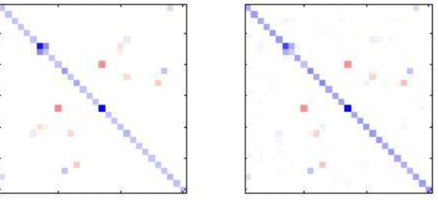
We begin with a small synthetic example showing the ability of Graphical Lasso to recover the sparse structure from a noisy matrix. Using the same data generation example for generating synthetic data as [30], the sparse structure is recovered at different regularizations ρ = (0.1, 0.4, 1, 2). The purpose of this is to see how the optimization solution changes as the regularization parameter, ρ, is increased. Starting with a sparse matrix A, we obtain S by adding a uniform noise of magnitude
σ = 0.1 to A-1. In Figure 2.3, Figure 2.4, Figure 2.5 and Figure 2.6, the sparsity pattern
of A and the optimization solution are shown. The blue colour represents positive numbers while the red represents negative numbers. The magnitude of the number is also illustrated by the intensity of the colour, with darker colours representing higher magnitudes and vice versa.
21
The purpose of this experiment is to illustrate the very important problem the Graphical Lasso method presents, which is how to effectively select the correct regularization. From Figure 2.3, Figure 2.4, Figure 2.5 and Figure 2.6, it is evident that the selection of the right amount of regularization is crucial to getting the right solution. This issue of how to select the right penalty will be addressed in this thesis as it relates to the Markowitz portfolio optimization problem in chapters 4 and 5.
Figure 2.3 Original sparse precision versus Graphical Lasso optimization solution at regularization (ρ = 0.1).
Figure 2.3 shows the Graphical Lasso solution at a regularization of 0.1. This solution appears to be very close to the original sparse precision. The diagonal elements are estimated correctly and majority of the off-diagonal elements are also estimated correctly in the solution. In Figures 2.4, Figure 2.5 and Figure 2.6, we illustrate what happens as we increase the regularization amount.
22
Figure 2.4 Original sparse precision versus Graphical Lasso optimization solution at regularization (ρ = 0.4).
Figure 2.4 shows the Graphical Lasso solution at a regularization of 0.4. We can see that the solution is worse. The diagonal elements are estimated larger, indicated by a darker diagonal, while a lot of off-diagonal elements disappear. By nature of the Graphical Lasso, as the regularization amount increases, the off-diagonals are shrunk closer to zero and this is evident in Figure 2.4. We now look at solutions for even higher regularization amounts in Figure 2.5 and Figure 2.6.
23
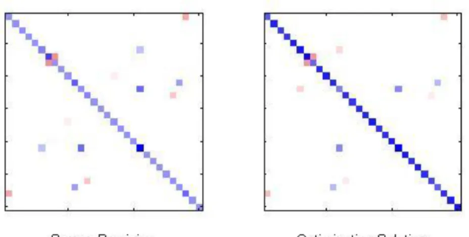
Figure 2.5 Original sparse precision versus Graphical Lasso optimization solution at regularization (ρ = 1).
Figure 2.6 Original sparse precision versus Graphical Lasso optimization solution at regularization (ρ = 2).
24
Figure 2.5 shows the Graphical Lasso solution at a regularization of 1 while Figure 2.6 shows the solution at a regularization of 2. We can see the solution gets worse as the regularization amount increases. In Figure 2.6, the off diagonal elements completely disappear, leaving very strong diagonal elements.
This experiment shows the importance of selecting the correct regularization amount, while also illustrating the issue of over-regularization, where the off-diagonal elements are shrunk too much while the off-diagonal elements are estimated too largely as the regularization amount is increased. This issue of over-regularization is addressed in section 2.4, where we introduce a new method of selecting the regularization by separately choosing regularization amounts for diagonal and off-diagonal elements.
2.3.2 A Method for Penalty Selection
Recall that Graphical Lasso solves the optimization problem given by
max
𝑿 𝑙𝑜𝑔(|𝑿|) − 𝑇𝑟𝑎𝑐𝑒(𝑿𝑺) − 𝜌‖𝑿‖1 (2.5)
where the optimal value of the penalty term 𝜌 must somehow be approximated. There are several ways that have been presented in literature on how to set the penalty 𝜌. One method called the “regression” approach fits Graphical Lasso to a portion of the data, and uses the penalized regression model for testing in the validation set [16]. Another method called the “likelihood” approach involves training the data with Graphical Lasso and evaluating the log-likelihood over the
25
validation set [16]. In chapter 4, we present new validation methods for selecting the penalty 𝜌 to obtain estimates of the inverse covariance matrix for mean-variance portfolio optimization.
This section demonstrates a method for approximating the optimal value of the penalty 𝜌. The method involves drawing a portion of data points from the training set to form a validation set and assessing the solution produced by Graphical Lasso for a number of different values of 𝜌 on this validation set. We let T denote the training set and V denote the validation set.
Algorithm 2.1 Penalty Selection 1: Select V ⊂ T 2: T’ ≔ T \ V 3:Ф ≔ { 𝜌1, 𝜌2, … , 𝜌𝑛} 4: for all𝜌𝑖 ϵ Ф do 5: 𝑿̂𝑖 = Graphical Lasso (T’, 𝜌𝑖 ) 6: 𝛶𝑖 = Fitness of Solution (V, 𝑿̂𝑖) 7: end for
8: Select 𝜌∗ = 𝜌𝑖 corresponding to maximal 𝛶𝑖
9: 𝑿̂* = Graphical Lasso ( T, 𝜌∗ )
In this thesis, the calculation of the fitness of each 𝑿̂𝑖 is achieved through the “Likelihood” approach that is offered by [16]. In this approach, the fitness of the solution of 𝑿̂𝑖 is equal to the log-likelihood given in (2.5) in which the empirical
covariance matrix 𝐒𝑉is calculated from the validation set V, providing unseen (to Graphical Lasso) information.
Fitness of Solution (V, 𝑿̂𝑖 ) = 𝑙𝑜𝑔(|𝑿̂|) − 𝑇𝑟𝑎𝑐𝑒(𝑿̂𝑖 𝐒𝑉 ) − 𝜌‖𝑿̂𝑖‖
26
This thesis and the original Graphical Lasso paper [16] use a type of validation called
k-fold cross-validation in which the training set T is randomly partitioned into k validation subsets V1,….,k each of size |𝑇|
𝑘 leaving k corresponding training sets T’1,….,k
each of size (𝑘−1)|𝑇|
𝑘 . Algorithm 3.1 is then applied k times to each Vi and T’i, and the
final selected 𝜌∗ is the average over the results of the k runs. Through k-fold
cross-validation it is hoped to minimize overfitting of the training set T. In this thesis, we use k = 5 folds (while the original paper [16] uses k = 10 folds) as a compromise between running time and overfitting.
2.4 A New Method for Penalty Selection
From the experiment in section 2.3.1, it is evident that as the regularization amount
ρ increases, the off-diagonal element values decrease, while the diagonal elements increase. There is evidence of overestimation of the diagonal elements as the solution becomes more sparse. To remedy this problem, the idea of using two different penalties is considered; one penalty for the diagonal elements, and the other for the off-diagonal elements.
2.4.1 The Model
Graphical Lasso maximizes the L1- log likelihood equation,
27
To correct the problem of overestimation of the diagonal, expression (2.7) is modified to the following
𝑙𝑜𝑔(|𝑿|) − 𝑇𝑟𝑎𝑐𝑒(𝑿𝑺) − 𝜌1‖𝑿‖1{𝑖≠𝑗}− 𝜌2‖𝑿‖1{𝑖=𝑗} (2.8)
From (2.8) we can see that two different penalties will be chosen; one for the off-diagonal elements (𝜌1), and the other for the diagonal elements (𝜌2). This new algorithm will be referred to as the Modified Graphical Lasso.
To approximate the penalties 𝜌, 𝜌1and𝜌2, a method involving cross validation is used. This method, described in section 2.3.2, Algorithm 2.1 involves drawing a portion of data points from the training set to form a validation set and assessing the solution produced by both Graphical Lasso and the Modified Graphical Lasso for a number of different values of 𝜌, 𝜌1and𝜌2 on the validation set.
The possible regularizations amounts chosen for 𝜌, 𝜌1and𝜌2 are the same range of 20 different values from 0 to 1000. For the Modified Graphical Lasso, all possible combinations of 𝜌1and𝜌2 are considered. The optimal choice of 𝜌, 𝜌1and𝜌2 are picked based on maximum likelihood/largest fitness. The fitness of the solution 𝑿̂ is equal to the log-likelihood given in (2.7) and (2.8), in which the empirical covariance matrix is calculated using the validation set.
Fitness of the Graphical Lasso solution is given by
𝑙𝑜𝑔(|𝑿̂|) − 𝑇𝑟𝑎𝑐𝑒(𝑿̂𝐒𝑉) − 𝜌‖𝑿̂‖
28
Fitness of the Modified Graphical Lasso solution is given by
𝑙𝑜𝑔(|𝑿̂|) − 𝑇𝑟𝑎𝑐𝑒(𝑿̂𝐒𝑉) − 𝜌1‖𝑿̂‖
1{𝑖≠𝑗}− 𝜌2‖𝑿̂‖1{𝑖=𝑗} (2.10)
Synthetic data experiments are performed to show how the Modified Graphical Lasso performs compared to the Graphical Lasso, and the results are shown in the subsequent sections. 5-fold cross validation is used to train and test the data and calculate the likelihood and the optimal regularizations. We use the Moore-Penrose pseudoinverse (introduced in Appendix A) as a baseline method for comparison.
2.4.2 Generating Synthetic Data
To implement the new penalty selection method, synthetic data is generated according to the following models:
Model 1: A sparse model taken from [22] (X)i,i= 1, (X)i,i-1= (X)i-1,i=0.5, and 0 otherwise.
The diagonal elements of X are equal to 1 and the elements next to each diagonal entry equal to 0.5. All other elements are equal to 0.
Model 2: A dense model taken from [22] (X)i,i = 2, (X)i,i’= 1 otherwise.
29
For each model, we simulated i.i.d Gaussian samples of sizes (𝑁 = 5, 10, 20, . . . , 100)
and for different variables sizes (p =10, 30, 50, 70) according to Algorithm 4.1.
2.4.3 Performance Measure
The performance of the original Graphical Lasso is compared to the Modified Graphical Lasso across different variable (p =10, 50, 70) and sample sizes (N = 5 to 100). For both the sparse and dense models, we know the true precision, 𝑿. Algorithm 2.1 is used to approximate the optimal 𝜌∗, 𝜌1∗ and 𝜌2∗, and the corresponding optimal estimated precision, 𝑿̂. The difference between 𝑿̂ and𝑿 is then quantified using the Frobenius norm ‖𝑿̂ − 𝑿‖
𝐹, defined for an M x N matrix Aas
||𝑨||𝐹 = √ ∑ ∑ 𝑨𝑚𝑛2 𝑁 𝑛=1 𝑀 𝑚=1
Using the pseudoinverse as a baseline method for comparison, we expect that the Graphical Lasso and Modified Graphical Lasso will both perform better than the baseline pseudoinverse method for the sparse model. This is due to the fact that by nature, Graphical Lasso assumes a sparse model, and in such situations is expected to be a better approximation of the actual inverse covariance matrix than ordinarily inverting the covariance matrix or using its pseudoinverse. For the dense model, we expect the pseudoinverse to perform well especially at very high sample sizes relative to the number of variables.
30
2.5 Experiment Results
2.5.1 Model 1 Results
A sparse model: (X)i,i= 1, (X)i,i-1= (X)i-1,i=0.5, and 0 otherwise.
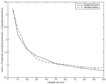
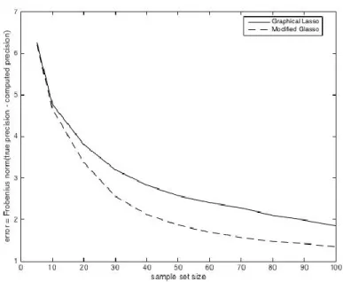
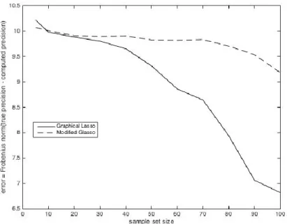
Figure 2.7 Model 1 error between Graphical Lasso and Modified Graphical Lasso (p =10).
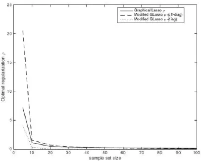
Figure 2.8 Model 1 optimal penalty for Graphical Lasso and Modified Graphical Lasso (p =10).
31
From Figure 2.7, it appears that at certain sample sizes, the Modified Graphical Lasso performs better than the original Graphical Lasso, having lower error. Statistical hypothesis tests (t-tests) are performed to verify these results and are presented in Appendix E. For better viewing, we present the actual values of the error and optimal regularizations for the Modified Graphical Lasso, the Graphical Lasso and the pseudoinverse in Appendix E also. Based on the results of the hypothesis tests in Appendix E Table E.1, for the sparse model at 𝑝 = 10, the two methods perform essentially the same, except when 𝑁 > 70 where the original Graphical Lasso performs statistically significantly better than the modified Graphical Lasso. The pseudoinverse performs worse than the Graphical Lasso and Modified Graphical Lasso as expected in this sparse scenario, although its performance gets better as the number of samples increase.
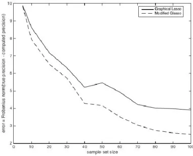
Figure 2.9 Model 1 error between Graphical Lasso and Modified Graphical Lasso (p =30).
32
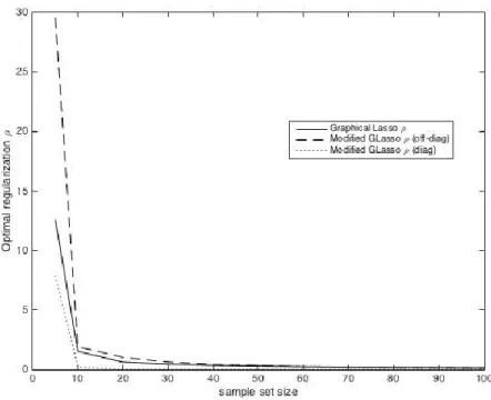
Figure 2.10 Model 1 optimal penalty for Graphical Lasso and Modified Graphical Lasso (p=30).
Figure 2.11 Model 1 error between Graphical Lasso and Modified Graphical Lasso (p =50).
33
Figure 2.12 Model 1 optimal penalty for Graphical Lasso and Modified Graphical Lasso (p=50).
Figure 2.9 shows the error across different samples for the sparse model when p=30, while Figure 2.11 shows the error across different samples for the sparse model when
p=50. In these two figures, the Modified Graphical Lasso method appears to perform better than the Graphical Lasso method. Statistical hypothesis tests in Appendix E Table E.3 and Table E.5 however show that the two methods perform essentially the same across all samples, and both methods perform better than the pseudoinverse across all sample sizes. We now examine a larger variable size (p=70).
34
Figure 2.13 Model 1 error between Graphical Lasso and Modified Graphical Lasso (p =70).
Figure 2.14 Model 1 optimal penalty for Graphical Lasso and Modified Graphical Lasso (p =70).