Methodology for Timing and Impact Analysis of
Signalized Intersections
Karl Bang
1, Johan Wahlstedt
2and Leif Linse
3 1The Royal Institute of Technology (KTH), Stockholm, Sweden.2Ramboll Sverige AB, Stockholm, Sweden. 3
Trivector Traffic AB, Malmo, Sweden
klbang@abe.kth.se, johan.wahlstedt@ramboll.se, leif.linse@trivector.se,
Abstract
A new Swedish capacity manual has been developed based on a major research project called METKAP. This paper is focused on the deterministic methods for calculation of signal timing and traffic performance measures for isolated, fixed time signalized intersections documented in the new manual (STA 2013a) and applied in the CAPCAL 4 software (Linse 2013). The use of the methods is mandatory in projects for the Swedish Transport Administration (STA). Special focus has been devoted to the following issues: 1) Modelling of saturation flow for opposed lanes. 2) Impact of short approach and exit lanes. 3) Iterative signal timing process based on critical conflict identification, intergreen and minimum green times.
The deterministic methods can also be applied for selection of maximum green time for VA-controlled intersections, and as planning tool for analysis of the traffic performance alternative intersection types, designs. They can also be used to identify “bottleneck intersections” and for determination of minimum cycle time and required green time ratios for coordinated traffic signal systems.
Micro simulation can be used as an alternative method, e.g. to model complex, signal control strategies and active priority of public transport vehicles. Need for simulation also arises if adjacent traffic facilities influence the studied system, and for animation purposes. However, micro simulation has important short-comings compared to deterministic methods. Simulation models require validated and detailed input data, e.g. regarding vehicle characteristics, arrival distribution, route choice and driver behavior. It is also difficult to estimate saturation flow, capacity and volume-to-capacity ratio since the simulated queue discharge is normally based on car-following models. Determination of optimal intersection design and signal timing requires a very large number of simulation runs and is therefore very time consuming and costly.
Keywords:Methodology, Signal timing, Capacity, Traffic performance, Software
Volume 15, 2016, Pages 75–86
ISEHP 2016. International Symposium on Enhancing Highway Performance
1 Introduction
A detailed methodology for signal timing and capacity analysis of signalized intersections was developed in the seventies as a part of a new Swedish Capacity Manual (SRA 1977) by Bang (1978). Computational aids for this method were also developed in the form of the CAPCAL software, which has later been subject to a number of updates including traffic safety, emission and other performance measures for all major types of at-grade intersections (Hagring et al 2010). A new Swedish capacity manual has since been published (STA 2013a) based on major research and development projects (Hagring 2000; Al-Mudhaffar 2006, Wahlstedt 2011, Bang 2014). This paper is focused on revised deterministic methods for calculation of signal timing and traffic performance measures for isolated, fixed time signalized intersections documented in the new manual (METKAP) and applied in CAPCAL 4 software (Linse 2013). Special focus has been devoted to the following issues:
x Detailed modelling of saturation flow for opposed lanes.
x Short lane utilization and contribution to approach bottleneck capacity
x Inter-green times and minimum green periods and their application in the signal timing process.
x Procedures for finding the critical conflict point between conflicting traffic movements as a basis for determination of optimal signal timing.
The paper is concluded with a discussion regarding the use of simulation as an alternative method.
2 Overview of the Methodology
The capacity of a signalized intersection approach is primarily a function of number of lanes and their traffic flow, directional distribution, saturation flow and green time ratio. Saturation flow for a lane depends on its geometry and degree of conflict with opposing vehicle and pedestrian movements that are discharged in the same signal phase. Since the signal timing is not known from the start, iterative calculations must be performed starting from base assumptions regarding cycle time, lost time and green time distribution as a function of intersection type. The obtained signal timing is then applied for new calculations of traffic lane distribution, ratio of turning traffic, saturation flow, critical conflict point, signal timing and resulting flow discharge and capacity in the next iteration.
Figure 1: Overview of the calculation process for signalized intersections Initial calculation (Approximate results)
Determine lane type and flow for each lane (q)
Determine intergreen and select initial values for signal timing
Determine saturation flow (s) and load factor (q/s) for all bottleneck lanes Identify the critical conflict point for main phase flows
Determine total lost time (F), cycle time (c)and green times (g)
Revise signal timing if calculated g < gmin
Determine capacity (C)and degree of saturation (DS)for all lanes Iteration 2 … n
Check phase scheme, lane types, minimum green, inter-green, lost time Repeat all calculations using the resulting values for signal timing, traffic flow and saturation flow for each lane from the previous iteration. Impact analysis
Traffic performance impacts (delay, queue length, ratio of stopped veh.) Environment, safety and cost impacts. Analysis for oversaturated conditions
The METKAP development has been supported and tested by programming the algorithms in MsExcel (STA 2013b). The principal signal timing method for fixed time control was first proposed by Webster (1958) and Webster and Cobbe (1966) and further developed by Bang (1978 and 2014). The resulting signal settings are used in METKAP as a basis for determination of maximum green times (gmax)and extension intervals for traffic actuated control. However, care must be taken to avoid
too high cycle times at high degrees of saturation causing increased vehicle and pedestrian delay.
3 Determination of Saturation Flow
3.1 General Methodology
Saturation flow (s) for a signalized lane is defined as stationary traffic flow at queue discharge (vehicles per hour of green: vphg). Many factors influence s: 1) Geometric design (lane width and length, rise/fall, curve radius); 2) Ratio of left and right turning traffic; 3) Degree of conflict with opposing vehicle movements and/or pedestrian flows at crosswalks that have green in the same phase. The models and calculation processes for determination of s for all these cases are handled by development of models for different lane types A – D (STA 2013):
Type A: Unopposed straight through traffic movement
Type B: Unopposed mixed straight and turning traffic movement
Type C: Opposed left- or right-turning traffic movement (vehicle-pedestrian conflicts) Type D: Opposed left-turning traffic movement (vehicle – vehicle conflicts)
Saturation flow for a lane may have to be tested for both lane type C and D if the left-turning movement first faces a conflict with opposing vehicles, and then crosses a crosswalk with green in the same phase. The resulting
s
for such a lane will be equal to MIN(sC; sD).Depending on the design andsequence of signal phases the same lane may operate both as lane type B in a phase when both the opposing vehicle and pedestrian movements have red, and as lane type C and D.
Saturation flow modelling for lane type C (pedestrian conflict)
Figure 2 Analysis of saturation flow for lane type C (opposed pedestrian conflict)
During period A and B no turning vehicle can pass the crosswalk due to pedestrian platoons, during B and D passage can occur in gaps between randomly arriving pedestrians. The number of turning vehicles (Ng)can pass per green phase can be estimated as
Time Space
Pedestrian trajectories
Green time
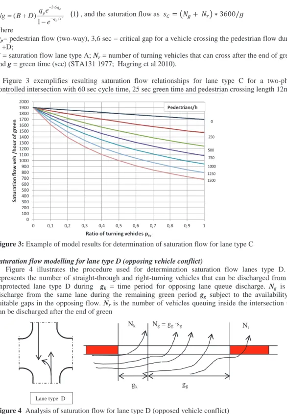
3.6 / ' ( ) 1 p p q p q s q e Ng B D e
ͼ1ͽ, and the saturation flow as ݏ =൫ܰ+ ܰ൯ כ3600/݃ ͼ1ͽ
where
qp= pedestrian flow (two-way), 3,6 sec = critical gap for a vehicle crossing the pedestrian flow during
B +D;
s’= saturation flow lane type A; Nr= number of turning vehicles that can cross after the end of green,
and g= green time (sec) (STA131 1977; Hagring et al 2010).
Figure 3 exemplifies resulting saturation flow relationships for lane type C for a two-phase controlled intersection with 60 sec cycle time, 25 sec green time and pedestrian crossing length 12m.
Figure 3:Example of model results for determination of saturation flow for lane type C
Saturation flow modelling for lane type D (opposing vehicle conflict)
Figure 4 illustrates the procedure used for determination saturation flow lanes type D. Nk
represents the number of straight-through and right-turning vehicles that can be discharged from the unprotected lane type D during gk = time period for opposing lane queue discharge. Ng is the
discharge from the same lane during the remaining green period gg subject to the availability of
suitable gaps in the opposing flow. Nris the number of vehicles queuing inside the intersection that
can be discharged after the end of green
Figure 4 Analysis of saturation flow for lane type D (opposed vehicle conflict)
0 100 200 300 400 500 600 700 800 900 1000 1100 1200 1300 1400 1500 1600 1700 1800 1900 2000 0 0,1 0,2 0,3 0,4 0,5 0,6 0,7 0,8 0,9 1 Sa tu ra ti on f low v eh /h our of g re en
Ratio of turning vehicles psv
0 250 500 750 1000 1250 1500 Pedestrians/h Lane type D gg gk Nk Ng= ggÂsg Nr
The dischargeNkdepends on length of gkand number of left-turning vehicles Nlqthat can queue
inside the intersection without blocking the straight-through or right-turning vehicles from this lane. ݃=ݍή ݎ/(ݏെ ݍ)
where
qois opposing traffic flow per lane; sosaturation flow, androthe red time of the opposing flow.
IfNlq= 0, ࡺ = σୀଵୀேିଵ[(݅ ή )ή(1െ )]+ ܰ ή(1െ ே) ͼ2ͽ
where
N = NK, max= gkÂ; pl=ratio of left-turning vehicles in the opposed lane. IfNlq=1
ࡺ=σ [݅ ή(݅+ 1)ή ଶή(1െ
)] ୀேିଶ
ୀଵ + (ܰ െ1)ή ܰ ή ή(1െ )(ேିଵ)+ܰ ή(1െ )ே
ͽ
ͼ3ͽThe discharge Ngduring the remainder of the green phase with random arrivals of opposing
vehicles can be estimated as
Ng = sg· gg;
s
g,pl=1 = (,ήషೌή,) (ଵିషೌή,); s
g,pl<1= ଵ ( ೞసభା (భష) ೞಲ )
ͼ4ͽ where
qo,tot
=
Total opposing flow veh/sec ;ag = Critical gap (sec);af = time headway for a vehicle discharged in the same gap;
pl ratio of left-turning vehicles in the opposed lane type D; and sA
=
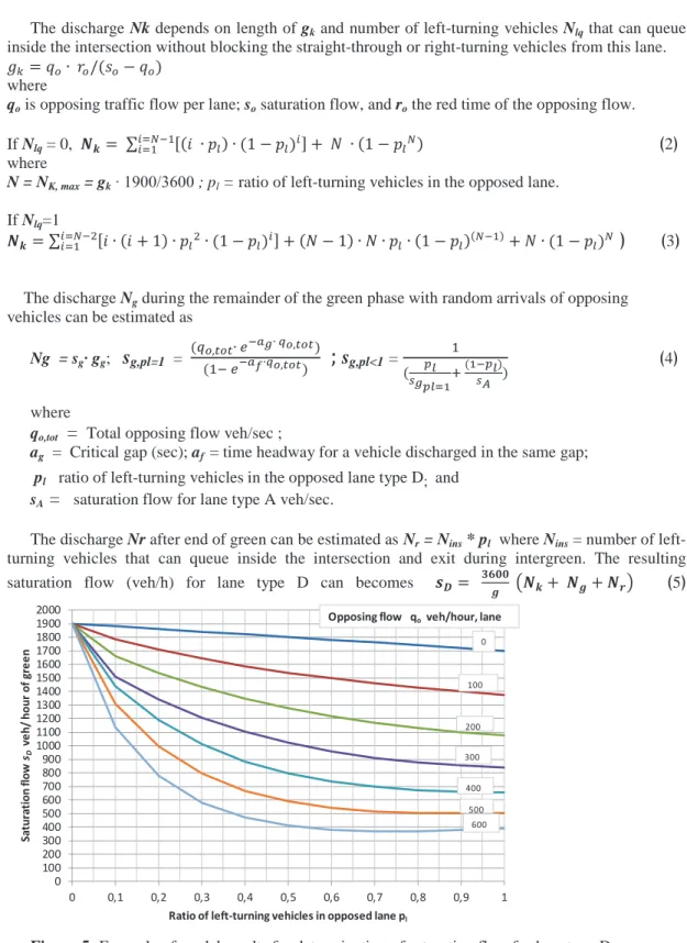
saturation flow for lane type A veh/sec.The discharge Nrafter end of green can be estimated asNr= Nins* pl where Nins= number of
left-turning vehicles that can queue inside the intersection and exit during intergreen. The resulting
saturation flow (veh/h) for lane type D can becomes ࢙ࡰ=
ࢍ ൫ࡺ+ ࡺࢍ+ࡺ࢘൯ ͼ5ͽ
Figure 5:Example of model results for determination of saturation flow for lane type D 0 100 200 300 400 500 600 700 800 900 1000 1100 1200 1300 1400 1500 1600 1700 1800 1900 2000 0 0,1 0,2 0,3 0,4 0,5 0,6 0,7 0,8 0,9 1 Sa tu ra ti on f low sD ve h/ hour of gre e n
Ratio of left-turning vehicles in opposed lane pl
100 200 300 400 500 600
Opposing flow qoveh/hour, lane 0
3.2 Impact of Short Lanes
Short lanes for right or left turning movements in approaches to signalized intersections are very common in Sweden (Case A). Short lanes are also frequent in exit arms (Case B), see Figure 7 below.
Case A: Short lane contribution to approach capacity
A short lane is defined as a lane that does not contribute fully to traffic discharge during normal traffic conditions because of its restricted length, i.e. the lane will be empty before the adjacent lane even at fully saturated conditions. The latter lane is here called the bottleneck lanesince it determines the possible total saturation flow for both lanes. The number of vehicles discharged from a short lane per signal cycle is taken into account as increased approach capacity through calculation of a
contributionto the bottleneck lane saturation flow. The signal timing (see Chapter 4) then determines the capacity of the approach. A number of different short lane cases for determination of this contribution can be identified:
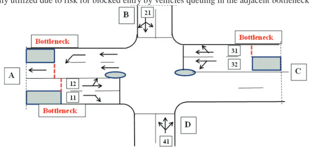
Case A-1:The short lane serves only turning traffic and is discharged in the same phase as the adjacent bottleneck lane. The short lane 11 in Figure 6 serves only right-turning traffic and may not be fully utilized due to risk for blocked entry by vehicles queuing in the adjacent bottleneck lane 12.
Figure 6: Illustration of short lanes and corresponding bottlenecks
The saturation flow contribution to lane 12 provided by the short lane 11 is based on the number of vehicles at saturated conditions that can queue in this lane during red signal before further entry is blocked by queuing vehicles in lane 12. This flow contribution depends on the following factors: x Ratio of right turning vehicles (pr) in the bottleneck lane
x Phase sequence during a signal cycle controlling entry of queuing vehicles to the short lane x Maximum number of vehicles that can queue in the short lane: Nmag=lsl,/lvehwhere lslrepresents
the length of the short lane in meters and lvehvehicle spacing during queuing (normal 8 m for pc)
x Number of vehicles (Nqueue, block) that can queue in the short lane before it is blocked by queue in
the bottleneck lane. The resulting value is obtained with equation 10 or Figure 8 below. x The number of vehicles (Nqueue,flow) that can enter the short lane depending on red time rfor the
bottleneck lane and flow (qsv) of turning vehiclesNqueue,flow= r * qsv/3600. ͼ6ͽ
x The resulting number of queuing vehicles in the short lane is determined as
Nqueue= min(Nqueue,block ; Nqueue,flow). ͼ7ͽ
x The saturation flow contribution of the short lane to the adjacent bottleneck lane is calculated as Vƍ NqueueÂ
With two-phase control in a four-arm intersections as shown in Figure 6 discharge of the approaches A and C with short lanes can take place during green time in phase 1, and queuing occurs during red time in phase 2. The number of vehicles that can enter a short lane for turning vehicles during saturated conditions and red signal in the approach can be calculated as follows:
ଵ+ଶ= 1
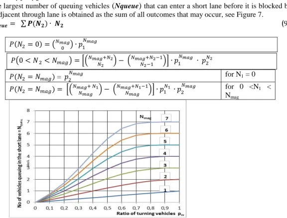
The largest number of queuing vehicles
(
Nqueue)
that can enter a short lane before it is blocked by the adjacent through lane is obtained as the sum of all outcomes that may occur, see Figure 7.ࡺ࢛ࢋ࢛ࢋ= σ ࡼ(ࡺ)ή ࡺ ͼ9ͽ ܲ(ܰଶ= 0) =൫ேೌ ൯ ή ଵ ேೌ ܲ(ܰଶ=ܰ)= ଶேೌ for N1= 0 ܲ(ܰଶ=ܰ) = ቂቀேೌାேభ ேೌ ቁ െ ቀ ேೌାேభିଵ ேೌ ቁቃ ή ଵ ேభ ή ଶ ேೌ for 0 <N1 < Nmag
Figure 7: Number of queuing vehicles Nqueue that can enter a short lane during saturated conditions Case A-2: The short lane serves both turning and through traffic (e.g. lane 32 in Figure 6).
If the short lane has green in the same phase as the adjacent bottleneck lane and also serves through traffic it will not be blocked by queuing vehicles in the adjacent lane. The saturation flow contribution from the short lane will then be restricted by the green time and the number of vehicles that can queue in the short lane:
1. Determine the saturation flow sof the short lane without consideration to its length. 2. Determine the maximum number of vehiclesNgthat can be discharged from the short lane
during the green time g: Ng = g*s/3600 (in iteration 1 use base assumption for g). 3. Determine the number of vehicles Nmagthat can queue in the short lane.
4. Determine saturation flow contribution s’ of the short lane to the bottleneck lane
Nqueue =Min(Ng; Nmag) s’ =Nqueue*3600/g ͼ10ͽ
Nmag Maximum no of vehicles that can queue in the short lane (lane 2)
N1 No of queuing vehicles in the adjacent lane (lane 1=bottleneck)
N2 No of queuing vehicles in the short lane (lane 2)
P(N2) Probability for N2queueing vehicles in lane 2
p1 Probability of vehicles in the bottleneck that cannot use the short lane
p2 Probability of turning vehicles in the bottleneck that can use the short lane
ܲ൫0 <ܰଶ<ܰ൯=ቂቀேೌାேమ ேమ ቁ െ ቀ ேೌାேమିଵ ேమିଵ ቁቃ ή ଵ ேೌ ή ଶேమ
Case A-3: The short lane serves only turning traffic in a separate phase after the phase with green for the adjacent bottleneck lane.
This case is unusual since the queue of turning vehicles trying to enter the short lane may block the through traffic in the bottleneck lane. The saturation flow contribution to the bottleneck lane in this
case is determined as s’ =Nmag*3600/g . ͼ11ͽ
Saturation flow determination for Case A approach bottleneck lanes One lane bottlenecks (Approach A in Figure 6)
1) The of ratio of left- and right turning vehicles in the bottleneck lane upstream of short lanes is calculated based on the total flow in the approach as =ݍ/ݍ௧௧;=ݍ/ݍ௧௧
2) The saturation flow of the bottleneck lane in the same section is calculated as
࢙=൫࢙࢚࢟ࢋ,,࢙࢚࢟ࢋ,࢘,࢙࢚࢟ࢋࡰ,൯+࢙Ԣ)vehicles/hour of green, ͼ12ͽ
i.e. as the lowest svalue for all involved lane types + contributions’from short lane(s). Multiple lane bottlenecksSaturation flow for each bottleneck lane is calculated based on the same principles as for the one-lane case. The distribution of the approach flow between these lanes is calculated based on obtaining the same q/s ratio for each bottleneck lane.
Case B: Impact of short lanes and bottlenecks in intersection exit arms
Short lanes are also common in intersections exits, see Figure 6 exit A. In this case the short lane does not contribute to the exit bottleneck saturation flow, but provides additional capacity since the period for fully saturated discharge through the bottleneck is prolonged. However, the risk for blockage of the intersection by queuing vehicles from the studied exit must be considered as follows:
x The length of the exit short lane should preferably be longer than the mean queue length in the approach with the highest flow and the same number of lanes leading into the studied exit.
x The capacity of the exit bottleneck must exceed the total flow from all traffic movements leading into this approach. The degree of saturation for the bottleneck should therefore not be higher than 0.8 during peak hour flow conditions.
x The merging of vehicles from the exit short lane to the exit bottleneck lane should be facilitated through signing permitting “zipping” between vehicles from both lanes.
3.3 Determination of Load Factor (q/s)
The results from sections 3.1 and 2 above are used to calculate the following results: Saturation flow (s) smin for the lane in each approach and phase with the lowest value
Traffic flow (q) For approaches with multiple lanes serving traffic in the same direction of travel the traffic flow per laneqi is determined assuming that the drivers select the lane
which results in minimum delay, i.e. the load factor for these lanes will be equal Load factor (qi/smin) The lanes with the highest load factor in each phase are selected for
determination of the critical conflict point, see Section 4.2 below.
4 Signal Timing Analysis
The signal timing process includes the following steps:
x Determination of inter-green time periods needed to separate primary conflicts between conflicting traffic movements (in two-phase control only primary conflicts).
x Determination of total lost time per cycle
x Determination of minimum green periods for vehicle and pedestrian movements
x Determination of cycle time and green times for all phases
x Calculation of degree of saturation and capacity
4.1 Intergreen, Lost Time and Minimum Green
CAPCAL includes calculation of intergreen (amber, all-red and red-amber time) and minimum green times according to Swedish rules. The intergreen times mainly depend on the geometry of the intersection. The dimensions of the intersections are entered and the distances from the stop lines to conflict points and lengths of crosswalks are automatically calculated for a normal 90 degree intersection. The sum of the intergreen times is equal to the total lost time per cycle (L), i.e. time needed for safety reasons to separate traffic movements with crossing conflict. Drivers in the “dilemma zone” who are unable to stop before the stop line may pass it during amber. This part of the amber signal can therefore be considered as an addition to effective green, and the remaining part as an addition to L.According to Swedish regulations the red timesRshall be calculated individually for each conflict point as ܴ= ࢉ࢜ା࢜
ࢉ െ
ࢋ
࢜ࢋെ ܴܣ
ͼ
13ͽ
where
ࢉ= distance from stop line to conflict point for clearing vehicle, crosswalk length for pedestrian ࢜= length of dimensioning vehicle (pedestrian = 0m, bike = 2m, car = 6m, bus = 15m)
࢜ࢉ= speed of clearing vehicle, max allowed according to table, 1,4 m/s for pedestrian ࢋ= distance from stop line to conflict point for entering vehicle, zero for pedestrian ࢜ࢋ= speed of entering vehicle, min allowed according to table
RA= red-amber time for entering (pedestrian = 0s, vehicle = 1,5s)
The required minimum green time per main phase is equal to the longest minimum green time of the lanes or crosswalks served in the phase. Thus the minimum green time for vehicle lanes is 6 seconds and minimum green time for crosswalks are calculated as:
ࢍ=࢜ࢉ࢘
ࡼࢋࢊ
ͼ
14ͽ
where
ࢉ࢘= length of the whole crosswalk curb to curb;࢜ࡼࢋࢊ= pedestrian speed, max 1,4 m/s
4.2 Identification of the Critical Conflict Point
The main purpose of traffic signals is to time-separate conflicts between through traffic movements from crossing streets (primary conflicts). Time separation can also be applied between turning and opposing straight-through movements (secondary conflicts), and between turning vehicle movements and pedestrian crossings if needed for safety or capacity reasons.
Figure 8 illustrates a conflict point for an intersection with three main phases. The arrows represent the lane in each phase with the highest load factor (q/s) as described in Section 3.3. The total of the load factors for the main phases jin the critical conflict pointis the highest sum obtained: ܯܣܺ σ(ݍ݆
ݏ݆
ൗ )
ͼ
15ͽ
If the signal control includes alternative extra phases the phase sequence that gives the highest load factor sum including one of these alternative phases is used for identifying the critical conflict point. A new search for the critical conflict point must be undertaken at every signal timing iteration because of changes of saturation flow and lane flow estimates incurred by revised signal timing.Figure 8 Critical conflict point for an intersection with three main phases.
4.3 Signal Timing
Webster (1958) has shown that the cycle time cthat results in minimum average vehicle delay can be calculated using equation (17) as whereand are constants and Ltotal lost time per cycle
c
=
భήାమήହଵିσ(
ೞ )ೌೣ
ͼ
16ͽ
If the sum of the load factors in the denominator becomes close to one, the resulting cycle time will exceed values that are too high to implement. In Sweden the limit for cycle time is normally 120 seconds. The design and/or phasing of the intersection then need to be changed.The green time gjin each phase jis computed as gj= (c–LÂįj whereįjis the green time ratio.ࢍ= [(ࢉ െ ࡸ)ή]ࢾ= [ࢉ െ ࡸ]ή
(/࢙)ࢇ࢞
σ(/࢙)ࢇ࢞
ͼ
17ͽ
Ifࢍ< ࢍ,, the minimum green time is applied and a new total lost time is calculated as
Lcorr= L + [gx,min - gx] ,i.e. the green time addition to satisfy the minimum green time criteria is added as lost time. A revised cycle time is calculated as ccorr=
,ήࡸ࢘࢘ା
ିσ(
࢙ )ࢇ࢞
ͼ
18ͽ
New green times gj,korrare then calculated as gj,corr=(ccorr –LÂįj.ͼ
19ͽ
If the adjusted green times is still too low for one or more phases the process above is repeated until all minimum green times are satisfied.
4.4 Capacity and Degree of Saturation
The capacity for lane i with green in phase j is calculated as = ࢍ
ࢉ ή ࢙, and the degree of saturation ࡰࡿ=
The signal timing described above results in the same DS for all traffic
movements passing the critical conflict point, which is a prerequisite for obtaining minimum total intersection delay at a given level of demand. However, DSfor lanes that obtain extended green times as a result of the minimum green time corrections will normally be lower than for the other lanes that are included in the critical conflict point.
5 The CAPCAL Software
CAPCAL is a software product designed for determination of capacity and measures of performance for all types of at-grade intersections (Hagring 2000 and 2010). The latest version, CAPCAL 4 (Linse 2013), is based on the METKAP models (STA 2013a). The Capcal program is has a shared ownership between Swedish Transport Administration (STA) and Trivector. CAPCAL has
users in Sweden, Finland, Norway and Iceland. It is commonly used to check performance levels required by national guidelines as well as comparing different intersection designs and signal control regarding traffic performance and annual costs for accidents, emissions and delay.
CAPCAL 4 has two main parts, the calculation engine and the user interface which allows users to define intersections, trigger calculation and read out results. The user interface also has an updated module for comparison of different scenarios including graphs and tables. The software automatically identifies main phases and extra phases defined in METKAP (STA 2013 a) using a heuristic method specially developed for the computer implementation. If multiple extra phases are assigned to the same main phase, CAPCAL 4 will consider them as alternative extra phases and activate at most one of them in the capacity calculation.
In CAPCAL 4 intergreen and minimum green times are recalculated immediately after change of any design input field. The results are based on automatically updated intergreen times as different lane configurations are tried, but the user is also free to override this, e.g. using existing documented signal timing documentation are preferred.
After capacity and DS of the intersection have been calculated, CAPCAL 4 computes queue lengths and delay, as well as socioeconomic effects such as costs due to emissions and accidents. The software also includes a module for oversaturated intersections that is used for long-term life-cycle impact evaluations and comparisons of intersections types and designs. All modules are used by all intersection types, but there are some specific formulas and methods for traffic signals, e.g. for delay and queue length. The calculation of impacts such as emissions, time cost and accidents are based on standardized Swedish parameters and models issued by the government. The final result of these calculations is a monetary cost for society which can be used to compare different intersection designs.
6 Use of Deterministic and Simulation Methods for Traffic
Signal Analysis
Deterministic methods as documented in HCM2010 (TRB 2010) and the Swedish manual (STA 2013a) use constant parameters (e.g. demand, saturation flow, critical gaps based on empirical knowledge) for analysis of isolated, fixed time controlled intersections. Mean, empirically based estimates of saturation flow for all lane types can be calculated for determination of the critical conflict point, optimal fixed signal timing, capacity and traffic performance using deterministic capacity software such as CAPCAL, HCS and SIDRA. The capacity of an isolated intersection with vehicle actuated signal control (VA) normally converges to fixed-time (FT) results at higher degree of saturation (Bang 1976, Al-Mudhaffar 2006). Delay and other impacts for VA-controlled signals can be approximated using correction factors. The deterministic methods can therefore also be applied as basis for determination of optimal timings for VA-controlled intersections. Moreover they can be used as planning tools for analysis of alternative intersection types, designs, signal phasing and estimation of traffic performance. The deterministic methods also simplify timing of coordinated signal systems since they can be used to identify the “bottleneck intersections” for determination of minimum cycle time as well as required green time ratios for all intersections in the system.
Simulation methods can be used to model the performance of complex, signal control strategies and systems that deterministic methods cannot handle, e.g. including real time self-optimization and/or active priority of public transport vehicles. Need for simulation can also arise if the studied intersection is not isolated, i.e. adjacent intersections or road links can cause blockage and influence the discharge (Wahlstedt 2013), or if the signal control includes active bus priority (Wahlstedt 2011). Micro simulation software (e.g. VISSIM, AIMSUN) uses stochastic demand and driver behavior variables for modelling the variability and uncertainty of the traffic process. The analysis can be
descriptive, e.g. how traffic will behave in a given situation, or normativee.g. if embedded logic in the simulation software emulates the studied signal control strategy explicitly (TRB 2010). Simulation can be used for study of single intersections, coordinated signal corridors or area traffic signal control including adjacent traffic facilities that could influence the studied system. Simulation also enables animation of the traffic process for demonstration of how the traffic system will function at different levels of demand.
Micro simulation has a large potential for many traffic signal analysis tasks, but also important shortcomings compared to deterministic methods. Simulation models require validated, detailed input data, e.g. regarding arrival distribution, route choice and driver behavior characteristics. It is difficult to estimate saturation flow, capacity and volume-to-capacity ratio since the simulated queue discharge is normally based on car-following models. Determination of optimal signal phasing and timing is therefore very complex, time-consuming and costly since it requires a very large number of simulation runs with different signal settings and other assumptions.
References
Al-Mudhaffar, A. (2006) Impacts of Traffic Signal Control Strategies. Part II: Impacts of Isolated Signal Control Strategies with LHOVRA Technique. Royal Institute of Technology (KTH), Report TRITA-TEC-PHD 06-005 2006.
Bang, K.L. (1976) Optimal Control of Isolated Traffic Signals. Transportation Research Record No. 597, TRB Washington D.C.
Bang, K.L. (1978) Swedish Capacity Manual Part 3: Capacity of Signalized Intersections. Transportation Research Record 667, Washington D.C.
Bang, K.L. (2014) Methods for Capacity Analysis. Part 3: Signalized Intersections (in Swedish) KTH report TRITA-TSC-RR 14-016, ISBN 978-91-87353-61-1) Stockholm 2014
Hagring, O. (2000) Accessibility in Intersections with Traffic Signals. Report 191, LTH, Lund University Sweden.
Hagring, O., Allstrom A. (2010) CAPCAL 3.3.Model Description of Intersections with Signal Control. Trivector AB Lund Sweden 2010
Linse, L. (2013) CAPCAL 4 User Manual. Trivector 2013:87, Lund, Swednn 2013 SRA (1977) Calculation of Capacity, Queue Length and Delay in Road Traffic Facilities (in Swedish), Swedish Road Administration Technical report TV131 1977-02, Borlänge Sweden 1977
STA (2013a). Capacity and Traffic Performance of Road Traffic Facilities (in Swedish) Swedish Transport Administration TRV 2013:64343. Borlänge Sweden.
STA (2013b). Capacity and Traffic Performance of Road Traffic Facilities– Computational Engines (in Swedish). Swedish Transport Administration 2013:92033. Borlänge Sweden.
TRB (2010) Highway Capacity Manual 2010. TRB, Washington D.C. U.S.A 2010 Wahlstedt, J (2011) Impact of Bus Priority in Coordinated Traffic Signals. 6thInternational Symposium on Highway Capacity and Quality of Service. Stockholm Sweden. Procedia ISSN 1877-0428.
Wahlstedt, J (2014) Evaluation of Bus Priority Strategies in Coordinated Traffic Signal Systems. KTH TRITA-TSC_LIC 14-001, ISBN 978-91-87353-38-3, Stockholm, Sweden
Webster F.V. (1958) Traffic Signal Settings.Department of Scientific and Industrial Research, Road Research Technical Paper No. 39. Her Majesty´s stationary office, London, UK
Webster F.V., Cobbe B.M. (1966) Traffic Signals. Road Research Laboratory Technical Paper No. 56, London, U.K.