Nonlinear Approach to PLS Path Modelling: Methodology, Software and Application

(1)

Federico II

Ph.D. Thesis

in Statistics

XXVII Ciclo

Nonlinear Approach to PLS Path Modelling

Methodology, Software and Application

Francesco Costigliola

(2)

(3)

Methodology, Software and Application

Author:

Francesco Costigliola

Universit`a degli Studi di Napoli

Dipartimento di Scienze Economiche e Statistiche email: [email protected] Tutor: Marina Marino Co-Tutor: Germana Scepi

April 2017

(4)

(5)

Rita, Salvatore and Andrea

Joana and little Manuel

“Inspiration exists, but it has to find you working.” Pablo Picasso

(6)

(7)

This thesis proposes a flexible nonlinear alternative to the PLSPM algo-rithm which tackles two main issues identified and motivated throughout this study: (i) the presence of linearity assumptions; and (ii) the path direction’s incoherence within the inner model estimation phase.

The proposed approach can be seen, when it comes to the inner model, as a data-driven estimation approach. In fact, the algorithm adapts to the form assumed by the inner relationships among composites by means of a piecewise estimation method. As detailed and motivated along this work, another added value is represented by the possibility of defining a non-symmetrical weighting system designed to accommodate a coherent path direction modelling among composites.

The customer satisfaction application to the energy supply market shows how using the proposed nonlinear approach to PLSPM allows the defi-nition of a more precise business strategy.

The results obtained are very promising and the proposed Nonlinear PLSPM approach achieved two main goals: (i) the relation defined in the theoretical model are free from the linearity assumption; (ii) the results provided set the basis for a more suitable interpretation of the relation between composites, based on the natural patterns present in the data.

Keywords: PLS Path Modelling, Nonlinear PLSPM, Component-Based

approach, ECSI, Customer Satisfaction, Energy Supply Market

(8)

(9)

This thesis represents the end result of my long journey towards the Ph.D. in which I could count with the support of many people and in-stitutions.

First of all, I want to express my deep thankfulness to Prof. Carlo Lauro who has the merit (or the blame) for convincing me to take this path. His mentorship, leadership and ideas helped shaping the professional I am today.

A special gratitude message goes to Prof. Marina Marino who dedicated me many hours of her precious time with a positive attitude, constructive questions and knowledgeable counselling. I also thank Prof. Germana Scepi who agreed to be the second examiner of this thesis and supported my work with her advices and encouragement.

I would also like to show my gratitude to Pasquale Dolce who has been a constant presence during the whole journey helping me validating the methodology and the coherence of my ideas with his distinguishing calm. At the institutional level, I would like to thank my employer EDP for sharing the relevant data for this work and in particular to Ferrari Careto for creating the necessary conditions to make it possible.

Still on a professional level I would like to thank Nick Eayrs for being an inspirational leader and a reference in my years at SAS.

On a very personal note, to all my dearest friends and family who, re-gardless of the distance, have supported me with their presence and cheerfulness. I will greet each one of them personally as soon as I close this thesis. . . !

(10)

There will never be enough words to express my gratefulness to my mother Rita and my father Salvatore, they have always been my inspira-tion and my lighthouse. A special note goes to my brother Andrea who always believed in me and supported me throughout this long journey. This work is also dedicated to my dear nonna!

My last e↵orts to express my feelings goes to my dear Joana and my little Manuel simply for being who they are and for making my life a wonderful place. . . Thank you!

(11)

Abbreviations 1

Introduction 3

1 PLS Path Modelling 7

1.1 Historical Review . . . 7

1.2 PLS Path Modelling . . . 17

1.2.1 The Measurement Model . . . 19

Reflective Way . . . 19

Formative Way . . . 24

MIMIC (Multiple Indicators for Multiple Causes) . 25 Thoughts on Measurement Model’s Schemes . . . 26

1.2.2 The Structural Model . . . 28

1.2.3 Algorithm: State of the Art . . . 29

Starting Weights Definition . . . 30

Measurement Model: Latent Variables Calculation 30 Structural Model: Inner Weights Estimation . . . 31

Structural Model: Latent Variables Calculation . . 33

(12)

Measurement Model: Outer Weights Estimation . 33

Iterative Process and Convergence . . . 37

1.2.4 Model Validation . . . 42

Measurement Model . . . 42

Structural Model . . . 50

1.2.5 Thoughts on PLSPM Predictive Power . . . 56

1.3 Open Issues . . . 60

2 Nonlinear Approach to PLSPM 67 2.1 Introduction and Motivations . . . 67

2.2 Nonlinear Modelling Techniques . . . 70

2.2.1 Nonlinear in the Variables but Linear in Parameters 71 2.2.2 Nonlinear in Parameters . . . 78

2.3 Nonlinear Approaches in PLSPM: State-of-the-Art . . . . 80

2.3.1 Historical Review . . . 80

Thoughs on Nonlinearity in PLSPM . . . 86

2.4 Proposed Approach for Nonlinear PLSPM . . . 87

2.4.1 Step-by-Step Introduction to Piecewise Inner Weights Estimation . . . 89

2.4.2 The PLSPM Algorithm using Piecewise Inner Weights Estimation . . . 96

Starting Weights Definition . . . 97

Measurement Model: Latent Variables Calculation 97 Structural Model: Piecewise Inner Weights Esti-mation . . . 98

(13)

Iterative Process and Convergence . . . 101

2.4.3 A Practical Example on Simulated Data . . . 103

Comparison Study . . . 105

2.5 Conclusions . . . 109

3 A Simulation Study on Nonlinear PLSPM 111 3.1 Introduction . . . 111

3.2 Simulation and Scenarios Design . . . 112

3.3 Simulation Results: Analysis and Comments . . . 116

3.3.1 Results Analysis . . . 116

Algorithm Convergence . . . 116

Estimates Stability . . . 118

Predictive In-Sample Assessment . . . 120

3.3.2 Thoughts on Simulations Results . . . 122

4 An Energy Customer Satisfaction Study 125 4.1 Company and Market Overview . . . 125

4.2 Business Challenge . . . 127

4.3 Data and Model Description . . . 129

4.3.1 Sampling Plan . . . 129

4.3.2 ECSI Model . . . 129

4.3.3 Input Data . . . 132

4.4 Results. . . 135

Principal Component Analysis (PCA) . . . 136

Chronbach’s ↵ . . . 136

Dillon-Goldstein’s ⇢ . . . 138

(14)

4.4.2 Inner Model Summary . . . 141

Perceived Value explained by Perceived Quality . . 142

Perceived Value explained by Expectation . . . 143

Perceived Quality explained by Expectation . . . . 144

Satisfaction explained by Expectation . . . 146

Loyalty explained by Trust . . . 147

4.4.3 Main Business Findings and Conclusions . . . 148

Conclusions 151

Bibliography 157

Appendix 189

A.1 Nonlinear PLS Path Modelling: R Code . . . 189

A.2 EQS Code for Generating Simulated Data . . . 202

A.3 Simulation Results: Loadings Distributions . . . 210

A.4 Simulation Results: In-Sample Predictive Power Distribu-tions . . . 218

A.5 Application: Input Data Distribution . . . 224

A.6 Application Outer Model Summary: Cross-Loadings . . . 239

(15)

1.1 PLSPM Graphical Notation . . . 18

1.2 PLSPM Graphical Representation . . . 18

1.3 Measurement Model: the Reflective Way . . . 19

1.4 Measurement Model: the Formative Way . . . 24

1.5 Inner Design Matrix . . . 28

1.6 PLSPM Iterative Estimation Process . . . 38

1.7 Redundancy Analysis for Convergent Validity . . . 48

1.8 A Prediction Framework for PLSPM Assessment Measures 58 2.1 Moderated Causal Relationship . . . 75

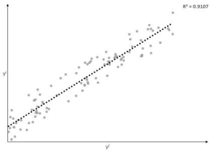
2.2 Structural relation between endogenous variable yj and exogenous variable yj0 . . . 88

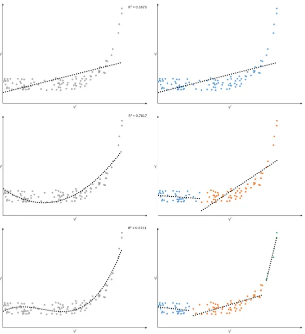
2.3 Linear Regression fit to nonlinear data . . . 90

2.4 Second Order Polynomial Function fit to nonlinear data . 90 2.5 Third Order Polynomial Function fit to nonlinear data . 91 2.6 Piecewise Approach to nonlinear data based on First, Second and Third Order Polynomial Function . . . 93

(16)

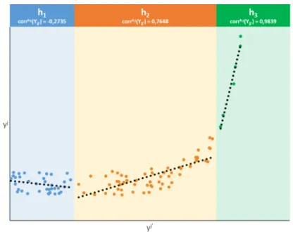
2.7 Piecewise Correlation built from a Third Order

Polyno-mial Function . . . 95

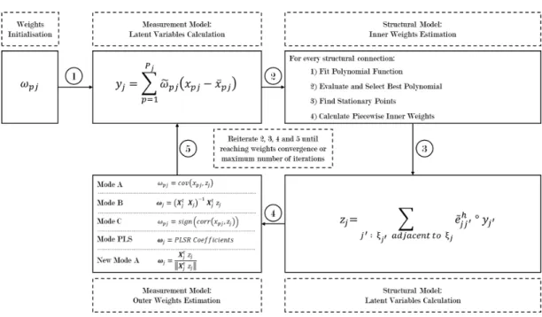
2.8 PLSPM Iterative Estimation Process using Piecewise In-ner Weights Estimation . . . 102

2.9 Nonlinear function jj0 output example . . . 104

2.10 Simulated Structural Equation Model . . . 105

2.11 Model Performance: Iterations to Convergence . . . 106

2.12 Measurement Model Comparison: Communality . . . 107

2.13 Measurement Model Comparison: Redundancy . . . 108

2.14 Structural Model Comparison: Latent Variables Statistics 109 3.1 Simulated Structural Equation Model . . . 113

3.2 Simulation Scenario 1: Distribution of Loading related to ⇠1 using the proposed algorithm . . . 118

3.3 Simulation Scenario 1: Distribution of Loading related to ⇠1 using the standard PLSPM . . . 119

3.4 Simulation Scenario 16: Distribution of Loading related to ⇠1 using the proposed algorithm . . . 120

3.5 Simulation Scenario 13: R2 Distribution Comparison: PLSPM vs. NL-PLSPM . . . 121

3.6 A non-convergence example: sample number 23 in Simu-lation Scenario 1 . . . 123

3.7 A non-convergence example: sample number 23 in Simu-lation Scenario 1 (last 50 iterations) . . . 123

(17)

4.1 Evolution of the Number of Customers in the Portuguese Energy Supply Market (Regulated and Liberalised)

be-tween 2006 and 2016 . . . 126

4.2 ECSI Model for EDPC: Structural Model . . . 130

4.3 EDP’s Input Data: Correlations between Manifest Vari-ables . . . 134

4.4 Unidimensionality Check: Principal Components . . . 137

4.5 Unidimensionality Check: Chronbach’s ↵ . . . 137

4.6 Unidimensionality Check: Dillon-Goldstein’s ⇢ . . . 138

4.7 Inner Model Summary: Perceived Value explained by Perceived Quality . . . 142

4.8 Inner Model Summary: Perceived Value explained by Ex-pectation . . . 144

4.9 Inner Model Summary: Perceived Quality explained by Expectation . . . 145

4.10 Inner Model Summary: Satisfaction explained by Expec-tation . . . 146

4.11 Inner Model Summary: Loyalty explained by Trust . . . 148

A.3.1 Simulation Scenario 1 - Loadings Estimates Distribution 210

(18)

A.4.1 Simulation Scenario 1 - R2 Distribution Comparison . . . 218

A.4.10 Simulation Scenario 10 - R2 Distribution Comparison . . 221

A.4.12 Simulation Scenario 12: R2 Distribution Comparison . . 222

A.5.1 Density Plot: Trustworthy company in what it says and what it does (Image 1) . . . 224

(19)

A.5.2 Density Plot: Stable and market-based company (Image 2)224

A.5.3 Density Plot: Company with a positive contribution to society (Image 3) . . . 225

A.5.4 Density Plot: Company that cares about customers (Im-age 4) . . . 225

A.5.5 Density Plot: Innovative and forward-looking company (Image 5) . . . 226

A.5.6 Density Plot: Overall expectations about the company (Expectations 1) . . . 226

A.5.7 Density Plot: Expectations about the company’s ability to o↵er products and services that meet customer needs (Expectations 2) . . . 227

A.5.8 Density Plot: Expectations regarding reliability, that is, how often things can go wrong (Expectations 3) . . . 227

A.5.9 Density Plot: Overall perceived quality (Perceived Qual-ity 1) . . . 228

A.5.10 Density Plot: Quality of electricity supply (Perceived Quality 2) . . . 228

A.5.11 Density Plot: Clarity and transparency in the informa-tion provided on safety, emergencies and consumpinforma-tion es-timates (Perceived Quality 3) . . . 229

A.5.12 Density Plot: Counselling and customer care (Perceived Quality 4) . . . 229

A.5.13 Density Plot: Billing and payment services’ reliability and quality (Perceived Quality 5) . . . 230

(20)

A.5.14 Density Plot: Accessibility via digital channels to the provided services (Perceived Quality 6) . . . 230

A.5.15 Density Plot: Stores and agents accessibility and avail-ability (Perceived Quality 7) . . . 231

A.5.16 Density Plot: Clarity and transparency in the informa-tion provided on contracting, billing and payment, com-plaints and commercial information (Perceived Quality 8) . . . 231

A.5.17 Density Plot: Products and services’ diversification (Per-ceived Quality 9) . . . 232

A.5.18 Density Plot: Evaluation of the price paid, given the qual-ity of products and services (Perceived Value 1) . . . 232

A.5.19 Density Plot: Evaluation of the quality of products and services, given the price paid (Perceived Value 2) . . . . 233

A.5.20 Density Plot: Overall satisfaction with the company (Sat-isfaction 1) . . . 233

A.5.21 Density Plot: Satisfaction compared to expectations (re-alization of expectations) (Satisfaction 2) . . . 234

A.5.22 Density Plot: Distance to the ideal electricity company (Satisfaction 3) . . . 234

A.5.23 Density Plot: Evaluation or Perceived evaluation of a complaint (Complaints 1) . . . 235

A.5.24 Density Plot: Overall trust (Trust 1) . . . 235

A.5.25 Density Plot: Confidence in Company’s performance (Trust 2) . . . 236

(21)

A.5.27 Density Plot: Intention to remain as a customer (Loyalty 1) . . . 237

A.5.28 Density Plot: Price sensitivity (Loyalty 2) . . . 237

A.5.29 Density Plot: Intention to recommend the company to colleagues and friends (Loyalty 3) . . . 238

A.7.1 Inner Model Summary: Expectation explained by Image 240

A.7.2 Inner Model Summary: Perceived Quality explained by Expectation . . . 240

A.7.3 Inner Model Summary: Perceived Value explained by Ex-pectation . . . 241

A.7.4 Inner Model Summary: Perceived Value explained by Perceived Quality . . . 241

A.7.5 Inner Model Summary: Satisfaction explained by Image . 242

A.7.6 Inner Model Summary: Satisfaction explained by Expec-tation . . . 242

A.7.7 Inner Model Summary: Satisfaction explained by Per-ceived Quality . . . 243

A.7.8 Inner Model Summary: Satisfaction explained by Per-ceived Value . . . 243

A.7.9 Inner Model Summary: Complaints explained by Satis-faction . . . 244

A.7.10 Inner Model Summary: Trust explained by Image . . . . 244

A.7.11 Inner Model Summary: Trust explained by Satisfaction . 245

A.7.12 Inner Model Summary: Trust explained by Complaints . 245

A.7.13 Inner Model Summary: Loyalty explained by Image . . . 246

(22)

A.7.15 Inner Model Summary: Loyalty explained by Complaints 247

(23)

1.1 Cronbach’s ↵ Assessment . . . 22

1.2 Convergence Scenarios for the PLSPM Algorithm (Henseler, 2010) . . . 41

2.1 An example of Dummy Encoding . . . 74

3.1 Simulation Scenarios . . . 115

3.2 Algorithm Convergence Analysis . . . 117

4.1 EDP’s Input Data: Summary Statistics for the Manifest Variables . . . 133

4.2 Outer Model Summary: Loadings, Communality and Re-dundancy . . . 140

3 Outer Model Summary: Cross-Loadings . . . 239

(24)

(25)

AVE CATI CCA ECSI EDP EDPC GME GoF GSCA GUI IPA LISREL LS LV LVPLS MIMIC ML MV NILES NIPALS OLS PCA PLS PLSPM PLS-R RGCCA SEM-ML TOL VIF

Average Variance Extracted

Computer-Assisted Telephone Interview Canonical Correlations Analysis

European Customer Satisfaction Index Energias de Portugal

EDP Comercial

Generalised Maximum Entropy Goodness of Fit

Generalised Structured Component Analysis Graphical User Interface

Importance-Performance Analysis LInear Structural RELations Least Squares

Latent Variable

Latent Variables Partial Least Squares Multiple Indicators for Multiple Causes Maximum Likelihood

Manifest Variable

Nonlinear Iterative LEast Squares

Nonlinear Iterative PArtial Least Squares Ordinary Least Squares

Principal Component Analysis Partial Least Squares

Partial Least Squares Path Modelling Partial Least Squares - Regression

Regularised Generalised Canonical Correlation Analysis Structural Equations Model - Maximum Likelihood Tolerance

(26)

(27)

All models are wrong, but some models are useful. George E.P. Box

Statistics researchers and business practitioners are constantly confronted with new challenges characterised by an ever-growing size and complex-ity.

Efron (2009) describes the current century as a period where the relation between data size and challenge complexity is characterised by large data sets and more sophisticated and targeted questions.

Hastie et al. (2009) explain that vast amounts of data are being gen-erated in many fields, and the statistician’s job is to make sense of it all: to extract important patterns and trends, and understand “what the data says”. The authors believe that the growing complexity associated to the process of “learning from data” have led to a revolution in the statistical sciences. Since computation plays such a key role, much of the new development has been done by researchers in other fields such as computer science and engineering. This “cross-pollination” made new

(28)

developments possible setting the foundations for a multidisciplinary re-search area: Computational Statistics, which is today a consolidated field aiming at analysing complex real phenomena using advanced computa-tional techniques.

The complexity of real phenomena is related to both the larger data set available and the amount of unknown influential factors present in real world. These changes in paradigm require the design of analyses that have to be customised and flexible, focussed on unveiling the real structure underlying the available data.

A real phenomenon can be analysed by identifying its main dimensions and defining a set of influential factors related to them. Scientific mod-elling aims at making a particular feature of the world easier to under-stand, define, quantify and visualise. As referred above, this process requires selecting and identifying relevant aspects of a situation in the real world and then applying di↵erent types of models based on the main goal; these models include conceptual models to better understand, op-erational models to opop-erationalise, mathematical models to quantify and graphical models to visualise the phenomenon under analysis.

However, when the analysed phenomenon presents sources of heterogene-ity, comes from several sub-populations or is influenced by other distur-bance factors, traditional methods often fail to recover the real structure underlying the data and more sophisticated procedures are required. This situation is no di↵erent for models like Partial Least Squares Path Modelling (PLSPM); this model aims at estimating the relationships among blocks of observable variables, which in turn are expression of latent (unobservable) variables.

(29)

The PLSPM algorithm is characterised by a system of interdependent equations based on simple and multiple linear regressions. The algorithm estimates the dependence relationships among latent variables (inner or structural model) as well as the relationships between manifest variables and their own latent variable (outer or measurement model). All the relations present in both inner and outer models are estimated under the assumption of linearity.

Although attractively simple, the traditional linear model often fails in some situations: in real life, e↵ects are often not linear (Hastie et al.,

2009).

The objective of this thesis is to propose a flexible data-driven alternative to the PLSPM algorithm tackling two main issues: (i) break the linearity assumptions present in the standard PLSPM algorithm; and (ii) accom-modate path direction within the inner model estimation phase through a non-symmetrical weighting estimation technique.

Thesis Outline Chapter 1 presents an historical overview of PLSPM

from its origins up to the latest developments; followed by theoretical analysis on measurement and structural models. Section 1.2.3 presents a state of the art on PLSPM algorithm and its extensions. The following section shows an overview on model validation techniques and comments the main issues related to the current assessment metrics. The chap-ter ends with a thorough study on open issues and sets the ground for the following chapters introducing the challenges related with linearity assumption and path direction incoherence.

(30)

in PLSPM and motivates the need for new developments focussed at answering the aforementioned questions. The subsequent sections show an overview on nonlinear modelling techniques and a detailed critical analysis on the available nonlinear approaches to PLSPM. Section 2.4

introduces and draws up the proposed approach, developed as part of this thesis; the final part of this section compares Nonlinear PLSPM results against the standard PLSPM model.

The algorithm presented in chapter 2 is tested for convergence and sta-bility in chapter 3. This chapter presents a wide Monte Carlo simulation analysis based on a comprehensive scenarios design phase. The results are then analysed and compared with the standard PLSPM algorithm. Chapter 4 presents an application focussed on a Customer Satisfaction study developed at EDP Comercial, one of the leaders in the Portuguese liberalised energy supply market. This application introduces a novel results interpretation tool provided by the proposed nonlinear approach to PLSPM.

The EQS code for the Monte Carlo simulated data and the R code for the nonlinear approach to PLSPM are provided in the appendix.

(31)

PLS Path Modelling

1.1 Historical Review

Partial Least Squares (PLS) methods made their first appearance in the 1960s when a research group at the Uppsala University, led by Herman Wold, developed the foundations of all modern PLS tools.

Herman Wold work was focussed on estimation methods for systems of simultaneous equations using least squares (LS) rather than Maximum-Likelihood (ML) (Mateos-Aparacio, 2011). His developments led him to a di↵erent estimation technique using iterative procedures, from which he created a new method called the Fixed-Point algorithm. This method uses an iterative ordinary least squares (OLS) algorithm to estimate the coefficients in a system of simultaneous equations (Wold, 1965).

Based on a comment received in 1964, during a conference on the Fixed-Point at the University of North Carolina, Wold steered the algorithm in order to calculate Principal Components (PCA) using an iterative

(32)

process (Fornell, 1982). Later developments led Wold to apply the al-gorithm for calculating Canonical Correlations (CCA) (Hotelling, 1936).

Fornell and Larcker (1987, p 408) define these approaches as belonging to a “second generation of multivariate analysis”.

The Fixed-Point algorithm, some years later, led him to his final do-main of interest: multivariate analysis and projection methods (Prin-cipal Components Analysis and its extension, PLS projection to latent structures) (Johnson and Kotz, 1998).

Herman Wold formalised the idea of partial least squares in his work on principal component analysis (Wold, 1966a,b) where the NILES al-gorithm, short for “Nonlinear Iterative LEast Squares”, was introduced. The latter paper presented a collage of examples solved by means of iterative procedures based on steps of least squares regressions.

Wold (1973) andNoonan and Wold(1977) works strengthen the founda-tions of PLS methods and renamed the category of methods from NILES to NIPALS (“Nonlinear Iterative PArtial Least Squares”). Given the fact that these first publications emphasised the iterative least squares approach to PCA, most authors refer to NIPALS as the PLS algorithm for PCA.

These first NIPALS procedures were never tagged as a single method-ology. On the contrary, they were seen as a collection of di↵erent algo-rithms for solving a diversity of methods such as PCA, CCA, regressions, and systems of econometric equations. The common goal of these pro-cedures was to linearise problems that were originally nonlinear in their parameters.

(33)

proce-dures. In fact, a Wold’s former Ph.D. student, Karl J¨oreskog, designed a novel approach to path modelling with latent variables based on ML estimation (i.e., models connecting two blocks of variables). Although Wold’s and J¨oreskog’s proposals present an approach to path modelling with latent variables, there are several di↵erences between the two ap-proaches (see Astrachan et al. (2014); Dolce (2015); Dolce and Lauro

(2015); Rigdon (2012, 2016); Vilares et al. (2010)).

J¨oreskog’s major accomplishments came from a multidisciplinary re-search that merged econometric simultaneous equations models, psycho-metric latent variable models, sociology causal analysis, and biopsycho-metric path analysis in a computer algorithm using the ML approach for pa-rameters estimation (J¨oreskog, 1970).

The combination of latent variables modelling and path models opened a whole new range of opportunities for researchers in the latent variables modelling area. Wold realised that some of the NIPALS procedures could be adapted for this new type of models.

In 1973, Wold re-branded again his methods from NIPALS procedures to NIPALS modelling with the intent of presenting NIPALS as a modelling framework (Wold, 1973). He positioned NIPALS modelling as “a design for the linearisation of models that are not linear in the parameters. The design is an ad hoc combination of (i) model specification in terms of causal and/or predictive relations, and (ii) parameters estimation”. That being said, NIPALS modelling was thus clearly reflecting a more mature but still incomplete modelling framework.

Still on the completeness of the NIPALS modelling framework, Joseph Kruskal once asked Wold “whether an explicit definition can be given

(34)

for the class of nonlinear models that constitute the scope of NIPALS modelling” (Wold, 1973). Wold answered that “NIPALS modelling is highly flexible, allowing the combined used of several devices, includ-ing parameter groupinclud-ing and relaxation; auxiliary transformation of the model; and modelling the predictors in terms of indirectly observed man-ifest variables and other hypothetical constructs”, identifying “NIPALS modelling as an open ended array of models with unlimited complexity in the combined use of several devices”.

In mid-1970s, Wold and his team at the University of G¨oteborg refined and published several versions of a common methodology to estimate path models by using an iterative algorithm of least squares regressions. It is worth mentioning: (i) an extension of the algorithm that allows handling three blocks (as opposed to the previous two blocks algorithm); and (ii) the extension of handling more than one between-block relation (Wold, 1974, 1975a,b).

During the same period Wold encased his modelling framework based on the PLS approach under the “Soft Modelling” insignia (Wold, 1975b). The NIPALS approach is applied to the “soft” type of model used in social sciences in the last years, specifically path models a↵ecting latent variables which serve as proxies for blocks of indirectly observed variables. “Soft modelling” implies the idea of modelling in “complex situations where data and prior information are relatively scarce and without spec-ifying assumptions about the stochastic-distributional properties of vari-ables and residuals” (Wold, 1975b).

Johnson and Kotz (1998) describes Herman Wold as “a very practical man, and wanted estimation and modelling methods to work with a

(35)

minimum of assumptions, for incomplete data, with many variables and collinear variables, etc.; and he developed PLS accordingly”. This practi-cality is confirmed in “Path Models with Latent Variables: The NIPALS Approach” (Wold, 1975a), where Wold states that sometimes “the model builder has little or no more prior information at disposal for the model construction than its intended operative use. The NIPALS models are designed with particular view to applications in such low-information situations”.

After several adjustments made during the 1970s, Wold and his team ar-rive to a more defined framework and the acronym NIPALS is shortened to PLS. The end of the 1970s decade sees the official presentation of the so-called Basic Design for PLS path modelling.

The Basic Design represents the basic method for PLS Path Analy-sis with Latent Variables and it has been firstly published in “Causal-Predictive Analysis of Problems with High Complexity and Low Informa-tion: Recent Developments of Soft Modelling” and then in Wold (1980). This method represents the main reference on top of which all extensions and modifications are based on. More theoretical details can be found in

Wold (1982a,b,c) and a practical application to the chemometric area is provided inGerlach et al.(1979). Geometric interpretations are provided by Fred Bookstein (Bookstein, 1980, 1982).

Also in 1979, Karl J¨oreskog and Herman Wold organised a meeting that brought together the LISREL1 (or SEM-ML community) and PLS

com-1_{LISREL (LInear Structural RELations) is the “informal” name that the}

commu-nity gave to the ML approach to Structural Equations Modelling published by Jöreskog in Jöreskog(1970). The term LISREL was the name given to the implemented soft-ware (Jöreskog and Sorbom,1993). However, it had such a rapid development that the

(36)

munity generating interesting contents then published in the form of the classic two-volume book: “Systems under indirect observation: Causal-ity, structure, prediction”.

In 1989, Jan-Bernd Lohmöller published the book “Latent Variable Path Modeling with Partial Least Squares” (Lohmöller, 1989) where he pre-sented the basic PLS Path Modelling (PLSPM) algorithm and his ex-tended version. For many years LVPLS 1.8 (developed by Lohmöller,

1984) was the unique available software on PLS Path Modelling. What is perhaps the first pseudo-code description of the basic algorithm is also provided in Lohm¨oller (1989) (p. 29).

As mentioned in the previous paragraph, Lohm¨oller extended the basic PLS algorithm in various directions. More details can be found in section

1.2.

Strangely enough, during the 1990s, the theoretical developments on PLS Path Modelling slowed down dramatically. One of the most interesting work was presented on the computational side with the development of PLS-Graph by Wynne Chin (Chin, 1998b).

The beginning of the XXI century saw a renewed interest in PLSPM and major contributions were made. The main reference in this pe-riod was the paper “PLS path modeling” by Tenenhaus, Esposito Vinzi, Chatelin, and Lauro (2005). Other relevant authors in this field are Ringle, Henseler and Dijkstra.

In 2005 a new software was made available by Ringle et al. (2005b) and their work has been an on-going process with a series of versions (the current one being SmartPLS 3).

(37)

On the theoretical side, Hanafi (2007) and Tenenhaus and Hanafi (2010) presented two fundamental works that aimed at better understanding the PLSPM algorithm. They developed extensions to the multi-block approach initiated by Lohm¨oller and Hanafi has resolved some of the issues around the convergence of the PLSPM algorithm. An interesting work on the convergence issue has been provided by Kr¨amer (2007). Its findings will be presented with more detail in section 1.3.

Other alternative approaches to PLSPM have been proposed. Namely, the Generalised Maximum Entropy (GME) presented byAl-Nasser(2003) and the Generalised Structured Component Analysis (GSCA) by Hwang and Takane (2004).

Two interesting reviews on PLS path modelling empirical applications can be found in Marcoulides et al. (2009) and Ringle et al. (2012). More recently, Tenenhaus and Tenenhaus (2011) proposed the Regu-larised Generalised Canonical Correlation Analysis (RGCCA), a new modification to the PLSPM algorithm in such a way that convergence is guaranteed; additionally, PLS Regression2 is presented as one of its special cases. This approach represents a generalisation of regularised canonical correlation analysis to three or more sets of variables. It con-stitutes a general framework for many multi-block data analysis methods and combines the power of multi-block data analysis methods, such as the maximisation of well identified criteria, and the flexibility of PLS path modelling. The big achievement is the fact that this paper, extend-ing Hanafi (2007) work on convergence, presents a new monotonically

2_{PLS Regression (PLS-R) (}_Tenenhaus_,₁₉₉₈_;_{Wold et al.}_,₁₉₈₃_{) represents a slightly}

modified PLSPM algorithm with the objective of obtaining a regularised component based regression toolTenenhaus (1998); Wold et al. (1983).

(38)

convergent algorithm very similar to the PLS algorithm proposed by Herman Wold. This new proposal achieves convergence introducing a modified Mode A in which the outer weights are normalised to unitary variance at each step of the algorithm. Contrary to classical Mode A, this new estimation mode has the major advantage to maximise a known criterion.

During the last year, a set of papers discussed the di↵erences between the SEM-ML approach and the PLS approach to Structural Equation Mod-elling. The review papers by Rigdon (2012) and Ronkko and Evermann

(2013) started two interesting and active discussion streams.

The first critical review published by Rigdon in 2002 (Rigdon, 2012) states that PLS path modelling “has strengths as a tool for prediction which have not been fully appreciated” and “can move forward by freeing itself entirely of its heritage as ‘something like but not quite factor anal-ysis’, by fleshing out inferential tools appropriate for a purely composite method and by developing approaches for assessing measurement valid-ity that properly recognise the distinction between theoretical concepts and empirical proxy”.

The paper published by Sarstedt, Ringle, Henseler, and Hair(2014) criti-cises the comments made by Rigdon in the aforementioned review, giving “their version of the truth” focussing mainly on prediction, explanation and model assessment. The authors clarify that there should not be a dichotomy between predictive and explanatory modelling and that PLS path modelling (referred as PLS-SEM in their paper) should not be forced to “choose a side”.

(39)

the PLS genesis and focussing on two main topics: (i) suitability of PLS path modelling as a tool for estimating structural relationships; and (ii) whether the factor scores produced by PLS path modelling can be deter-mined unambiguously or they should be obtained by using composites instead. Other critics to Rigdon’s strong statements are presented in

Bentler and Huang (2014).

This sequence of comments ends, at least for now, with a “closing” and clarifying paper presented by Rigdon (2014). The author tries to answer all the comments and flaws highlighted in the previous reviews. Rigdon subdivides the challenges in nine main arguments described in his work. In addition to the previous paper, Rigdon (2016) published a thorough analysis on the practical use of PLS path modelling identifying: (i) flaws related to invalid arguments in favour of using PLSPM; and (ii) invalid arguments opposing its use within the context of a unifying framework to be used as an analytical method in European management research. Other authors focussed on developing a unified framework are Sarst-edt et al. (2016). The authors validated their conceptual considerations based on a simulation study, highlighting the biases that occur when us-ing (i) composite-based partial least squares path modellus-ing to estimate common factor models, and (ii) common factor-based covariance-based structural equation modelling to estimate composite models. Their re-sults show that the use of PLSPM is preferable, particularly when it is un-known whether the data’s nature is common factor-based or composite-based.

Ronkko and Evermann (2013) presented a review on the application and applicability side of PLS path modelling. This paper strongly criticises

(40)

PLS path modelling suitability for di↵erent applications and presents the authors’ doubts regarding its e↵ectiveness in building and testing theory in organisational research. This review generated a detailed answer from

Henseler et al. (2014) who pointed out that “the shortcomings of PLS are not due to problems with the technique, but instead to three prob-lems with Ronkko and Evermann (2013) study: (i) the adherence to the common factor model; (ii) a very limited simulation design; and (iii) over-stretched generalisations of their findings”.

The result of such a rich amount of ideas and views allows us to get a deeper view on PLS path modelling capability and suitability in di↵erent situations and application areas.

More recently, a group of researchers shifted their focus on PLSPM pre-diction capabilities. Shmueli et al. (2016) stated that, so far, PLSPM literature has not made a full use of these predictive proprieties, using instead an explanatory approach focussed on statistical significance and power (Becker et al.,2013). Shmueli and Koppius(2010,2011) reinforced the previous statements saying that quantitative research in management has been dominated by causal-explanatory statistical modelling at the expense of predictive modelling. More details on this topic are presented in section 1.2.5.

Our position with regards to the aforementioned papers is that PLS path modelling is often discussed and used as if it was a kind of factor analysis but, as mathematically shown by Rigdon, it is a purely composite-based method. Also, the fact that PLS path modelling represents a better model for prediction does not imply that the same cannot be used for explanatory analysis. The PLS path modelling community needs to

(41)

em-brace the method’s character as a composite-based method; this requires shedding the factor-based jargon, perspectives, evaluation tools and mea-surement framework of factor-based SEM and developing alternatives. Another important set of opportunities is related to the predictive as-sessment of PLSPM. The latest steps toward prediction-driven PLSPM applications and the formalisation of a predictive assessment framework are widening the possibilities associated to the use of PLSPM.

The next sections present the original algorithm by Herman Wold, its extensions and open issues.

1.2 PLS Path Modelling

As discussed in the previous sections, PLS path modelling can be de-scribed as a composite-based estimation method which aims at analysing the complexity existent in a specific system by estimating the causal rela-tions between latent variables (LVs) defined as components or composites and measured by a set of manifest variables (MVs).

Formalising the previous concepts, PLS path modelling focusses on study-ing the relationships among J blocks X1, . . . , Xj, . . . , XJ of MVs,

which represent J latent variables ⇠1, . . . ,⇠j, . . . ,⇠J, defined as

com-posites.

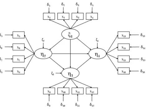
PLSPM adhere to a specific graphical convention (see Figure 1.1) based on the drawing principles defined in the path analysis (Wright, 1921,

1934). More in detail, ellipses or circles represent the latent variables, and rectangles or squares refer to manifest variables, whereas unidirectional arrows are used to relate MVs with LVs and also causations among LVs.

(42)

Figure 1.1: PLSPM Graphical Notation

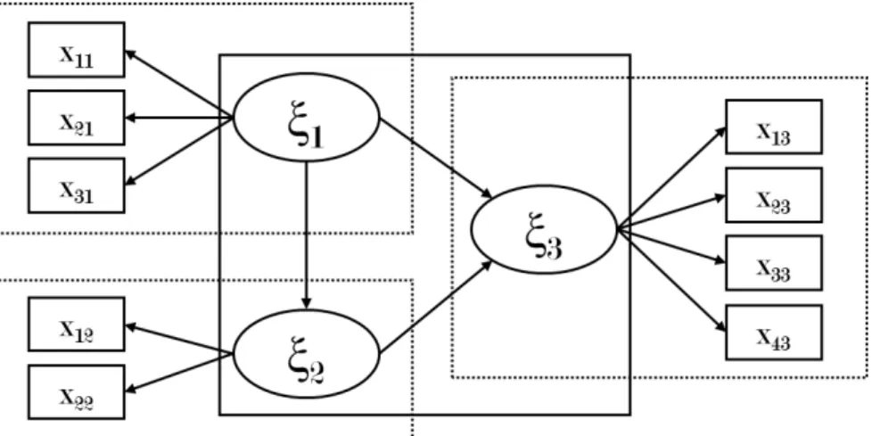
A PLS path model (see Figure 1.2) is made up of two elements: (i) the measurement model (or outer model) which describes the relationships between the MVs and their respective LVs; and (ii) the structural model (or inner model) which describes the relationships between the LVs. Both models are described in the next sections.

(43)

1.2.1 The Measurement Model

A LV ⇠j is an unobservable variable (also named composite or construct)

indirectly described by a block of observable variables Xj which are

called MVs or indicators. There are several ways to relate the MVs to their LVs:

– The reflective way (or outwards directed way); – The formative way (or inwards directed way);

– The MIMIC way (a combination of both reflective and formative).

Reflective Way

In the reflective way each MV reflects the corresponding LV (see Figure

1.3). A block is defined as reflective if the LV is assumed to be a common factor that reflects itself in its respective MVs.

Figure 1.3: Measurement Model: the Reflective Way

In this model each MV is related with its LV by a simple linear regression.

(44)

where ⇠j has mean m and standard deviation equal to 1.

The model defined in equation 1.1 has to follow only one hypothesis named predictor specification and defined by H. Wold in his seminal papers:

E(xpj|⇠j) =⇡p0+⇡pj⇠j (1.2)

This hypothesis implies that the residual ✏p has a zero mean and is

un-correlated with the LV ⇠j.

In the reflective model each block of MVs Xj, has to be unidimensional

in the sense of factor analysis. The ultimate goal is that all the MVs belonging to one block have to present a strong correlation.

When working with real data and using a reflective model, it is very important to check the unidimensionality for each block of MVs.

There are three main techniques used to check the unidimensionality: – Principal Component Analysis: a block can be considered

unidi-mensional if the first eigenvalue of the correlation matrix, built based on all the MVs related to the block, is greater than 1 and the second one smaller than 1, or at least far enough from the first one. After checking the eigenvalues, it is important to verify that all the MVs are positively correlated with the first factor (in the sense of PCA). A MV becomes inadequate to measure the LV when its correlation with the first factor is negative.

– Cronbach’s ↵: this statistic can be used to check unidimensionality in a block of Pj manifest variables Xj, when they are all

(45)

posi-tively correlated. Cronbach proposed the following procedure for standardised variables:

The variance of PPj_p₌₁xpj is developed as follows:

V ar 0 @ Pj X p=1 xpj 1 A=Pj + X p₆=p0 corr⇣xpj, x_p0_j ⌘ (1.3)

The larger P_p₆₌_p0 corr

⇣

xpj, x_p0_j

⌘

the more the block Xj is

unidi-mensional.

Based on equation 1.3 is possible to calculate the following ratio:

↵0 = P p6=p0 corr ⇣ xpj, x_p0_j ⌘ Pj +P_p₆₌_p0 corr ⇣ xpj, x_p0_j ⌘ (1.4)

When all correlations corr⇣xpj, x_p0_j

⌘

are equal to 1, ↵0 reaches its maximum value, i.e., (Pj 1)Pj.

The maximum value is then used to obtain the Cronbach’s ↵ di-viding ↵0 by its maximum value:

↵ = P p6=p0 corr ⇣ xpj, x_p0_j ⌘ Pj +P_p₆₌_p0 corr ⇣ xpj, x_p0_j ⌘ ⇥ _PPj j 1 (1.5)

When working with the original manifest variables (non-standardised), Cronbach’s ↵ is calculated as follows:

↵ = P p₆=p0 corr ⇣ xpj, x_p0_j ⌘ V ar⇣PPj p=1xpj ⌘ ⇥ _PPj j 1 (1.6)

(46)

The following table (Cortina, 1993) can help assessing ↵’s values:

Cronbach’s ↵ Internal Consistency

↵ 0.9 Excellent 0.9> ↵ 0.8 Good 0.8> ↵ 0.7 Acceptable 0.7> ↵ 0.6 Questionable 0.6> ↵ 0.5 Poor 0.5> ↵ Unacceptable

Table 1.1: Cronbach’s ↵ Assessment

In accordance with (Cortina, 1993) a block can be considered uni-dimensional when ↵ is larger than 0.7.

– Dillon-Goldstein’s ⇢: by construction, the correlation signs between manifest variablesxpj and the latent variable⇠j have to be positive,

that is, in the equation 1.1 all loadings ⇡pj are positive. A block

can be defined unidimensional when all loadings are large. The first step is represented by defining the variance of PPj

p=1xpj. For this specific case the variance is calculated from equation 1.1

(47)

V ar 0 @ Pj X p=1 xpj 1 A =V ar 0 @ Pj X p=1 (⇡p0+⇡pj⇠j +✏p) 1 A = 0 @ Pj X p=1 ⇡pj 1 A 2 V ar(⇠j) + Pj X p=1 V ar(✏p) (1.7) The larger ⇣PPj p=1⇡pj ⌘2

the more the block Xj is unidimensional.

The Dillon-Goldstein’s ⇢ is defined as:

⇢ = ⇣PPj p=1⇡pj ⌘2 V ar(⇠j) ⇣PPj p=1⇡pj ⌘2 V ar(⇠j) +PP_p₌₁j V ar(✏p) (1.8)

In an initial stage, the values of⇠j are not available and an

approx-imation is needed. Based on the assumption that all MVs xpj and

the LV ⇠j are standardised, it is possible to obtain a LV

approx-imation using the first factor t1 from a PCA on all MVs related with the block.

The loading ⇡pj can be estimated by corr(xpj, t1) and, based on equation 1.1, the a V ar(✏p) is estimated by 1 corr2(xpj, t1).

The estimated Dillon-Goldstein’s ⇢ can be calculated as:

ˆ ⇢= hPPj p=1corr(xpj, t1) i2 hPPj p=1corr(xpj, t1) i2 +PPj p=1[1 corr2(xpj, t1)] (1.9)

(48)

A block can be considered unidimensional when ˆ⇢ is larger than 0.7.

This statistics is considered to be a better option to check unidi-mensionality for a block of manifest variables (Chin, 1998a).

Formative Way

In a formative model the latent variable ⇠j is obtained through a

lin-ear combination of the related manifest variables (see Figure 1.4) and a residual term: ⇠j = Pj X p=1 !pjxpj + j (1.10)

Using this measurement model scheme, unidimensionality of the block is not required (i.e., a block of manifest variables is allowed to be multidi-mensional).

Figure 1.4: Measurement Model: the Formative Way

The hypothesis related to the predictor specification for the equation

(49)

E ⇠j|x1, . . . , xPj = Pj

X

p=1

!pjxpj (1.11)

This hypothesis implies that the residuals j has mean 0 and is not

correlated with the manifest variables xpj.

In this scheme the LV is generated from a linear combination of its MVs and there is no sign constraints on the weights !pj, but unexpected signs

show problems in data that might be related to multicollinearity. If the model’s results present unexpected signs the user can remove the MV from input data or, as shown inTenenhaus, Esposito Vinzi, Chatelin, and Lauro (2005), sign constraints can be easily added to the PLS algorithm.

MIMIC (Multiple Indicators for Multiple Causes)

In a MIMIC scheme the latent variables are seen as a mix of formative and reflective relationships. The measurement model for a specific block

Xj is defined as follows.

Let PR represent the set of MVs following the reflective scheme,

when the arrows are outward directed (reflective scheme) the simple re-gression on xpj can be written as:

xpj = ⇡p0+⇡pj⇠j +✏p for p2PR (1.12)

when the MVs are inward directed (formative scheme), the latent variable

⇠j can be determined as:

⇠j =

X

p /2PR

(50)

The predictor specification hypothesis for equations 1.12 and 1.13 are the same mentioned in the previous sections.

Thoughts on Measurement Model’s Schemes

The previous paragraphs presented three measurement model schemes related, in some way, to the assumed directions of the connections be-tween manifest and latent variables.

The “reflective” measurement scheme is used to describe an outer model where manifest variables act as dependent upon an unmeasured variable. Reverting the direction of the outer relation, the unobserved variable is modelled as dependent from the manifest variables; this scheme is known as “formative”. A mixture of inward and outward directed connection belonging to the same block corresponds to the MIMIC scheme.

It is important to separate the conceptual analysis of these measurement schemes from the technique used to calculate the latent variables proxies (or composites).

The PLS path modelling presents several options to calculate the latent variables proxies; the most known techniques are “Mode A” and “Mode B” (explained in detail throughout this chapter). For years Mode A and Mode B have been associated to reflective and formative schemes, respec-tively. As Rigdon (2016) strongly affirms, “this is an illusion”. In fact, both modes create composites and the only di↵erence standing between the two is the way how weights are obtained (using Mode A instead of Mode B means using correlation weights instead of OLS regression coefficients).

(51)

collinearity among predictors. This di↵erence represents an advantage for the users that prefer correlation weights because this technique does not experience unexpected weights signs driven by collinearity.

As confirmed by Becker et al. (2013) for PLS path modelling, Dana and Dawes (2004) demonstrated that, while correlation weights yield a somewhat lower in-sample R2 than OLS regression weights, they yield a higher out-of-sample R2 when sample size and true predictability are moderate, potentially covering a much larger range of practice than the special conditions required for OLS regression weights to stand out. There can be good reasons to choose Mode A or Mode B within a PLS path modelling; this choice has nothing to do with the conceptual scheme idealised for the measurement model (choice between “formative” and “reflective”).

The real choices a researcher faces whilst implementing a PLS path model are between common factor proxies and composite proxies, and between regression weighted composites and correlation weighted composites. In summary, this work shares Rigdon’s position on this matter: “the the terms formative and reflective only obscure the statistical reality” (Rigdon, 2016).

The MIMIC conceptual scheme is difficult to implement within a PLSPM context (Fornell and Bookstein, 1982), but the problem may be faced by splitting the MIMIC variable into two blocks of manifest variables (an endogenous and an exogenous one) with a known relationship between original and new path coefficients.

(52)

1.2.2 The Structural Model

The causal model shown in figure 1.2 presents three latent variables con-nected by a causal relationship. These relationships build the structural model (or inner model) and can be formalised as follows:

⇠j = j0+

X

j₆=j0

jj0⇠j0 +⌫j (1.14)

The predictor specification hypothesis also applies for equation 1.14. A latent variable which never appears as dependent in equation 1.14 is known as exogenous variable. The other LVs are defined as endogenous variables.

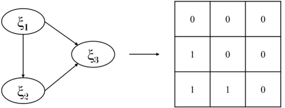
The causality model must be a causal chain. That means that there is no loop in the model. This kind of model is called recursive, from the Latin Recursio, which means I can return (Tenenhaus et al., 2005). Every structural model can be described through a square matrix con-taining binary values (see Figure 1.5). Its dimension is equal to the number of latent variables J. Lohm¨oller defines this matrix as inner design matrix (Lohm¨oller, 1989).

(53)

Let l and k be respectively rows and columns indexes of the aforemen-tioned matrix, cell (l, k) has value of 1 when latent variable ⇠k causes ⇠l;

0 otherwise.

The structural model estimation process is shown in the next sections.

1.2.3 Algorithm: State of the Art

PLS path modelling has been firstly developed byWold(1975b). Lohm¨oller

(1989) presented new theoretical and computational developments (LV-PLS software). A first software with graphical interface ((LV-PLS-Graph) has been developed by Chin (1998a,b). PLS-Graph is based on Lohm¨oller’s proposed algorithm presenting some new and improved validation tech-niques.

The current work is based on the algorithm proposed byLohm¨oller(1989) which is described in the next paragraphs.

As discussed in the previous sections, PLS path modelling aims to esti-mate relationships among J (j = 1, . . . , J) blocks of variables, which are expression of unobservable constructs. The algorithm is composed by a system of interdependent equations based on simple and multiple linear regressions. The algorithm estimates the causal e↵ects among LVs as well as the relationships between MVs and their own LVs.

(54)

Starting Weights Definition

The first step of the PLSPM algorithm regards the definition of a set of arbitrary weights wpj to be used as starting point. The weights are then

normalised in order to produce LVs with unitary variance.

There are several ways to define the starting weights. One of the most common choices is wpj = sign[corr(xpj,⇠j)]; this is applied in practice

by setting wpj =sign[corr(xpj,⇠j)] when p= 1 and 0 otherwise.

As of today, the starting weights choice does not seem to interfere with the final results but it does have an impact on how quickly the algorithm reaches convergence.

Measurement Model: Latent Variables Calculation

Once defined the initial weights the algorithm moves to the outer estimate

yj of the standardised (with mean = 0 and standard deviation = 1) latent

variables (⇠j mj). The composites are calculated as linear combination

of their centered MVs: yj _/_± 2 4 Pj X p=1 wpj(xpj xpj¯ ) 3 5 (1.15)

where the _/ symbol means that the variables on the left is proportional to the operator on the right; the _± sign represents the sign ambiguity. This problem is solved by selecting the sign that makes the variable yj

positively correlated with the majority of manifest variables xpj.

(55)

yj = Pj X p=1 ˜ wpj(xpj xpj¯ ) (1.16)

The coefficients wpj and ˜wpj are called outer weights.

The mean value mj is estimated as:

ˆ mj = Pj X p=1 ˜ wpjx¯pj (1.17)

and the latent variable ⇠j is estimated by:

ˆ ⇠j = Pj X p=1 ˜ wpjxpj = yj + ˆmj (1.18)

Structural Model: Inner Weights Estimation

The structural model aims to give an estimate of the LVs based on the causal relations present in the inner model. The inner weights e_jj0 can

be estimated through several techniques.

Centroid Scheme The centroid scheme represents the original

tech-nique proposed by H. Wold and is also one of the most used techtech-niques to estimates inner weights. Following this technique e_jj0 can be obtained

as: e_jj0 =sign h corr⇣yj, y_j0 ⌘i (1.19) In this case e_jj0 are expressed as the correlation sign between y_j and the

(56)

connected if they are linked in the structural model (i.e., an arrow goes from one variable to the other describing their causality relation).

The centroid scheme presents some inconvenience when correlations be-tween LVs are very close to 0. In fact, when this situation happens, corre-lations fluctuate between positive and negative values creating apparent instability. Tenenhaus, Esposito Vinzi, Chatelin, and Lauro(2005) state that this choice does not seem to be a problem in practical applications.

Factorial Scheme The Factorial Scheme is one of the two

tech-niques proposed by Lohm¨oller where inner weights e_jj0 are calculated as

follows: e_jj0 = r_jj0 =corr ⇣ yj, y_j0 ⌘ (1.20) By choosing this technique, the inner weights correspond to the cor-relation between latent variables. According to Lohm¨oller (1989), this technique should solve the drawbacks presented by the Centroid Scheme. Even though this new scheme do not significantly influence the results, it is very important for theoretical reasons. In fact, as shown in Tenenhaus, Esposito Vinzi, Chatelin, and Lauro (2005), it allows to relate PLS path modelling to usual multiple table analysis methods.

Path Weighting (or Structural) Scheme The Path Weighting

Scheme is the second technique proposed by Lohm¨oller. The LVs con-nected to ⇠j are divided into two groups: the predecessors of ⇠j which

are LVs explaining ⇠j, and the followers which are LVs explained by ⇠j.

(57)

regression coefficient ofy_j0 in the multiple regression ofyj on all the y_j0’s

related to the predecessors of ⇠j. If ⇠_j0 is a successor of ⇠j then the inner

weight e_jj0 is equal to the correlation between y_j0 and y_j.

Summarising, when using the Path Weighting scheme, inner weights e_jj0

are calculated as:

e_jj0 = regression coefficient of y_j on all y_j0 if ⇠_j0 explains ⇠_j

= r_jj0 if ⇠j explains ⇠_j0

(1.21)

The Path Weighting Scheme represents the only scheme where the di-rection of structural relations is taken into account (Dolce, 2015). As referred for the Factorial Scheme, this technique also allows to relate PLS path modelling to usual multiple table analysis methods.

Structural Model: Latent Variables Calculation

In the inner LVs calculation stage, the standardised (⇠j mj) latent

variables inner estimation zj is given by:

zj /

X

j0 : ⇠

j0 adjacent to ⇠j

e_jj0 y_j0 (1.22)

where denotes the Hadamard product.

Measurement Model: Outer Weights Estimation

There are several ways to estimate the outer weights wjh. Originally, H.

(58)

(Wold, 1975b). Later on, Lohm¨oller proposed a third technique: Mode C (Lohm¨oller, 1989). More recently, two more techniques have been proposed: Mode PLS (Esposito Vinzi, 2008, 2009; Esposito Vinzi and Russolillo, 2013) and New Mode A (Tenenhaus and Tenenhaus, 2011).

Mode A Each outer weight wpj is the regression coefficient in the

simple linear regression of the p-th MV xpj, belonging to the j-th block Xj, on the composite zj of the j-th LV. As a matter of fact, as zj is

standardised, the generic outer weight wpj is represented by the

regres-sion coefficient associated to zj in the simple linear regression of xpj on

zj. In more detail:

wpj =cov(xpj, zj) (1.23)

where, as referred above, the estimated latent variable zj is standardised.

Mode B In mode B, the outer vectorwj of weightswpj is composed

by the regression coefficient vector in the multiple regression of zj on the centered manifest variables (xpj x¯pj) related to the same latent variable

⇠j:

wj = XtjXj 1Xtjzj (1.24)

where Xj is a matrix having on the columns the centered manifest

vari-ables (xpj x¯pj) related with the same latent variable ⇠j.

Mode C Lohm¨oller added a new mode C for the calculation of the

(59)

absolute value and reflect the signs of the correlations between the MVs and their LVs:

wpj =sign(corr(xpj, zj)) (1.25)

These weights are then normalised so that the resulting LV has unitary variance. Mode C actually refers to a formative way of linking MVs to their LVs and represents a specific case of mode B whose comprehension is very intuitive to practitioners.

Mode PLS In order to solve the problems related with

multi-collinearity a new way to compute outer weights, in the case of a forma-tive block, has been recently proposed by Esposito Vinzi (2008, 2009);

Esposito Vinzi and Russolillo (2013). This approach involves using PLS Regression (PLS-R) (Tenenhaus, 1998; Wold et al., 1983) in order to compute significant outer weights. In particular, Esposito Vinzi (2009) proposes to calculate at each iteration the outer weights as coefficients in a PLS Regression of the LV inner composite on the MVs linked to the same LV. PLS-R method has been extensively described in literature (Tenenhaus, 1998; Wold et al., 1983). PLS-R is a linear regression tech-nique that allows relating a set of predictor variables to one or several response variables. PLS-R shrinks the predictor matrix by sequentially extracting orthogonal components which, at the same time, summarise the explanatory variables and allow modelling and predicting the re-sponse variables. Finally, it provides a classical regression equation, in which the response is estimated as a linear combination of the predictor

(60)

variables.

New Mode A Traditional Mode A applied to all the blocks does

not seem to optimise any criterion; as Kr¨amer (2007) showed, Wold’s Mode A technique does not lead to a stationary equation related to the optimisation of a twice di↵erentiable function. However, Tenenhaus and Tenenhaus (2011) recently extended the results of Hanafi (Hanafi, 2007) to a slightly adjusted Mode A in which a normalisation constraint is placed on outer weights rather than on LV composites. In particular, they showed that Wold’s procedure, applied to a PLS path model where the new Mode A is used in all the blocks, monotonically converges to the following criterion: arg max ||wj||2=||w_j0||2=1 X j₆=j0 c_jj0g ⇣ cov⇣Xjwj,X_j0w_j0 ⌘⌘ (1.26)

where g is defined as:

g(x) = 8 > < > : x2 if factorial |x_| if centroid (1.27)

In the new mode A, the outer vector wj of weights wpj is

wj =

Xt_jzj ||Xt_jzj||

(1.28) We may note that the outer composite yj = Xjaj is the first PLS

com-ponent in the PLS regression (Tenenhaus, 1998; Wold et al., 1983) of the inner composite zj on block Xj. In the original mode A of the PLS

(61)

approach, the outer weights are computed in the same way as formula

1.23 but normalised so that the outer component yj = Xjaj is stan-dardised. This new mode A shrinks the intra-block covariance matrix to the identity. This shrinkage is probably too strong, but is useful for very high-dimensional data because it avoids the inversion of the intra-block covariance matrix.

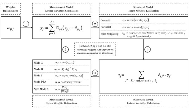
Iterative Process and Convergence

After the first cycle the algorithm iterates the following steps: 1. Measurement Model: Latent Variables Calculation 2. Structural Model: Inner Weights Estimation

3. Structural Model: Latent Variables Calculation 4. Measurement Model: Outer Weights Estimation 5. Outer Weights Convergence Check

The aforementioned algorithm is described in figure 1.6 and its pseudo-code is shown in Algorithm 1.

After reaching the algorithm convergence, the outer weights wjh are used

to obtain the final estimation of ⇠j calculated as ˆ⇠j =Pwjhxjh.

In the last step of PLSPM algorithm, path coefficients are estimated through an OLS multiple regression among the estimated latent vari-ables composites, according to path diagram structure. Denoting ⇠j

(62)

Figure 1.6: PLSPM Iterative Estimation Process

of the corresponding latent predictors, the path coefficient vector j for

each ⇠j is obtained as:

j =

⇣

⌅0_!_j⌅_!j

⌘ 1

⌅0_!_j⇠ˆj (1.29)

Algorithm Convergence As previously mentioned, PLS path

mod-elling is mostly used to analyse complex relationships among latent vari-ables.

Many fields of research have embraced the specific advantages of PLSPM, behavioural sciences for instance (Bass et al., 2003) as well as many disciplines of business research such as marketing (Anderson et al., 1994;

Fornell and Larcker, 1987; Matzler et al., 2004) and many others. The PLSPM advantages highlighted in these papers are confirmed in practice by its wide adoption in many organisations.

(63)

Algorithm 1: PLS Path Modelling (Lohm¨oller’s Algorithm)

Input : X = [X1, . . . ,Xj, . . . ,XJ]

Output: wpj,⇠ˆj, j

1 Arbitrary Weights Initialisation: w_pj =w_pj(0)

2 while Convergence of wpj is not reached (or max number of

iterations) do

3 Latent Variables Composites Calculation (Measurement

Model):

yj / ±[Pwpj(xpj x¯pj)]

4 Inner Weights Estimation (Structural Model):

e_jj0 = f

⇣

yj, y_j0

⌘

according to the chosen scheme

5 Latent Variables Composites Calculation (Structural

Model): zj /P_j0 _: _⇠ j0 adjacent to ⇠j ⇣ e_jj0 y_j0 ⌘

6 Outer Weights Estimation (Measurement Model):

wpj = f(X,Z) according to the chosen estimation technique

7 Final Latent Variables Composites Calculation:

ˆ

⇠j = Pwpjxpj

8 Path Coefficients Calculation:

j =

⇣

⌅0_!_j⌅_!j

⌘ 1

⌅0_!_j⇠ˆj

Henseler (2010) in his paper states that the popularity of PLSPM among scientists and practitioners results from four genuine advantages:

– Can be used when distributions are highly skewed (Bagozzi and Yi,

1994), because “there are no distributional requirements” (Fornell and Bookstein, 1982);

– Can be used to estimate relationships between latent variables with several indicators when sample size is small (Chin and Newsted,

(64)

– Availability of modern and easy-to-use software with graphical user-interface, like SmartPLS (Ringle et al.,2005b) and PLS-Graph (Chin, 1998b), have contributed to increase the attractiveness of PLSPM;

– PLSPM is preferred over covariance-based structural equation mod-elling when improper or non-convergent results are likely, as for instance in more complex models, when the number of latent and manifest variables is high in relation to the number of observations and the number of indicators per latent variable is low.

Notwithstanding the fact that the algorithm saw its first formalisation decades ago, the scientific and professional community mainly focussed on its practical implementations and standard algorithm expansions. When it comes to a thorough analysis of convergence the literature is scarce.

Tenenhaus et al. (2005) state that convergence is “always verified in practice but mathematically proven only for the two-block case”; Hanafi

(2007) reinforces the previous statement adding that the ”convergence . . . is always verified in practice”. Henseler (2010) presented in his work six cases where convergence is not reached under a set of specific circum-stances; the author also states that “PLS does not always converge” and “the further search for a proof of convergence, at least for the general PLS path modelling algorithm, can thus be abandoned”.

Analysing the di↵erent developments made during the last decades, it is possible to say that when first developed by Wold one of the advantages of its procedure was the monotonic propriety. More recently Hanafi(2007)

(65)

demonstrated, for the case of Mode B, that Wold’s procedure is mono-tonically convergent for more than two blocks of manifest variables; the author also demonstrated that Wold’s PLSPM reaches a stable solution faster than Lohm¨oller’s procedure.

Henseler (2010) presented a exhaustive summary of the PLSPM conver-gence across several configurations shown in table 1.2.

Inner scheme

One or two LVs More than two LVs

Mode A Mode B Mode A Mode B

Wold

Centroid Converges Converges Unproven Converges Factorial Converges Converges Unproven Converges Path Converges Converges Unproven Unproven

Lohm¨oller

Centroid Converges Converges Unproven Unproven Factorial Converges Converges Not Always Unproven Path Converges Converges Not Always Unproven Table 1.2: Convergence Scenarios for the PLSPM Algorithm (Henseler, 2010)

In his paper, Henseler (2010) showed that using Lohm¨oller algorithm, factorial or path weighting schemes and Mode A, the convergence is not proven.

Analysing in detail the summary presented in table 1.2, it is possible to conclude that the e↵orts related to the convergence of PLSPM can be focussed on cases where this situation is still to be proven. For these cases there are two possible future developments: (i) empirical proof through simulation techniques; and (ii) mathematical proof of the procedure’s convergence.