A generalized massively parallel ultra-high order FFT-based Maxwell solver

Lawrence Berkeley National Laboratory

Recent Work

Title

A generalized massively parallel ultra-high order FFT-based Maxwell solver

Permalink

https://escholarship.org/uc/item/28g6f228

Journal

Computer Physics Communications, 244

ISSN

0010-4655

Authors

Kallala, Haithem

Vay, Jean-Luc

Vincenti, Henri

Publication Date

2019-11-01

DOI

10.1016/j.cpc.2019.07.009

Peer reviewed

eScholarship.org

Powered by the California Digital Library

arXiv:1812.07357v1 [physics.comp-ph] 18 Dec 2018

A generalized massively parallel ultra-high order FFT-based Maxwell solver

a_{Maison de la Simulation, CEA, CNRS, Universit´e Paris-Saclay, CEA Saclay, 91 191 Gif-sur-Yvette, France}

b_{Lawrence Berkeley National Laboratory, Berkeley, CA, USA}

c_{LIDYL, CEA, CNRS, Universit´e Paris-Saclay, CEA Saclay, 91 191 Gif-sur-Yvette, France}

Abstract

Dispersion-free ultra-high order FFT-based Maxwell solvers have recently proven to be paramount to a large range of applications, including the high-fidelity modeling of high-intensity laser-matter interactions with Particle-In-Cell (PIC) codes. To enable a massively parallel scaling of these solvers, a novel parallelization technique was recently proposed, which consists in splitting the simulation domain into several processor sub-domains, with guard regions appended at each sub-domain boundaries. Maxwell’s equations are advanced independently on each sub-domain using local shared-memory FFTs (instead of a single distributed global FFT). This implies small truncation errors at sub-domain boundaries, the amplitude of which depends on guard regions sizes and order of the Maxwell solver. For moderate guard region sizes, this ’local’ technique proved to be highly scalable on up to a million cores and notably enabled the 3D modelling of so-called plasma mirrors, for which 8 guard cells only were enough to prevent truncation error growth. Yet, for other applications, the required number of guard cells might be much higher, which would severely limit the parallel efficiency of this technique due to the large volume of guard cells to be exchanged between sub-domains. In this context, we propose a novel parallelization technique that ensures very good scaling of FFT-based solvers with an arbitrarily high number of guard cells. Our ’hybrid’ technique consists in performing distributed FFTs on local groups of processors with guard regions now appended to boundaries of each group of processors. It uses a dual domain decomposition method for the Maxwell solver and other parts of the PIC cycle to keep the simulation load-balanced. This ’hybrid’ technique was implemented in the open source exascale library PICSAR. Benchmarks show that for a large number of guard cells (>16), the ’hybrid’ technique offers a×_{3 speed-up and}×_{8 memory savings compared to the ’local’ one.}

1. Introduction

1.1. Context

The ElectroMagnetic (EM) Particle-In-Cell (PIC) method [1, 2] has been the method of choice to model kinetic effects at play in the physics of high intensity laser plasma interactions also known as ’Ultra-High Intensity’ (UHI) physics. To de-scribe the plasma and electromagnetic field dynamics, the EM-PIC algorithm self-consistently advances Maxwell’s equations on a grid (Maxwell solver) and equations of motion of plasma pseudo-particles. As there is no diagnostic of the plasma and fields evolution at the extremely small time and length scales involved in UHI physics, the EM-PIC method has been crucial to interpret experiments, develop theoretical models as well as propose and guide novel experiments.

In the last decades, the Maxwell solver used in most EM-PIC codes has been the so-called Finite Difference Time Domain (FDTD) Yee solver [3] that operates a second order finite diff er-ence in time and space to discretize Maxwell’s equations. This method has been very popular since the advent of distributed-memory parallel computers because it can be efficiently paral-lelized using a standard Cartesian domain decomposition. This

∗

Corresponding author.

E-mail address:[email protected]

parallelization method splits the simulation domain into domains, with guard cells appended at the edges of each sub-domain that stores electromagnetic fields values from imme-diate neighboring sub-domains. At each time step, Maxwell’s equations are then advanced on each processor sub-domain in-dependently and guard cells exchanged between sub-domains.

FDTD solvers are very local and demonstrated scaling on up to a million cores [4, 5] as required by the most demanding 3D EM-PIC simulations. Nevertheless, they induce spurious nu-merical dispersion of electromagnetic waves that reveals highly detrimental in the accurate modeling of laser-plasma-based ap-plications. Mitigation of numerical dispersion errors usually re-quires very high spatio-temporal resolution that has prevented doing realistic 3D modeling on a large class of problems (in-cluding laser-plasma mirror interactions [6, 7]) for a long time. In contrast, ultra-high order p (stencil of width p/2), and in the infinite order p → ∞_{limit, FFT-based pseudo-spectral}

solvers, which advance electromagnetic fields in Fourier space (rather than configuration space), can bring much more accu-racy than FDTD solvers for a given resolution. In particular, Haberet alshowed [8] that under weak assumptions, Fourier transforming Maxwell’s equations in space yields an analytical solution for electromagnetic fields in time, called the Pseudo-Spectral Analytical Time Domain (PSATD) solver, which is accurate to machine precision for the electromagnetic modes resolved by the mesh. As a consequence this solver enables

P1 P2 P3

P4 P5 P6

P1

guard region guard region

MPI group 1 MPI group 2 FFT FFT FFT P2 guard region FFT P4 guard region FFT P5 guard region FFT P3 guard region FFT P6 guard region FFT

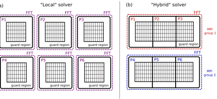
(a) "Local" solver (b) "Hybrid" solver

Figure 1: Parallelization strategies for pseudo-spectral Maxwell solvers. (a) is a sketch of the ’Local’ approach where the simulation domain is split into multiple sub-domains with guard cells appended at each sub-domain boundary. Guard cells hold copies of electromagnetic fields from adjacent sub-sub-domains. Each sub-domain is handled independently by an MPI process. At each time step: (i) Maxwell’s equations are advanced independently on each MPI sub-domain using shared-memory ’local’ FFTs and (ii) guard cells are exchanged between adjacent MPI sub-domains. Panel (b) shows a sketch of the new ’hybrid’ approach presented in this paper. It consists in grouping several MPI sub-domains into a larger MPI group and perform a distributed FFT on the MPI ranks of this group. Guard cells are solely appended at the boundary of the MPI group leading to less memory redundancy and thus significant memory savings. At each time step: (i) Maxwell’s equations are advanced independently on a MPI group using a distributed FFT. (ii) Guard cells are exchanged between MPI groups.

infinite order, imposes no Courant time step limit in vacuum and has no numerical dispersion. By lowering the resolution needed to reach a required accuracy compared to FDTD solvers [6, 7, 9], PSATD-type solvers have the potential to strongly re-duce the time-to-solution of a large class of problems.

1.2. Scalability limits of global FFT-solvers

Nevertheless, pseudo-spectral solvers employing distributed FFTs (later called ’global’ FTT solvers in the remainder of this article) have not been popular so far due to the difficulty to scale the distributed FFTs beyond 10,000 cores [10], which is not enough to take advantage of the largest supercomputers (with up to millions of cores) required for 3D modeling.

The main barrier to scale FFT computations emerges from the overhead induced by the global communications (’All’ to ’All’-type communication) required to transpose the data among all computing units. As a consequence, developing mas-sively parallel distributed FFTs algorithms is extremely chal-lenging and is still an active research area for computer scien-tists.

1.3. Recent advances in the scaling of FFT-based Maxwell solvers

To break this scalability barrier, a pioneering grid decom-position technique was recently proposed for pseudo-spectral FFT-based electromagnetic solvers [11]. This technique con-sists in using a standard Cartesian domain decomposition strat-egy to parallelize pseudo-spectral solvers (cf. Fig. 1- (a)). Maxwell’s equations are solved independently on each MPI processor sub-domain using local FFTs (instead of a single

global distributed FFT). Guard cells are exchanged between ad-jacent sub-domains at each time step. This technique is much more local and can be efficiently scaled providing that the num-ber of guard cells is not too high. It comes however with small stencil truncation errors at sub-domain boundaries when the stencil widthp/2 is higher than the number of guard cellsng. An important theoretical study [12] recently derived the analyt-ical expression for the amplitude and phase of these truncation errors. It showed that choosing a very high but finite order p stencil can already strongly reduce truncation errors compared to infinite order while still ensuring extreme accuracy. The model also pointed out that very high order solvers p > 100 can be used with a moderate number of guard cells (ng≪p/2) while still guaranteeing low levels of truncation errors (poten-tially below machine precision). By providing the number of guard cells required to obtain a given level of truncation error as a function of solver order, time step and mesh size, this model is crucial to enable the parallelization technique in production simulations.

This new type of based solvers (later called ’local’ FFT-based solvers) has been implemented and optimized in the high performance library PICSAR [5, 7]. They led to very good scal-ing on up to a million cores even for a moderate (ng < 10) number of guard cells and high solver orders p = 100. They notably enabled the very first accurate 3D simulations of laser-plasma mirror interactions [7, 13, 14] that were used to interpret the latest experimental results at CEA Saclay obtained with the 100TW UHI100 laser.

215 216 217 218 # cores 26 27 28 29 210 211 Ti m e /1 00 it (s) 215 ₂16 ₂17 ₂18 # cores 25 26 27 28 29 Ti m e /1 00 it (s) 215 ₂16 ₂17 ₂18 # cores 213 214 215 216 217 218 T o ta l m e m ( G B ) (a) (b) (c) n_g=8 n =16_g n =32_g

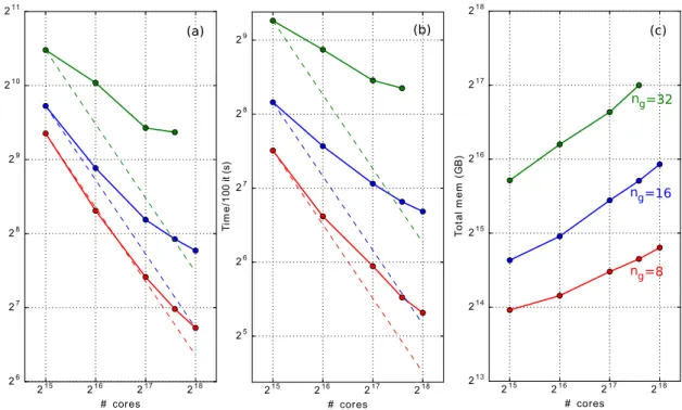
Figure 2: Evolution of strong scaling and memory consumption (grid quantities) of the pseudo-spectral PIC algorithm with the number of guard cellsngused (8

guard cells: red, 16 guard cells: blue, 32 guard cells: green) on Cray XC40 THETA cluster at ALCF (using 32768-262144 KNL cores) with one OpenMP thread per MPI. The FFTs are computed using the Intel MKL library. The simulation box consists in a homogeneous plasma with one particle per cell for both electrons and ions. Grid size: 240 x 6144 x 12288 grid cells. Panel (a) represents the scaling of the full PIC loop. Panel (b) represents the scaling of the pseudo-spectral solver only, including MPI-exchanges for grid quantities. Panel (c) represents the total memory consumption of grid quantities (ie field quantities).

1.4. Need for a more general massively parallel FFT-based Maxwell solver

Yet, local FFT-based solvers may not be adapted to the mod-eling of certain classes of problems where the level of trunca-tion errors need to be lower than machine precision for instance. In that case, the number of guard cells requiredng might be higher and can strongly affect the strong or weak scaling of the local solver.

This is illustrated on Fig. 2 where we compared the strong scaling of the local solver for different numbers of guard cells. As we can see on panels (a) and (b), although cases with a mod-erate number of guard cells succeed in keeping a good strong scaling, cases with a high number of guard cells quickly loose efficiency as the number of processors is increased. We can also note on panel (c) that due to an increased data redundancy, the total volume of memory required grows considerably as the number of guard cells/processors is increased.

Both limitations in terms of memory consumption and strong scaling of the local solver call for new parallelization strategies allowing for the use of an arbitrarily high number of guard cells. In this article, we present a novel massively parallel pseudo-spectral solver that ensures excellent strong/weak scaling at large scale (up to 800k cores) while allowing for the use of high number of guard cells to significantly reduce truncation errors. The remainder of the paper is divided into three additional sec-tions:

1. In section 2, we present the principle of the new paral-lelization method and its implementation in the high per-formance PIC library PICSAR,

2. In section 3, we present the benchmarks of the novel method on two large clusters (MIRA and THETA) available at the Argonne Leadership Computing Facility (ALCF),

3. In section 4, we conclude by presenting the perspectives brought by this novel method for the field of laser-plasma interaction.

2. Generalized massively parallel FFT-based Maxwell solver

In this section, we propose a new parallelization technique for the FFT-based Maxwell solver. This new type of FFT-based solver (later called ’hybrid’ FFT-based solver) is a more general approach than the local solver as it permits the use of an arbi-trary high number of guard cells while still ensuring extremely good scalability.

2.1. Principle of the new solver

The principle of the hybrid solver is illustrated on Fig. 1- (b). Adjacent MPI sub-domains are grouped into MPI groups (two groups on Fig. 1- (b)). Guard cells are now solely appended to the MPI group boundaries (and not to each MPI sub-domain boundaries). At each time step: (i) Maxwell’s equations are advanced independently on a MPI group using a distributed FFT and (ii) guard cells are exchanged between adjacent MPI groups.

As we now detail, this solver allows for significant memory savings as well as a reduction of the total volume of data exchanged.

2.2. Advantages in terms of memory

Let us assume a cubic mesh of sizenx×_ny×_nz=n3_splitted intonpMPI sub-domains along each directionx,yandz. Ifng guard cells are used for each MPI sub-domain, the total memory occupied by electromagnetic field arrays varies as:

Mloc_tot =O       n 3 p× " n np +2ng #3       (1)

As expected, one can notice that this memory strongly in-creases with the number of guard cellsng. In addition, the max-imum number of processors that can be used along each axis for this problem is given by _nn

p = ng, for which the total memory

used culminates to:

M_totloc=27Mn (2)

where Mn would be the total memory occupied by field arrays without any extra memory coming from guard cells. This maximum limit Mloc

tot does not depend on the number of guard cellsng. However, this maximum limit is attained for a much lower number of processors when ng ≫ _{1, potentially}

limiting the maximum number of processors that can be used due to memory limitations.

Let us now assume that MPI domains are grouped and that we usenmpiMPI processes per group along each axis. In this case, the total memory occupied by electromagnetic field arrays varies as: M_tothyb=O        n3 p n3 mpi × " _n npnmpi+2ng #3       (3) For_nn p =ng, we now obtain: Mhybtot = 2+nmpi nmpi !3 Mn (4)

The memory gain of the hybrid solver compared to local solver for the maximum limit of _nn

p =ngis thus: G3= M loc tot Mhyb_tot =3 3 nmpi 2+nmpi !3 (5) If we only make MPI groups alongd axes (d 63), this for-mula becomes:

Gd =3d nmpi

2+nmpi

!d

(6) The number of axisdalong which MPI sub-domains can be grouped directly depends on the number of axis along which the distributed FFT can be parallelized. For the FFTW library [15] (1D slab decomposition) we can parallelize the distributed

0 10 20 30 40 50 60 nmpi 0 10 1 20 2 30 G d

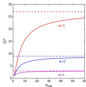
Figure 3: GainGd _{in terms of memory of the hybrid approach compared to}

the local approach (corresponding tonmpi =1). The curves representsGd as

a function of the number of MPI sub-domains per groupnmpi for d=1

(pur-ple curve), d=2 (blue curve) and d=3 (red curve). Dashed lines represent the

asymptotic limit ofGd_whenn

mpi>>1.

FFT alongzonly (in Fortran) and thus group MPI sub-domains solely alongz(i.ed = 1). For the P3DFFT library [16] (2D pencil decomposition), the distributed FFT can be parallelized alongyandzand MPI subdomains can therefore be grouped along two directions (i.e. d=2). The gainGd _{as a function of} nmpi is plotted on Fig. 3 for different values ofd =1,2,3. One can notice that for a fewnmpi >10 per groups, the total gain can already approach its maximum asymptotic value (G = 27 ford=3,G=9 ford=2 andG=3 ford=1).

2.3. Gains in terms of volumes of guard cells data exchanged Similarly, one can estimate the gain in terms of volume of guard cells data exchanged between the hybrid and local ap-proaches in the limit _nn_p =ng:

Gd_guard = M loc tot −Mn M_tothyb−_Mn = 3d₋₁ 1+2/nmpid−₁ (7)

For instance, the maximum gain on the total volume of guard cell exchanged ford =2 (with P3DFFT) andnmpi =5 can be as large as 8.

2.4. Advantages in terms of execution time of the FFT

Another important time gain expected from our hybrid par-allelization technique emerges from the execution time of the FFT. In the following, we first estimate the time complexity of the distributed FFT algorithm. In the light of this estimate, we then present the advantages of the hybrid solver compared to the local and global solvers.

2.4.1. Estimate of distributed FFTs computation time

Assessing the complexity of distributed memory FFT is important to understand and take advantage of the scalabil-ity of the hybrid solver. Distributed-memory FFTs perfor-mance strongly depends on both communication network and computer architecture. For multi-dimensional FFTs, most distributed-memory FFT libraries follow the same computation scheme detailed below. For each axis A of a 3D array:

1. If processors have all data in their local memory alongA, directly compute FFT alongA.

2. If data alongAis distributed on different processors, first transpose the 3D array so that each processor have all data alongAand then compute FFT alongA.

Following this computation scheme, we define the total time to perform a 3D FFT as the sum of the time required to trans-pose dataTtrand the time to compute the FFTsTc:

TFFT =Tc+Ttr (8)

The time complexity of a 3D FFT is known to be:

Tc=αn3logn3 (9)

where n is the global array size along each axis and α a machine-dependent parameter.

For a distributed-memory FFT with pencil decomposition, the data is distributed overnproc =n2pprocessors. In this case assuming perfect scaling, the computation timeTcper proces-sor is: Tc=α n 3_logn3 nproc ! (10) On the other hand, the transpose time Ttr is very network depend. Following the same reasoning as in [16] to estimate the communication time of the transpose operation, we get:

Ttr=β n 3 σbi[nproc] ! +γ n 3 nproc.σmem ! (11) whereσbi(nproc) is the bisection bandwidth of the network, βandγtwo machine and network dependent parameters and σmemis the memory bandwidth per MPI task.

For a large number of MPI tasks, we can neglect the term γ_n n3

proc.σmem compared to β n3

σbi[nproc] in eq (11) as the inter-node data transposition is more costly than the intra-node data-transposition (which only requires memory copies).

The bisection bandwidth is a function of the number of pro-cessors and depends on the nature of the supercomputer inter-connection network. For a 5D torus network such as the one equipping the IBM BG-Q MIRA cluster at the ALCF,σbi[nproc] should scale as nproc4/5. For the case of the THETA cluster (equipped with a Dragon fly network),σbi[nproc] should scale asnproc. In practice, we estimated the bisection bandwidth by fitting the global transposition time as a power of nproc. For both MIRA and THETA, the best fit found forσbi[nproc] scales as nproc4/5. For THETA, this is lower than the expected the-oretical value ofnproc. As opposed to MIRA where compute

nodes are allocated contiguously, compute nodes on THETA can be allocated at remote locations on the network, depending on the cluster occupancy at a given time. This might explain the lower-than-expected bisection bandwidth on THETA. Based on the bisection bandwidth estimates, we therefore used the fol-lowing expression ofTFFTfor both machines:

TFFT =α n3_logn nproc +β n3 nproc4/5 (12) 22 ₂6 ₂10 ₂14

# of MPIs per group (Theta)

10 20 30 40

Time

pe

r 1

00

FF

T

Lo

ca

l so

lve

r

Glo

ba

l so

lve

r

# MPIs per group (MIRA)

5 15 25

Time

pe

r 1

00

FF

T

Glo

ba

l so

lve

r

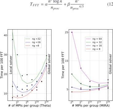
Figure 4: FFT total execution time as a function of the total number of MPI processes per group and the number of guard cells. The left panel represents the data from Theta and the right pane represents the data from Mira. Dots represent measured FFT execution time while dashed lines represent the fitting curve following eq 12

From formula (12), one can understand why distributed-memory FFTs do not scale well at large scale on massively par-allel computer architectures: for a large number of processors and a relatively small array size, the transpose operation will dominate the FFT computationαlog_n n

proc

≪ β

n4proc/5

hence resulting in a poor scaling proportional to 1/n4proc. On the other hand, for/5 large scale data set and relatively small number of processors, the computation term of the FFT will dominate the total time andαlog_n n

proc

≫ β

n4proc/5 thus resulting in a good scaling proportional to 1/nproc.

2.4.2. Advantages of the hybrid solver over local and global solvers

In the light of eq (12), one can note that our hybrid solver makes it possible to reduce the relative weight of the transpose operation timeTtrin the total FFT timeTFFT by properly tun-ing the number of MPI processes per groupnmpi on which the distributed FFT is performed. This should lead to a better per-formance than purely global solvers in most cases.

In addition, the hybrid solver should also outperform the lo-cal solver at large slo-cale. Indeed, one can show that the execu-tion time for the FFT (neglecting guard cell exchanges) for the local solver scales as:

T_FFTloc ∝n " n np +2ng #2 logn " n np +2ng #2 (13) where we assumed a 2D domain decomposition. For a large number of processorsnpsuch asn/np →_{ng, the execution time}

Tloc

FFT becomes constant and the parallel efficiency of the local solver drops considerably. In contrast, for the Hybrid solver this execution time should write:

T_FFThyb ∝ n n2_mpi " n np nmpi+2ng #2 log n n2_mpi " n np nmpi+2ng #2 (14) where we assumed a 2D pencil decomposition and a negligible transpose time compared to the FFT computation time. Choos-ing large enough MPI groups such thatn/npnmpi ≫_ngtherefore

leads to: T_FFThyb ∝ n 2 n2 p logn 2 n2 p (15) which would ensure very good scaling of the hybrid solver at large scale.

2.4.3. Benchmarks of the hybrid solver vs local and global solvers

To demonstrate the superiority of the hybrid solver over lo-cal and global solvers, many 3D simulations were run on both THETA and MIRA where the number of guard cellsngand MPI processes per groupsnmpi were varied (cf. Fig. 4). In all these simulations, we used the P3DFFT library (pencil decomposi-tion) to perform the distributed FFTs allowing to groupnmpi,y andnmpi,zMPI processes along theyandzdirections. Below are given details of the 3D cases run on MIRA and THETA:

• _{On MIRA: the array size per direction was chosen to}

n = 2048 and the number of guard cellsng = 8, 16 and 64. 8192 BG/Q nodes were used with 8 MPI processes per node (total of 216MPI tasks). For each case, the total num-ber of MPI processes per groupnmpi,y×nmpi,zwas varied as follows: 24, 27, 210, 213and 216, withnmpi,y×nmpi,z =216 corresponding to the global solver andnmpi,y×nmpi,z = 1 to the local solver.

• On THETA: the array size was chosen to 512×₄₀₉₆×

4096 cells and the number of guard cellsng =8,ng=16, ng = 32. 512 KNL nodes were used with 64 MPI per node for a total of 32768 MPI tasks. Two MPI tasks were used along the xdirection. The rest of the 16384 MPI tasks were split equally along y and z. The number of MPI processes per group along y and z direction was varied fromnmpi,y×nmpi,z=214(global solver), tonmpi,y×nmpi,z= 1 (local solver).

For each simulation, we collected the averaged execution time of FFTs among all MPI ranks. We chose to use the av-eraged time between these ranks since the problem was very well load-balanced between MPI processes (standard deviation of execution time did not exceed 10% among all MPI ranks). These execution times are displayed using colored markers on

Fig. 4. From these execution times, we could estimate the val-ues of the parametersαandβin the theoretical expression of TFFT (cf. eq (12)) using a least square algorithm. On MIRA, we obtainedα=1.andβ=1.5414. On THETA, we obtained α=1.andβ=67.1 We checked that using different box sizes and other simulation parameters led to similar results on both Theta and MIRA. One can see on Fig. 4 (cf. dashed lines) that the least square fit obtained leads to an acceptable matching be-tween expected and measured timings.

Fig. 4 shows the optimal number of MPI processes per group that minimizes the total execution time increases with the num-ber of guard cells. For a low numnum-ber of guard cellsng = 8, a few MPI processes per group (around 8) seems the best ap-proach whereas for a higher number of guard cellsng = 16, 20 MPI processes per group are required. As a consequence, having a good guess about the values ofαandβon a given net-work/computer architecture can help tune the hybrid solver to take advantage of the performance boost of our hybrid solver. The procedure to find the optimal number of groups for given domain decomposition/cluster architecture will be automated and added to the PICSAR library.

Although the model of eq. (12) is quite simple and omits var-ious operations involved in the FFT computation (data transfer among one compute node/data transposition among one MPI task ...), the error between the fit and the measured timing does not exceed 22%. This can also be explained by the the fluctu-ation coming from the 1D FFT computfluctu-ation since thenlogn scaling is not perfect.

Further tuning can be done on different machines to predict the optimal number of MPI processes per group. This optimum lies between 1 (global solver) andnproc (local solver), depend-ing on the machine and the problem size. We have noted that MIRA can support rather large MPI groups while keeping a good scaling, whereas on THETA, our method gives better re-sults with smaller groups. For critical cases where _nn

p = ng

wherengis the number of guard cells, we have noticed that it is always better to use the hybrid solver since it gives a substantial gain in terms of performance and memory saving.

2.5. Coupling of the hybrid Maxwell solver with the PIC algo-rithm

2.5.1. Brief reminder of the PIC algorithm

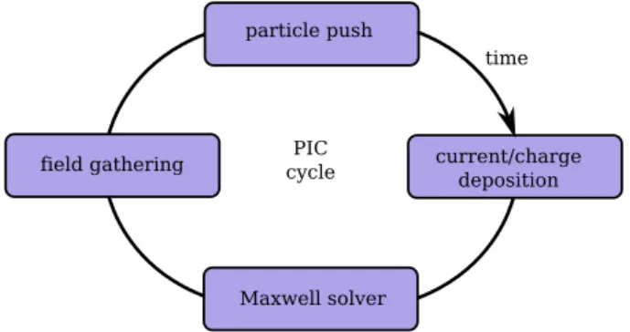
particle push current/charge deposition Maxwell solver field gathering time PIC cycle

The PIC algorithm self-consistently resolves Maxwell’s equations on a grid and motion equations of plasma pseudo-particles . The successive steps of the PIC cycle are sketched on Fig. 5. At each time step:

• _{particles are advanced using equations of motion (particle}

push) knowing the values of the electromagnetic fields at their position,

• _{once particles are advanced, current}/charge contribution of each particle on the grid is deposited using linear or higher order interpolation,

• _{once electromagnetic sources are known on the grid,}

Maxwell’s equations are solved to advance electromag-netic fields in time and space (Maxwell solver),

• _{once electromagnetic fields are known at next time step,}

field values are gathered from the mesh to particle’s posi-tion using interpolaposi-tion, usually at the same order as the deposition.

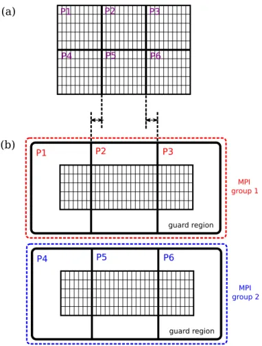
2.5.2. Dual grid decomposition for efficient load balancing All the difficulty in coupling the hybrid solver with the PIC algorithm lies in the efficient load balancing of (i) the particle and particle-mesh operations (particle push, field gathering, current/charge deposition) on the one hand and (ii) the Maxwell solver on the other hand. This has been illustrated on panels (a) and (b) of Fig. 6.

Panel (a) shows the domain decomposition D1 used to ef-ficiently load balance particle and particle/mesh operations (plasma is assumed to be homogeneous). Limits of MPI sub-domains are highlighted using black solid lines. Guard cells re-quired for particle-mesh operations (deposition/gathering) and of width equal to the order of deposition/gathering have not been represented for more clarity.

Panel (b) shows the domain decompositionD2that would be required to efficiently load balance the FFTs in the Maxwell solver step. One can see that in that case, the limits of MPI sub-domains inD1do not coincide with the limits of MPI sub-domains inD2 due to the presence of guard cells appended at the MPI group boundaries and needed in the computation of FFTs.

Load balancing all steps of the PIC loop thus requires keep-ing two different grids: (i) one grid G1 for the particle and particle-mesh operations (ii) one gridG2 for the FFTs. Note that the additional gridG1is also usually employed for smooth-ing [17] or mesh refinement [18] in the PIC algorithm. This comes with a slight additional memory cost (≈ _{30%) that yet}

still allows for large total memory gain thanks to the decrease of guard cells data redundancy with the hybrid solver.

We now detail how the coupling between the two grids is managed in the PIC cycle. At each time step:

1. Fields fromG1are copied toG2(including copies of data to the guard cells of MPI groups inG2). Overlapping grid regions pertaining to same MPI domains onG1andG2are

P1 P2 P3 guard region MPI group 1 P4 P5 P6 guard region MPI group 2 P1 P2 P3 P4 P5 P6 (a) (b)

Figure 6: Dual domain decompositions used to load balance (a)

particle-mesh/particle operations of the PIC loop (b) FFT computations of the Maxwell

solver step.

simply copied fromG1 toG2. Other regions ofG2 are updated using MPI exchanges of grid data fromG1toG2, 2. Maxwell’s equations are solved using the hybrid solver on

G2,

3. After the Maxwell solve step, field data (without guard cells) are copied fromG2toG1. Overlapping grid regions pertaining to same MPI domains onG2andG1are simply copied fromG2 toG1. Other regions ofG1 are updated using MPI exchanges of grid data fromG2toG1.

Note that this implementation does not actually require direct exchanges of guard cell data between MPI groups as mentioned in the previous section. Guard cells ofG2 are instead directly filled fromG1during the first step of the coupling.

2.6. Implementation in the PICSAR library

The Particle-In-Cell Scalable Application Resource (PIC-SAR) [19, 5] is an open-source high performance library in-tended to help scientists porting their code to the next genera-tion of exascale computers. PICSAR contains highly optimized PIC routines exploiting the three levels of parallelism that mod-ern architectures offer (Internode parallelism, Intranode paral-lelism, Vectorization) as well as optimized parallel I/O routines. The hybrid Maxwell solver has been fully implemented in PICSAR and can currently be used by the WARP [20, 21] and

215 ₂16 ₂17 ₂18 20 21 Mem ory G ain

ng = 8

Figure 7: Local vs Hybrid+slab decomposition on THETA. Each panel represents a different number of guard cells.The blue curves stand for the hybrid solver

data, while the red curves stand for the local solver data. The green line represents the total memory gain brought by the hybrid solver compared to the local solver.

WARPX [18] codes. Note that the WARPX code also imple-ments a slightly different version of the dual domain decompo-sition presented in this paper, which won’t be presented here.

PICSAR is written in Fortran 90 and can be compiled in three different modes:

• _{As a Python module that can be directly coupled with other}

codes also using python as the outermost software layer. Right now, PICSAR is coupled to the WARP PIC code through this layer,

• _{As a static/dynamic library to be used by other}

For-tran/C/C++codes. For instance, the WARPX and SMILEI [22] PIC codes are presently coupled to PICSAR by this means,

• _{As a self-consistent Fortran 90 PIC code. All tests}

per-formed in this paper have been done through this mode. To perform the distributed FFTs, PICSAR can use either the FFTW or P3DFFT libraries:

• _{FFTW is a well-established GPL FFT library that can}

per-form shared-memory/distributed FFTs . The distributed FFT only supports parallelization along one axis (slab de-composition), which is the last axis or z-axis in Fortran.

• _{P3DFFT is an open source library that can perform}

dis-tributed FFTs using a pencil domain decomposition. By offering parallelization over two axis, P3DFFT there-fore offers more flexibility than the distributed version of FFTW. To compute the FFTs locally, P3DFFT makes use of existing shared-memory versions of other FFT libraries (currently it only supports FFTW, ESSL).

Note that on Intel architectures, such as THETA, the MKL library can be used instead of FFTW through the FFTW-MKL wrapper, which allows performing DFT computations with the MKL library without modifying FFTW directions. All per-formance tests performed on THETA whether using FFTW or P3DFFT have been done with MKL-FFTW support for shared-memory FFTs, as this proved to bring better performance for both local and hybrid solver. On MIRA, P3DFFT (with FFTW support for shared-memory FFTs) and FFTW were used. To use the hybrid solver, the user needs to specify some additional simulation parameters related to the hybrid solver. These pa-rameters are :

• _{the FFT library used for distributed FFTs (FFTW or}

P3DFFT),

• _{the number of groups along y and z direction (in the}

z-direction only when using FFTW),

• _{the number of group guard cells along y and z direction (in}

the -direction only when using FFTW),

• _{an additional flag to enable/disable the use of ”optimized}

communication strategy” to compute FFTs (Only available in 3D). The ”optimized communication strategy” skips the last data transposition after each FFT in order to save com-putational time. Indeed the last transposition is only re-quired to have the same data layout for the output array and the input array. This saves computational time but results in a different layout of field arrays in the Fourier space that needs to be taken into account when solving Maxwell’s equations. This has been included in PICSAR that benefits from this optimization for both P3DFFT and FFTW modes in 3D simulations.

215 ₂16 ₂17 ₂18 21 22 23 Mem ory G ain

ng = 8

Figure 8: Local vs Hybrid+pencil decomposition on THETA. Each panel represents a different number of guard cells. The blue curves stand for the hybrid solver

data, while the red curves stand for the local solver data. The green line represents the total memory gain brought by the hybrid solver compared to the local solver.

Besides, note that when using the hybrid solver, PICSAR cal-culates the MPI groups topology and createsngroupMPI sub-communicators, each sub-communicator being appended to a unique group. The data sizes on each MPI task is set by the FFT library, which results in a new domain decomposition re-lated to the Maxwell’s equations solve as illustrated on Fig. 6 (b). Finally, FFT plans are initialized by the FFT library on each group.

The intersection between the two domain decompositions is computed before the PIC loop starts, and a data exchange protocol is determined according to the grid overlaps. If dy-namic load-balancing is enabled for the simulation, then this pre-processing step needs to be recomputed accordingly. In practice, the data exchange step is rather computationally cheap and does not add an important overhead to the PIC loop since the majority of data exchanges are simple data copies within the same MPI process. In PICSAR, the data exchange protocol is done in a way that allows both blocking and non-blocking MPI exchanges.

Finally, note that the PICSAR FFT-based Maxwell solver now also supports absorbing boundary conditions implemented using the two-step Perfectly Matched Layers algorithm recently developed in [23].

3. Benchmark of the new solver at very large scale

The new solver has been benchmarked on both THETA and MIRA at very large scale. All benchmarks considered the sim-ulation of a 3D homogeneous plasma with 1 pseudo-particle per cell for both electrons and ions. These benchmarks are pre-sented below.

3.1. Benchmark on THETA

The hybrid solver on THETA has been benchmarked us-ing both P3DFFT and FFTW MPI libraries. On THETA, the FFTW-MKL wrapper has been used with FFTW MPI and P3DFFT.

3.1.1. Benchmark with the slab decomposition

The box size is nx × ny × nz = 160 × 160 × 393216 cells, where larger array sizes were used along z to investi-gate strong scaling for a large number of processors. Mul-tiple simulations were run with different numbers of guard cells ng = 8,16,32. The number of KNL nodes used was Nnodes = 512,1024,2048,3072,4096 with 64 MPI tasks per node and one OpenMP thread per MPI task. For each simu-lation we usednmpi =32 MPI processes per group.

As shown on Fig. 7, the slab decomposition allows a mem-ory and performance gain of order×_{2.5 against the local solver,}

for a high number of guard cells. The strong scaling efficiency of the hybrid solver for 32 guard cells is 87% between 512 and 3072 KNL nodes, while the local solver efficiency is only about 47%. Besides, note that the hybrid solver allows to run simu-lations on more nodes than the local solver which is limited by

n

np =ng(note that the last point of the 32 guard cells simulations with the local solver is missing.

3.1.2. Benchmark with the pencil decomposition

In this benchmark the grid size wasnx×ny×nz=240×6144× 12288, where a larger size was chosen alongycompared to the slab decomposition. We kept the same number of guard cells as for the slab benchmark (ng=8,16,32). The number of MPI processes per group was fixed to 64. We used 64 MPI processes per node and one OpenMP thread/MPI task for all the tests.

213 ₂14 ₂15 ₂16 ₂17 ₂18 ₂19

2

2

2

Figure 9: Local vs Hybrid+pencil decomposition on MIRA. Each panel represents a different number of guard cells. The blue curves stand for the hybrid solver

data, while the red curves stand for the local solver data. The green line represents the total memory gain brought by the hybrid solver compared to the local solver.

Results of this benchmark are displayed on Fig. 8. Here again, the hybrid solver performs much more efficiently than the local solver at large scale (especially for a large number of guard cells) both in terms of time-to-solution (up to×₄

speed-up) and memory used (up to×_{8 less memory).}

3.2. Benchmark on MIRA

On MIRA,the hybrid solver was benchmarked using the pen-cil decomposition only. The grid size was nx ×ny ×nz =

256×₂₀₄₈×_{2048 cells. All the simulations were ran with 4}

OpenMP threads per MPI process. Each MPI group was com-posed of 256 MPI tasks. The number of nodes was varied be-tween 512 to 16384.

This benchmark (cf. Fig 9) shows again a very good strong scaling of the hybrid solver and a very good parallel efficiency at large scale. Moreover, we show that MPI exchanges involved in the PIC loop (apart from the global exchanges involved in the FFT transpose) are less costly when using the hybrid solver (due to a decrease of the total volume of MPI exchanges).

4. Conclusion

We presented a novel massively parallel technique for ultra-high order FFT-based Maxwell solvers. As opposed to the previously developed ’local’ technique, this ’hybrid’ technique (which performs distributed FFTs on groups of neighbouring MPI processes) is very general and allows a very good strong scaling for an arbitrarily high number of guard cells. For large numbers of guard cells, it notably increases the maximum num-ber of MPI processes that can be used to parallelize computa-tions. Besides, by reducing data redundancy, it also has huge benefits in terms of memory savings compared to the ’local’

technique for a given problem size. Both the improvements in strong scaling and memory savings will enable larger 3D PIC simulations than previously accessible with the ’local’ tech-nique.

Acknowledgements

The authors would like to thank R´emi Lehe and Julien Der-ouillat for fruitfull discussions.

This research was supported by the Exascale Computing Project (ECP), Project Number: 17-SC-20-SC, a collaborative effort of two DOE organizations the Office of Science and the National Nuclear Security Administration responsible for the planning and preparation of a capable exascale ecosystem in-cluding software, applications, hardware, advanced system en-gineering, and early testbed platforms to support the nations exascale computing imperative.

This work was supported in part by the Director, Office of Science, Office of High Energy Physics, U.S. Dept. of Energy under Contract No. DE-AC02-05CH11231.

An award of computer time (PICSSAR INCITE) was pro-vided by the Innovative and Novel Computational Impact on Theory and Experiment (INCITE) program. This research used resources of the Argonne Leadership Computing Facility, which is a DOE Office of Science User Facility supported under Contract DE-AC02-06CH11357.

References

[1] R W Hockney and J W Eastwood. 1988.

[2] C K Birdsall and A B Langdon. Adam-Hilger, 1991.

[4] Ricardo A Fonseca, Jorge Vieira, Frederico Fi´uza, Asher Davidson, Frank S Tsung, Warren B Mori, and Luıs O Silva. Exploiting multi-scale parallelism for large scale numerical modelling of laser wakefield

accel-erators.Plasma Physics and Controlled Fusion, 55(12):124011, 2013.

[5] Henri Vincenti, Mathieu Lobet, Remi Lehe, Jean-Luc Vay, and Jack

Deslippe. 17 pic codes on the road to exascale architectures.Exascale

Sci-entific Applications: Scalability and Performance Portability, page 375,

2017.

[6] G Blaclard, H Vincenti, R Lehe, and JL Vay. Pseudospectral maxwell solvers for an accurate modeling of doppler harmonic generation

on plasma mirrors with particle-in-cell codes. Physical Review E,

96(3):033305, 2017.

[7] Henri Vincenti and Jean-Luc Vay. Ultrahigh-order maxwell solver with

extreme scalability for electromagnetic pic simulations of plasmas.

Com-puter Physics Communications, 228:22–29, 2018.

[8] I Haber, et al.,.Proc. Sixth Conf. Num. Sim. Plasmas, pages 46–48, 1973.

[9] S ¨oren Jalas, Irene Dornmair, R´emi Lehe, Henri Vincenti, J-L Vay, Manuel Kirchen, and Andreas R Maier. Accurate modeling of plasma acceleration

with arbitrary order pseudo-spectral particle-in-cell methods. Physics of

Plasmas, 24(3):033115, 2017.

[10] S. Habib, et al.,.arXiv.org, page 1211.4864.

[11] J.-L. Vay, I. Haber, and B. B. Godfrey. J. Comput. Phys., 243:260–268,

2013.

[12] H. Vincenti and J.-L. Vay.Comput. Phys. Comm., 200:147–167, 2016.

[13] H Vincenti. Achieving extreme light intensities using relativistic plasma

mirrors.arXiv preprint arXiv:1812.05357, 2018.

[14] L Chopineau, A Leblanc, G Blaclard, A Denoeud, M Th´evenet, JL Vay,

G Bonnaud, Ph Martin, H Vincenti, and F Qu´er´e. Identification of cou-pling mechanisms between ultraintense laser light and dense plasmas.

arXiv preprint arXiv:1809.03903, 2018.

[15] http://www.fftw.org/.

[16] Dmitry Pekurovsky. P3dfft: A framework for parallel computations of

fourier transforms in three dimensions.SIAM Journal on Scientific

Com-puting, 34(4):C192–C209, 2012.

[17] Brendan B. Godfrey and Jean-Luc Vay. Suppressing the numerical

cherenkov instability in fdtd pic codes.Journal of Computational Physics,

267:1 – 6, 2014.

[18] J-L Vay, A Almgren, J Bell, L Ge, DP Grote, M Hogan, O Kononenko, R Lehe, A Myers, C Ng, et al. Warp-x: A new exascale computing

plat-form for beam–plasma simulations.Nuclear Instruments and Methods in

Physics Research Section A: Accelerators, Spectrometers, Detectors and

Associated Equipment, 2018.

[19] H. Vincenti, M. Lobet, R. Lehe, R. Sasanka, and J.-L. Vay.Comput. Phys.

Comm., 210:145–154, 2017.

[20] J.-L. Vay, D P Grote, R H Cohen, and A Friedman. Computational

Sci-ence and Discovery, 5(1):014019 (20 pp.), 2012.

[21] http://blast.lbl.gov/blast-codes-warp.

[22] Julien Derouillat, Arnaud Beck, F P´erez, T Vinci, M Chiaramello, A Grassi, M Fl´e, G Bouchard, I Plotnikov, N Aunai, et al. Smilei: a collaborative, open-source, multi-purpose particle-in-cell code for plasma

simulation.Computer Physics Communications, 222:351–373, 2018.

[23] Olga Shapoval, Jean-Luc Vay, and Henri Vincenti. Two-step perfectly matched layer for arbitrary-order pseudo-spectral analytical time-domain