Variational Tetrahedral Meshing

Variational Tetrahedral Meshing

Abstract

In this paper, a novel Delaunay-based variational approach to isotropic tetrahedral meshing is presented. To achieve both robust-ness and efficiency, we minimize a simple mesh-dependent energy through global updates of both vertex positionsandconnectivity. As this energy is known to be theL1_{distance between an isotropic} quadratic function and its linear interpolation on the mesh, our min-imization procedure generates well-shaped tetrahedra. Mesh design is controlled through a gradation smoothness parameter and selec-tion of the desired number of vertices. We provide the foundaselec-tions of our approach by explaining both the underlying variational prin-ciple and its geometric interpretation. We demonstrate the quality of the resulting meshes through a series of examples.

Keywords: Isotropic meshing,Delaunay mesh,sizing field,slivers.

1 Introduction

Three-dimensional simplicial mesh generation aims at tiling a bounded 3D domain with tetrahedra so that any two of them are either disjoint or sharing a lower dimensional face. Such a dis-cretization of space is required for most physically-based simula-tion techniques: realistic simulasimula-tion of deformable objects in com-puter graphics, as well as more general numerical solvers for par-tial differenpar-tial equations in computational science, need a discrete domain to apply finite-element or finite-volume methods. Most ap-plications have specific requirements on the size and shape of sim-plices in the mesh. Isotropic meshingis desirable in the common case where nearly-regular tetrahedra (nearly-equal edge lengths) are preferred.

Creating high quality tetrahedral meshes is a difficult task for a vari-ety of reasons. First, the mere size of the resulting meshes requires robust, disciplined data structures and algorithms. There are also basic mathematical difficulties which make tetrahedral meshing significantly harder than its 2D counterpart: the most isotropic 3D simplex, the regular tetrahedron, doesnottile 3D space (let alone specific domains), while the equilateral triangle does tile the plane; unlike the 2D case, even well-spaced vertices can create degenerate 3D elements such as slivers (see Fig.2). Dealing with boundaries is also fundamentally more difficult in 3D: while it always exists a 2D triangulation conforming to any set of non intersecting constraints, this is no longer true in 3D [Shewchuk 1998a]. All these facts ren-der both the development of algorithms and suitable error analysis for the optimal 3D meshing problem very challenging. Given that one can often observe in applications that the worst element in the domain dictates accuracy and/or efficiency [Shewchuk 2002a], it is clear that great care is required to design the underlying meshes and ensure that they meet the desired quality standards.

1.1 Previous Work & Nomenclature

The meshing community has extensively studied a number of tech-niques over the last 20 years. We do not aim at covering all

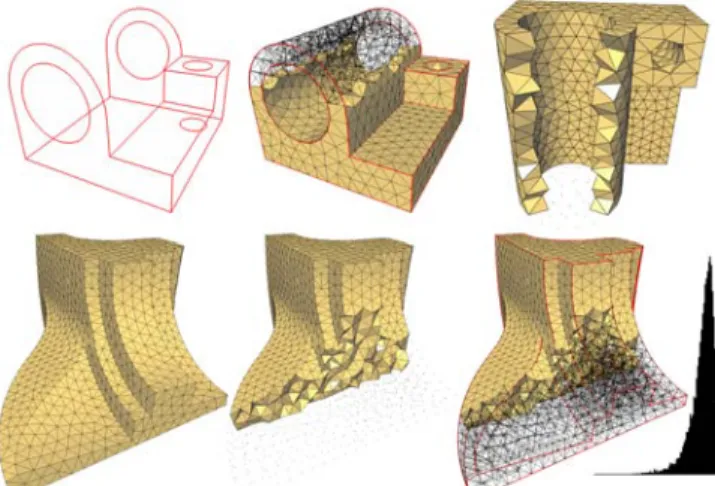
previ-Figure 1:Variational Tetrahedral Meshing: Given the boundary of a do-main (here, a human torso), we automatically compute the local feature size of this boundary as well as an interior sizing field (left, cross-section), be-fore constructing a mesh with a prescribed number of vertices (here65K₎ and a smooth gradation conforming to the sizing field (right, cutaway view). The resulting tetrahedra are all well-shaped (i.e., nearly regular). ous work since comprehensive surveys are available [Carey 1997;

Owen 1998; Frey and George 2000; Teng et al. 2000; Eppstein 2001]. To motivate our work we briefly review both the usual nomenclature and the main difficulties involved in isotropic tetra-hedral mesh generation. Throughouttetwill be the abbreviation for tetrahedron.

Proper mesh generation requires a number of successive stages, which are governed by a number of key factors:

Shape Quality Measures: Element shape/size requirements are typically application-dependent. Consequently, an extraordinar-ily large number of quality measures has been proposed, ranging from minimum or maximum bounds on dihedral or solid angles, to more complex geometric ratios. We recommend [Shewchuk 2002a] for a clear exposition of both the history behind these mea-sures and their relation to (1) the conditioning of finite element stiffness matrices and (2) the accuracy of linear interpolation of functions and their gradients. Among the most popular quality measures of a tet are the radius and radius-edge ratios. The lat-ter measures the ratio between the circumsphere radius and the shortest edge length. It is not afair measure since it does not approach zero for a class of degenerate tets calledslivers (sliv-ers result when four tet vertices are close to a great circle of a sphere and spaced roughly equally along this circle, see Fig.2). The radius ratio, which takes the quotient of inscribed and cir-cumscribed sphere radii (times three for normalization purposes),

isa good measure for any kind of degeneracy.

Figure 2:Tet shapes: the regular tet (leftmost) is well shaped, unlike the other tets displayed: each represents a type of degeneracy. The rightmost one with 4 near-cocircular vertices is usually referred to as asliver. Sizing requirement: Accuracy and efficiency of numerical

solvers depend on the local size of tets. Consequently, asizing field, prescribing the ideal local edge length as a function of space,

must be added. Obvious choices include the constant field for a uniform mesh, and a priori or a posteriori error estimators for sim-ulations. To avoid bad dihedral angles in the simplices one typi-cally requires the sizing field to vary smoothly [Ruppert 1993].

Boundary Requirements: Some approaches aim atconforming

to (i.e., matching exactly) the domain boundary by adding Steiner points if necessary [Cohen-Steiner et al. 2002;Krysl and Ortiz 2001;Cheng and Poon 2003]. Others require of the mesh bound-ary to onlyapproximatethe domain boundary. The latter allows for higher tet quality since the boundary is not required to match the input surface. In particular the latter is important when the initial input is a low quality surface triangulation.

Strategy: Existing meshing techniques can be roughly classified by the general strategy they employ:

Advancing front: Starting from the boundary of the domain, new vertices are added by a local heuristic to ensure that the generated tets have acceptable shapes and sizes and conform to the desired sizing field. Global optimization steps can also be performed sporadically to improve the mesh quality further. A number of variants exist, such as sphere or bubble packing [Li et al. 2000], which provide better tet shape and size control al-beit adding a significant computational overhead.

Octree-based methods: An octree is first refined until each of its leaves is either strictly inside or strictly outside of a finely voxelized version of the domain. Proper connections of the in-terior leaves through, for instance, a red-green strategy [Molino et al. 2003] then ensure a good initial mesh of the domain, usu-ally improved through optimization or physicusu-ally-based relax-ation in particular to better approximate the domain boundary. Other similar methods offer bounds of worst dihedral angles even without a relaxation stage [Mitchell and Vavasis 2000]. Unfortunately, octree-based meshes have preferred edge direc-tions, which may be detrimental to subsequent use in simulation.

Delaunay approaches: For a given set of sample points in

3D, itsDelaunay triangulationhas the canonical property of minimizing the maximum radius of the minimum containment sphere. This property is very useful in approximation theory: this radius provides an upper bound on theL∞difference be-tween any functionfand itspiecewise linear approximant, as-sumingf has bounded second derivatives. Thus a Delaunay triangulation provides good control over the worst interpola-tion error inside a domain. Consequently a large body of work in numerical analysis provides error estimates for a variety of applications using these meshes. Because of these as well as many other optimality properties, mesh generation relying on Delaunay triangulation such as Delaunay refinement [Ruppert 1993;Shewchuk 1998b;Shewchuk 2002b;Cheng et al. 2004], unit mesh [Borouchaki et al. 1997a;Borouchaki et al. 1997b], or centroidal Voronoi tessellations [Du and Wang 2003] have flourished in the meshing and Computational Geometry com-munities. Delaunay refinement methods offer some theoretical guarantees on the resulting meshes: they provide bounds on the radius-edge ratio, and are shown to be asymptotically optimal with respect to the number of elements in the mesh. Delau-nay refinement, however, can generate slivers; some attempts have been made to handle the sliver problem within Delaunay refinement [Cheng et al. 1999; Cheng and Dey 2002;Li and Teng 2001]. Unfortunately the theoretical guarantees are quite poor, and the mesh either is no longer Delaunaybut a regu-lar (weighted Delaunay) triangulation, or comes with degraded bounds on the radius-edge ratio.

Mesh Optimization Techniques: Even if fast and robust Delau-nay triangulators are available, the previous strategies can re-quire substantial implementation effort to make them robust to arbitrary input domains. A large number of practical meshing techniques instead employ local optimization methods which

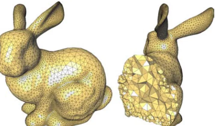
Figure 3:Stanford bunny: meshing the interior of the bunny with adapted tets (smaller near the boundary, larger inside, and smooth gradation (K= 1_{) in between). The cutaway views show the well-shapedness of the mesh} elements inside the domain; notice also the quality of the boundary mesh.

move vertices adjacent to poorly-shaped tets to improve mesh quality. Coupled with local face swapping between adjacent tets as well as tet insertions and deletions, these strategies can result in nice final meshes [Freitag and Ollivier-Gooch 1996;Cutler et al. 2004]. Unfortunately, these optimizations often use highly non-convex functionals and get easily stuck in local minima. From this brief overview we see that meshing has been approached with two very different emphases: theory and practice. Theoreti-cal methods, most commonly using iterative Delaunay refinement approaches, come with quality guarantees that are often not suited to further use in practical applications: the presence of fairly de-generated tets are a serious problem for many numerical methods. Alternatively, optimization methods provide viable solutions with relatively little implementation effort, and the quality obtained is satisfactory for a class of applications. Alas, their ad-hoc nature does not warrant high-quality meshes. When seeking high qual-ity meshes, a method combining optimization with solid theoreti-cal foundations would provide the best of both worlds, promising meshes of a quality that none of the existing approaches could ob-tain by themselves.

1.2 Approach and Contributions

In this paper, we present a Delaunay-based optimization technique, that we callVariational Tetrahedral Meshing, to efficiently mesh a bounded 3D domainΩof arbitrary topology or number of con-nected components. The domain boundary∂Ωis assumed to be a manifold, watertight and intersection-free triangular mesh. Draw-ing on recent work on surface approximation [Cohen-Steiner et al. 2004] and Optimal Delaunay Triangulations [Chen and Xu 2004], we propose a simple minimization procedure that alternates global 3D Delaunay triangulation and local vertex relocation to consis-tently and efficiently minimize a global energyover the domain. It results in a robust meshing technique that generates high qual-ity isotropic meshes in terms of radius ratios, as well as angles. A notable feature of the method is that it removes slivers inside the domain. To provide a flexible meshing tool, we also introduce an automatic sizing field construction that guarantees an arbitrary smooth gradation of the mesh together with faithful approximation of the domain boundary. Equipped with these tools, the user has full control over the mesh design, and can require a specific number of vertices for the final mesh. We demonstrate the versatility and ro-bustness of our method through a series of results and comparisons; we also give details on the current limitations.

2 Variational Approach to Meshing

Variational approaches (that is, methods relying on energy mini-mization) have been advocated as a powerful and robust tool in

meshing both in graphics for triangle [Hoppe et al. 1993; Cohen-Steiner et al. 2004] and tet [Molino et al. 2003;Cutler et al. 2004] meshes and in mechanical engineering for volumetric meshes [ Fre-itag and Ollivier-Gooch 1996;Du and Wang 2003]. These methods basically define (often highly) non-convex energies that they mini-mize through vertex displacements and/or connectivity changes in the current mesh. Our method also falls into this broad category. However, in contrast to earlier work, we use a simple quadratic energy (which we analyze) and allow for global changes in mesh connectivity during energy minimization. We will point out both the theoretical and practical consequences of such a strategy. We begin by motivating our choice of energy.

2.1 Consistent Energy Minimization

A few of these variational methods [Cohen-Steiner et al. 2004;Du and Wang 2003] have an attractive theoretical property resulting in remarkable results: vertex positionsand connectivity updates are performed alternately tominimize the same quadratic energy. This specificity has rich consequences. First, each update can be doneoptimallydue to the simplicity of the energy used. Second, assuming convexity of the boundary, the energy decreases mono-tonically, implying eventual convergence. Lastly, since both opti-mization steps minimize the same energy, their final meshes have a concrete, variational nature: the resulting meshes are (quasi) mini-mizers of a “quality” functional.

Centroidal Voronoi Tessellations Du and Wang [2003] pro-pose to generate meshes that aredualto optimal Voronoi diagrams. These diagrams are achieved by minimizing the quadratic energy:

ECVT= X i=1..N Z Vi ||x−xi||2dx (1) where thexiare vertex positions andVia local cell associated with

eachxi; the union of these cells forms a partition of the domainΩ.

Du and Wang used Lloyd relaxation [Lloyd 1957] to robustly mini-mize this energy: for a given set of vertices, compute their Voronoi diagram (restricted to the domainΩ) since itisthe energetically op-timal partition for the current vertex positions. In a second phase, the partition is held fixed and vertex positionsxi are optimized.

Even though these steps ofpartitioningand vertex position opti-mization are quite different in character, each of them decreases the same energy. Du and Wang explain how a mesh that minimizes this energy has each vertexat the centroidof its own Voronoi cell: hence the nameCentroidal Voronoi Tessellation(CVT). Aside from the theoretical properties of CVTs, Du and Wang also note the superior results they get in comparison to conventional Laplacian smooth-ing (a widespread technique in graphics due to its simplicity, but for which the associated energy only relies on edge length, not on spatial distribution).

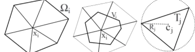
Figure 4: Nomenclature: Left: We denote byΩ_ithe 1-ring of vertexx_i. Middle:V_{iis the Voronoi cell of vertex}x_i. Right: The center of the circum-circle of triangleT_{j, is denoted}c_j, while its radius is denotedR_j. ¿From the analysis of ECVT it is well known that its

minimiza-tion corresponds to minimizing the volume between a paraboloid

f(x) = ||x||2and anunderlaid, circumscribing piecewise linear

approximantfdual

PWL, which is formed by planar patches tangent to the

paraboloid (see Fig.5(a)):

ECVT=||f−f dual PWL||L1.

In 2D, this approach will lead to isotropically sampled meshes since it has been shown that anyLp

optimal approximation of a

smooth function asymptotically tends to align and shape its ele-ments according to the eigenvectors and eigenvalues of its Hes-sian [Shewchuk 2002b]: since the Hessian of the quadratic function

f(x) =||x||2is isotropic, the resulting meshes must have nearly hexagonal Voronoi cells, i.e., nearly equilateral triangles in the dual Delaunay mesh.

Unfortunately, and despite Du’s proposal [2003] to use CVTs for tet meshing, there exists no proof of such a dual property in 3D. Our own tests show that using Du’s suggestion for tet meshing gives rise to numerous degenerateslivertets (see Fig.2). We can attribute the slivers to the fact thatECVTtends to optimizes the compactness of

the dual Voronoi cells, but not the compactness of simplices in the primal Delaunay triangulation: therefore, the presence of a sliver isnot penalized by this energy. In other words, this variational approach ensures that the vertices in the domain are well spaced (i.e., isotropic point sampling—see [Hardin and Saff 2004] for an overview of this interesting problem); sadly, having well-spaced vertices guarantees nothing in terms of the quality of the actual 3D mesh [Eppstein 2001].

Optimal Delaunay Triangulations Recently, Chen [2004] proposed an approach “dual” to the above in the context of mesh optimization. He used the following energy:

EODT=||f−f primal PWL ||L1,

i.e., the volume between a paraboloid and anoverlaid, circumscrib-ing piecewise linear approximantfprimal

PWL formed by a linear

interpo-lation of points on the paraboloid (see Fig.5(b)). Chen made the observation that changing the energy fromECVTtoEODTamounts to

only a slight change in Eq. (1), turning it into:

EODT= 1 n+ 1 X i=1..N Z Ωi ||x−xi||2dx. (2) The integral is now taken over each1-ringregionΩi(also called the

star of the vertexxi, see Fig.4). Notice that these regions overlap.

These quadratic energies differ quite significantly: Chen’sEODT

en-ergy measures a quality of thesimplicial mesh, not of its dual. It is thus more prone to generate well-shaped primal elements, while

ECVTwas maximizing the compactness of the dual Voronoi cells.

2 2

Figure 5:PWL approximations: A paraboloid can be approximated by an underlaid circumscribed PWL function (left), or by an overlaid one (right). Although no formal guarantee on the resulting meshes is given in [Chen and Xu 2004], the 2D results presented are of high qual-ity. The smoothing technique presented in [Chen 2004] updates the mesh connectivity through only-local edge flips when an inverted triangle is detected. Unfortunately, this local connectivity optimiza-tion in the 2D triangle case does not carry over to 3D: there is no theorem proving that an arbitrary mesh is only a few flips away from the optimal connectivity.

2.2 Our Variational Approach

We propose an algorithm to consistently minimize the primal en-ergyEODT. This is achieved not just through asmoothingprocedure

(as suggested in [Chen 2004]), but through a full-blown minimiza-tion procedure for both vertex posiminimiza-tionsandconnectivity.

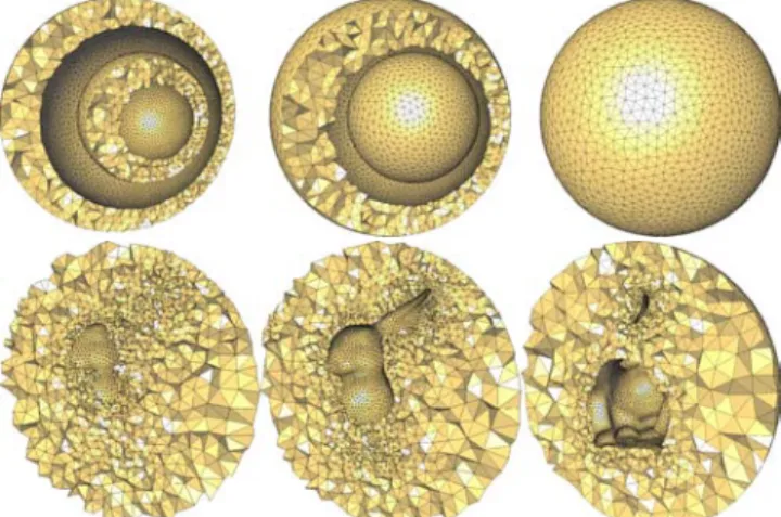
Figure 6:Complex Topology: As stressed in this paper, our approach can as well mesh complex domains with arbitrary genus. Four nested spheres define a multi-layer object (top); a bunny immersed in a sphere (bottom).

Optimizing Connectivity Connectivity optimization is easily achieved: for a given set of vertex positionsxi, its Delaunay

tri-angulation is again (remarkably!) theoptimal connectivity which minimizesEODT (as shown in [Chen and Xu 2004]) just as it is

optimal forECVT. Therefore, we compute the (global) Delaunay

connectivity systematically, guaranteeing optimality of the connec-tivity at each iteration.

Optimizing Vertex Positions One can show that for a given meshMwith verticesxi’s,EODTcan be written as:

EODT= 1 4 X i xi2|Ωi| − Z M x2dx, (3)

where|Ωi|is the measure (volume in 3D) of the 1-ring

neighbor-hood of vertexxi(AppendixBgives a short proof). Noting that the

last term is constant given a fixed boundary∂M, a simple deriva-tion of this quadratic energy inxileads to the followingoptimal positionx?i of the interior vertexxiin its 1-ring:

x?i =− 1 2|Ωi| X Tj∈Ωi     ∇xi|Tj| h X x k∈Tj x_k6=x_i ||xk||2 i     . (4)

The term∇xi|Tj|is the gradient of the volume of the tetTjwith

respect toxi. Replacing functionf(x) =||x||2 by the translated functionf(x) =||x−xi||2, which has the same interpolation error

and thus leads to the same optimal position, we get the following equivalent expression used to update a vertex position :

x?i=xi− 1 2|Ωi| X Tj∈Ωi  ∇xi|Tj| h X xk∈Tj ||xi−xk||2 i  . (5)

Geometric and Physical Interpretations As shown in the AppendixC, we can express the latter optimality condition in more obvious geometric terms, to further our understanding of the bene-fits of this variational approach:

x?i = 1 |Ωi| X Tj∈Ωi |Tj|cj. (6)

wherecjis the circumcenter of tetTj(see Fig.4). This last

expres-sion shows that, although we move each vertex to a local average, the optimal placement heavily depends on the local distribution. For instance, if all the 1-ring neighbors are on a common sphere, the optimal position will be the sphere center. In fact, as evidenced by Eq.4, this optimal location dependsonlyon the 1-ring neigh-bors, not on the current location. Note also the similarities with the

generalized barycentric coordinates in the Voronoi polytope pro-posed in [Warren et al. 2004].

If we further transform the energy (see AppendixB), we get:

EODT= X j |Tj|R2j− Z Tj ||x−cj||2dx= 2 X j |MSj−MTj| (7)

whereMTj is the sum of the principal moments (i.e., the trace of

the inertia tensor) of the tetTj w.r.t. the circumcentercj, while

MSj is the same quantity for thecircumshellSjof equivalent mass

(i.e., a shell in the shape of the circumsphere, with the same mass as tetTj). Minimizing this energy amounts tomake the average moment of inertia of each tet match the one of its circumshell of equivalent mass. Even Eq. (6) can be re-expressed in terms of these circumshells: a vertex is moved at thebarycenterof its neighboring circumshells, which is reminiscent of the CVT property, this time on the primal mesh. We believe that these series of observations provide further insights on this simple quadratic energy, and how it relates to the well-shapedness of the resulting tets. It also provides a straightforward generalization to graded meshing as explained next.

2.3 Extension to Graded Meshes

Since the previous expressions only apply to uniform meshing, we extend the optimality condition next to allow for more flexible meshing capacities. For this purpose, we will make use of asizing fieldµas a roadmap to the desired tet sizes within the domain. Generalized Optimality Conditions Eq. (6) gives us a straightforward means to extend the previous approach to create

gradedmeshes. One can simply define amass densityin space, and use it in computing the inertia tensors. This density should agree with the sizing field, i.e., the locally-desired size of a tet. To sim-plify the computations, we use a one-point approximation of the sizing fieldµ in a tet and define the mass density as being1/µ3 since the local volume of a tet should be roughly the cube of the ideal edge size. Thus, we modify the optimality condition of a ver-tex as follows: x?i = 1 P Tk∈Ωi |Tk| µ3₍ gk) X Tj∈Ωi |Tj| µ3_(g j) cj. (8)

wheregkis the centroid of Tk. A formal integration of the

siz-ing field within each tet would provide more precision. However it would also significantly affect the computational cost without a drastic change in the results thanks to our choice of sizing field (de-scribed next). Finally, we keep the Delaunay triangulation (of the new point positions) as the optimal connectivity.

Automatic Design of Sizing Field The sizing field can be virtually any function tuned to the specific application needs. We also want to provide a default sizing field construction for robustly generating a large spectrum of mesh types. Notice that the sizing field isrelative; it describes the inhomogeneity of the desired edge length. The actual edge length will be proportional to this relative value, with the proportiondepending on the prescribed vertex bud-get. (Alternatively the user may want to use as many vertices as needed to produce a specific edge size.)

Because we aim at an isotropic approximation of the input domain boundary, the sizing field on the boundary should be a function of the local absolute maximum curvature. Since we also aim at ap-proximating the domain topology, we need to make sure that the boundary approximation error will never exceed the local “thick-ness” of the domain: for instance, a dumbbell shape should have small tets in its bottleneck. Therefore we propose to build our sizing field on the notion oflocal feature size(lfs) introduced by Amenta and Bern [1998] and widely used in the field of shape reconstruc-tion: it corresponds to the combination of curvatureandthickness as we require. To define the local feature size, one first introduces

the medial axisSk(Ω), of the domain (its intuitive skeleton) which is the locus of all the centers of maximal balls included in eitherΩ

or its complement. Note that this skeleton has already been iden-tified in the meshing community as playing a central role in siz-ing [Quadros et al. 2004]. Then the local feature sizelfs(x)at a pointxofδΩis defined as the distanced(x, Sk(Ω))fromxto the medial axis (whered(., .)is the Euclidean distance function). Given the local feature size on the boundary, we need a canonical and controllable way to extrapolate this function to the interior. We face two conflicting constraints: a desire to minimize the number of total tets by forcing the inside of the object to have the largest tets possible, and the need to bound the mesh gradation (i.e., how fast tet sizes vary within a neighborhood) to maintain good shape quality [Ruppert 1993]. We propose to recast the problem of finding an ideal sizing field to finding themaximalK-Lipschitz function

that does not exceedlfs(x)onδΩ. The parameterKwill control the gradation (0being the uniform case) of the resulting field. As we prove in the AppendixA, the function:

µ(x) = inf

s∈∂Ω[K d(s,x) +lfs(s)] (9) satisfies these requirements. Consequently, we used it in all the examples shown in this paper. Now that the theoretical aspects of our approach have been addressed, we describe in the next section the details of a concrete implementation of these ideas.

3 Algorithm

In this section, we go through the details of each step of the follow-ing pseudo-code which summarizes our approach:

Read the input boundary mesh∂Ω

Setup Data Structure & Preprocessing Compute sizing fieldµ

Generate initial sitesxiinsideΩ Do

Construct Delaunay triangulation({xi}) Move sitesxito their optimal positionsx?i Until (convergence or stopping criterion) Extract interior mesh

For efficiency as well as robustness, we opted to use the Compu-tational Geometry Algorithms Library (CGAL [Fabri et al. 2000]) for the input mesh data structure, as well as for the 3D Delaunay triangulation using robust arithmetics.

3.1 Input Domain Boundary

Our algorithm takes as input an intersection free closed surface tri-angle mesh defining the domain boundary∂Ω. We have no re-striction on the topology of the domainΩ: it may contain multiple connected components, or have multiple voids, or both (see Fig.6).

3.2 Setup & Preprocessing

The vertices of the input surface mesh∂Ωare inserted in a 3D De-launay triangulation, to create what we call thecontrol mesh. This control mesh is used by our algorithm to estimate the local fea-ture size of∂Ωas well as to answer inside/outside queries. For efficient inside/outside queries, we require that the control mesh contains all triangle facets of the input boundary∂Ω, guarantee-ing that it is the restricted Delaunay triangulation of the input vertices [Cohen-Steiner et al. 2002]. This allows us to tag the corresponding faces of the control mesh and in turn its tets with inside/outside tags. To achieve these goals,∂Ω is originally ei-ther enriched or remeshed using an isotropic surface meshing algo-rithm [Boissonnat and Oudot 2005].

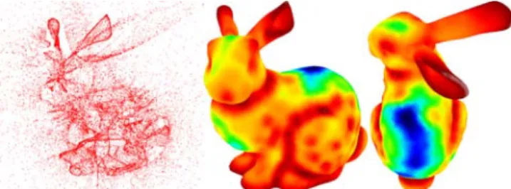
Discrete Skeleton Once the control mesh has been generated, we extract itspolesby selecting a subset of Voronoi vertices (i.e., circumcenters of tets) in the following manner. For each Delaunay vertexvwe first select as a pole the farthest circumcenter from all incident tets. The vector formed byvand this pole is considered as

the local normal estimate. We deduce a local tangent plane estimate inv, and two half-spaces bounded by this plane. Next we search in the half-space that does not contain the pole the farthest Voronoi vertex incident to the site. If it exists it is added as a pole too. We refer the reader to [Amenta and Bern 1998] for a more detailed de-scription of this simple procedure. By definition, and assuming a sufficiently dense set of points sampled on the boundary, the result-ing set of all these poles is a discrete approximation of theskeleton

(or medial axis) of the domain boundary∂Ω(see Fig.7).

Figure 7: Poles: The set of all poles (depicted as red dots) represents a discrete approximation of theskeletonof a 2D (left) or 3D (right) shape.

Local Feature Size At each vertex of the boundary∂Ω, we approximate its local feature sizelfsby measuring the distance to its closest pole (Fig.8). To improve the efficiency of these queries (the set of poles is a dense point set for a complex boundary), we create a static kD-tree search data structure from the poles.

Figure 8: Left: poles extracted from the Bunny model. Middle, right: the distance from each input vertex to the set of poles is the approximatedlocal feature size, capturing both local thickness and curvature of the shape.

Boundary Supersampling The input boundary is initially sampled with a large number of quadrature samples(used later on to find a good approximation of the surface). More precisely, three sets of quadrature samples are generated: on the boundary it-self, on its sharp creases, and on its corners (for piecewise smooth domains—see, e.g., Fig.16); this will allow us to both approximate the boundary and fit its features. Each quadrature sample stores its positionxas well as a quadrature value, incorporating the areads (for surface quadrature samples) or lengthdl(for feature quadrature samples) it covers. These values are set tods/µ(x)4_anddl/µ(x)3 respectively, to conform to our mass density field [Du and Wang 2003]. Each corner sample is given an infinite density to guarantee that a vertex will be assigned there.

3.3 Fast Marching Construction of Sizing Field

Recall that a parameterKis used to adjust the sizing field accord-ing to the desired mesh gradation (see Section2.3, and Figure9

for illustration). We store the sizing field on a uniform grid bound-ing the domain. Each node of the grid must store the local sizbound-ing field valueµand an additional bit to specify whether this grid node lies inside or outside the domain as these grid nodes will be used to efficiently generate initial positions for the vertices of the mesh. However, computingµin the interior ofΩwould require the evalu-ation of a minimum overeachvertex of∂Ω. To provide a faster grid initialization we use a fast marching method on the uniform grid us-ing the 6-neighborhood incidence relationship beginnus-ing with the grid cells that intersect∂Ω. We define acandidate cellxas a cell for which we have stored a temporarybuddy cell, denoted hereafter

y(x). The latter is astride of the boundary, and has the property that

the sizing fieldµ(x). The candidate cells are maintained in a prior-ity queue ordered by their current estimated value ofµ. This queue is initialized with all grid cells that are neighbors of a grid cell in-tersecting∂Ω. At each step of the marching process we pop the candidate cell with minimumµvalue out of the queue, set its final sizing field value toµ, and push other possible adjacent candidates in the queue with the same buddy cell. This fast marching method will thus propagate values ofµfrom the initial boundary to the in-side of the domain. Note that this could introduce an approximation in the evaluation of the sizing field, since the boundary cellc(x) such thatK d(x, c(x)) +lfs(c(x))is globally minimal might not be among the buddy cells ofx’s neighbors. We argue that the error is negligible. The reason is that the set of pointspthat have a same buddy cellyis star-shaped aroundy. Indeed, on the line segment frompto y(p), the function λ(s) = K d(s, y(p)) +lfs(y(p)) decreases with speedK; asµisK-Lipschitz, we have thatλ≤µ, thereforeλ = µsinceµis the minimum over ally ∈ ∂Ω, and finallyy(s) = y(p). Hence, the first grid cellqmet by the ray p−y(p)is most likely such thaty(q) = y(p). One then has

µ(q)≤µ(p); thus,µ(q)must have been already computed by the timepis taken care of. This simple procedure enables an efficient and robust initialization of our sizing field grid.

Figure 9: Sizing fields computed for three increasing values forK_{. The} smallerK_{, the smoother the grading. For large values, the ideal edge size} is rapidly increasing as one moves away from the boundary.

3.4 Initial Point Sampling

Given the potential complexity of the input boundary and the opti-mized 3D Delaunay triangulation in terms of geometry and topol-ogy (with possibly multiple connected components and holes), a good initialization of the tet mesh vertices is desirable. We “spread” the requested number of vertices throughout the domain while roughly matching the desired local density through error diffusion over the sizing field. This initial sampling proceeds in two passes. In order to calibrate the sampling so as to fit the vertex budget spec-ified by the user, the first pass sums up the valuesdv/µ(x)3 for each interior node of the sizing field grid, wheredvdenotes the volume of the node andxits position. The second pass iterates over the same grid nodes in serpentine order, computing for each node its corresponding (floating point) number of initial vertices to lay down locally, quantizes this number to the nearest integer and diffuses the corresponding residual to its neighbors: this process is a straightforward extension of [Ostromoukhov 2001] to volumetric images. Although these placements do not guarantee any quality on the resulting Delaunay mesh, we achieve a local density of vertices consistent with the sizing field for a very low computational effort.

3.5 Energy Minimization

The energy minimization phase, alternating connectivity and ge-ometry optimization, is the core of our algorithm. From the current vertex positions, the energy is minimized by computing the 3D De-launay triangulating of these sites. For a given connectivity, the energy is further minimized by moving eachinteriorvertexxito

its optimal placement within its 1-ring (Eq.8).

Boundary Vertices We must treat the current boundary vertices differently to provide adequate boundary conditions to our mini-mization, as well as a good isotropically-sampled approximation of the domain boundary. A simple and practical solution is to use a

variant of the constrained centroidal Voronoi tessellation approach (CCVT [Du et al. 2003]). First, in order to identify the current boundary vertices, we examine each boundary quadrature sample si, and locate its nearest vertex in the current mesh (through a fast

kD tree query), and accumulate at that vertex the quadrature value atsitimes the coordinates ofsi. Subsequently, we focus on the

ver-tices with a non-zero quadrature sum, since those are the boundary vertices that require a specific treatment. We move these bound-ary vertices to the average value they each have accumulated dur-ing the pass over all quadrature samples. This position provides a good, low-cost approximation of thecentroidof the intersection between the 3D Voronoi cell of the boundary vertex and the input boundary∂Ω. We proceed similarly for the feature quadrature sam-ples involved in the piecewise smooth case, where we must fit sharp creases too. As demonstrated in our results (see Fig.10for an illus-tration of several steps of optimization on a simple boundary), this simple procedure results in well-shaped triangles that fit the domain boundary, and whose size is in agreement with the sizing field.

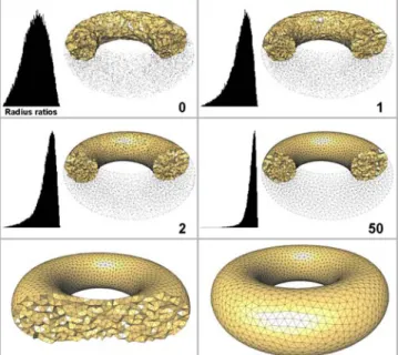
Figure 10:Optimization steps for1000vertices in a torus.100K_quadrature samples were spread on the boundary, and the sizing field is constant to get a uniform mesh. Observe how the radius ratio distribution shifts towards1. 3.6 Accelerating Convergence

Although our quadratic energy minimization provides a powerful tool to design high-quality meshes, the convergence rate can be slow for large number of vertices. We have successfully experi-mented with the following practical shortcuts to get faster results. Delaunay Refinement Direct minimization of more than

100,000vertices can be computationally expensive. Instead, we prefer starting the energy minimization with a much smaller num-ber of vertices. Before it even reaches a minimum, we increase the number of vertices by adding a specified fraction (typically,50%) of the vertices at a subset of the Voronoi centers of the current mesh. To select the latter subset, we sort all tets by decreasing size of cir-cumradius divided by the local desired edge length (to know where refinement is most needed). After another round of minimization steps, we repeat this procedure, until the requested number of ver-tices is reached. The speed-up is considerable, while achieving the same final quality.

Selective Optimizations A straightforward improvement of vertex position update optimizesonlythe vertices adjacent to bad quality tets (say, with a radius ratio less than0.3) and their imme-diate neighbors. Although no theoretical guarantees back up this

trick, it works remarkably well in practice. We recommend switch-ing to such a selective optimization once the full-blown optimiza-tion steps are relatively small in amplitude.

Boundary Vertex Jittering As expected from our energy, the inside tets are well shaped after minimization. However, because of the boundary constraints that we must satisfy, a few slivers can re-mainadjacentto boundary vertices. We have implemented a fast ”jittering” of these points; in order to snap a sliver, we slightly move one of its adjacent boundary vertices in the local tangent plane. Similar in spirit to the more general procedure of sliver exudation [Cheng et al. 1999], but for the easier case of tets on boundaries, this jittering suffices to remove the remaining slivers. Vertex Teleportation or Insertion We also recommend spo-radically removing the vertex with the smallest Voronoi cell w.r.t. the desired edge length (i.e., in the densest region), and inserting it at the centroid of the interior tet with the worst radius ratio. Such tunnelling of vertices is particularly useful when tight control over the worst element is required. If the vertex budget does not have to be maintained, one can directly add vertices inside the worst tets.

Figure 11:Final Extraction: As the Delaunay triangulation covers the con-vex hull, the last stage of our algorithm must extract the inside tets. 3.7 Final Mesh extraction

To produce the final mesh, we need to peel off the Delaunay tets of our mesh that are outside the domain (remember that a Delaunay mesh triangulates the convex hull of the vertices—see Fig.11). A first approach is to consider the Delaunay triangulation restricted to the input domain, by tagging a tet asoutsidewhen its circumsphere center is located outsideΩ. Similar in spirit to the Cocone algo-rithm [Amenta et al. 200], we consider instead the Delaunay trian-gulation restricted to a slightlythickerversion of the input domain

Ω. For each tet initially tagged outside, we compute the ratio be-tween the distancedfrom the circumsphere center to the boundary

∂Ωand the circumradius; if this ratio is smaller than a predefined threshold (0.4in all our experiments) we tag the tet inside.

4 Results and Discussions

The figures in this paper illustrate the robustness and versatility of our technique: our implementation can handle large and/or complex domains of arbitrary topology in a matter of minutes. Although a visual inspection cannot provide a thorough assessment of our re-sults, all the cutaway views as well as the radius ratio distributions that we obtained exhibit high quality tet shapes throughout the do-main. In contrast to many other methods wedo nota priori assign vertices to be either on the boundary or in the interior. It is the min-imization procedure that will make them stick to boundary or not, driven by the sizing field and number of vertices required. This fea-ture partially explains the quality of the results, since the mesh is not constrained to a given budget of boundary vertices. Also, our expe-rience shows that global optimization of the connectivity through a Delaunay triangulation renders the results significantly better: this handling of the connectivity is possibly the sharpest departure from common approaches that perform local updates only.

Results can be obtained in a matter of seconds or minutes. For in-stance, Fig.10was obtained in16seconds (for the50iterations, which include a Delaunay triangulation and the vertex position op-timizations ateachiteration) on a Pentium IV 3GHz. A more com-plex model, such as the hand in Fig. 12requires on average2.1

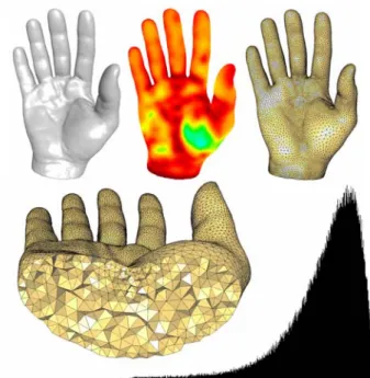
Figure 12: Scanned hand: on this highly detailed mesh (36K _vertices,

174K_{tets, with color-codedlfs), mesh gradation is a must: a uniform mesh} fine enough to capture the surface details would have millions of tets; In-stead, our algorithm can reproduce all the fine surface features while using large tets inside the domain. Sizing field parameter:K= 1. As the radius ratio distribution shows, there are no degenerate tets. Worst radius ratio = 0.29_{, average radius ratio}= 0.86_{, average dihedral angle =}70o_{. Mean}

symmetric distance from input boundary: 0.024% of the bounding box. seconds per iteration, including Delaunay triangulation, boundary quadrature, and vertex updates for the 36K vertices. For good meshes,10to20iterations are sufficient, but we often increase this number to50, and use the speed-ups described in Section3.6for a final high quality result. Although very few timings are available for previous optimization methods, we consider the time involved in our technique for mesh design practical. Notice that we can also deal with sharp features, as Figure16demonstrates—a full treat-ment treattreat-ment of such mechanical would however require a good Constrained Delaunay mesher.

Figure13demonstrates the quality of approximation of the bound-ary for the Bunny model, for increasing vertex budgets ranging from 1K to 10K vertices. We plot the mean symmetric (L2₎ dis-tance in percentage of the bounding box against the number of sites, as well as a color-coded illustration of the approximation error. Judging the quality of the results is, however, a difficult task. First, many (often contradictory) quality measures have been proposed over the years. Second, when averages of radius ratios are given, they do not tell the whole story: many slivers can be present even when the average is high. Finally, we could not find or get tet

Figure 13:Mean symmetric approximation error against the number of sites measured with Metro. The approximation error is expressed in percentage of the bounding box. The four bunnies shown correspond respectively to 2, 4, 6 and 8K sites, with their approximation error in false colors.

Figure 14:Gargoyle: a comparison with [Cutler et al. 2004] gives further evidence of the quality of our results. Our distribution in terms of radius ratios (one of the fairest measures [Shewchuk 2002a]) is far superior to a standard optimization technique (mesh courtesy B. Cutler).

meshes of usual CG models (such as the bunny) or of canonical shapes, aside from the results presented in [Cutler et al. 2004] (see Fig.14for comparison). nevertheless, we provide typical numbers of our results in Table1for comparative purposes. The distribution curves given in most of our figures also indicate how well shaped most of the tets are. We also indicate relevant numbers in each caption for completeness.

Finally, in Fig.15we compare our optimization technique with the unit-mesh approach [Frey and George 2000] used in commercial meshers. This technique has been applied on a high-quality uniform input boundary mesh of the bunny generated using the technique presented in [Surazhsky et al. 2003], resulting in 275K tets and 49K vertices in 12.5s (the number of vertices cannot be specified and results from the conforming of the boundary). As this unit-mesh approach splits long edges into smaller equal-length edges during the meshing process, the final mesh exhibits directional aliasing in the form of lines of tets, potentially detrimental to the simulation of isotropic phenomena. To provide a fair comparison, we used our technique with a uniform sizing field and the same number of final vertices. Our mesh was obtained in 4 min. Both distributions of radius ratios show no slivers; however, our approach yields better shaped tets overall, albeit at the price of a higher cost.

Limitations Our design choice to approximate the input bound-ary instead of conforming to it can also be seen as a limitation for certain applications. Additionally, we do not have theoretical bounds on the quality measures of the resulting tets. However, our results indicate that in practice, our minimization procedure gener-ates well-shaped tets inside the domain, with better radius ratio dis-tribution curves than any of the tet meshes we came across. Note that this high quality, most desirable for simulation purposes, natu-rally comes with higher computational cost than typical greedy (e.g.

Delaunay refinement) methods.

5 Conclusions

We have introduced a novel approach to the construction of high-quality, isotropic tetrahedral meshes. Based on a sound variational

Model #v #tets min/average L2

radius ratio error (%bb)

Torus 1K 4K 0.42 / 0.88 0.17

Bunny 49K 275K 0.37 / 0.89 0.04

Hand 36K 174K 0.29 / 0.86 0.024

Gargoyle 50K 260K 0.23 / 0.88 0.053

Fandisk 3K 14K 0.29 / 0.87 0.021

Table 1:Min/average radius ratios and mean approximation errors of the input boundary obtained on a series of models. “Bunny” refers to Fig.15

principle, our technique provides a robust mesh design tool that can accommodate requirements on the final number of vertices and on the mesh gradation, for arbitrary domain complexity and topology. We demonstrated the scalability of our approach by meshing large, complex domains, even with sharp features. In future work, we wish to explore how to extend our approach to anisotropic meshing using not just a mass density, but a tensor field. Other boundary conditions for our optimization could also be studied.

Acknowledgments The authors wish to thank Peter Schr ¨oder as one of the instigators of this project. Many thanks to Alexandre Olivier-Mangon and George Drettakis for providing us with the torso model. Our gratitude also goes to Joe Warren, Sean Mauch, Peter Krysl, Fehmi Cirak and Tamer, Barbara Cutler, Steve Oudot, Sylvain Pion, and Andreas Fabri for precious help along the way. Sponsors include NSF (CARGO DMS-0221669 and DMS-0221666, CAREER CCR-0133983, and ITR DMS-0453145), DOE (DE-FG02-04ER25657), the EU Network of Excel-lence AIM@SHAPE (IST NoE No 506766), and Pixar.

References

AMENTA, N.,ANDBERN, M. 1998. Surface Reconstruction by Voronoi Filtering. In Proc. of14th_{Symp. on Computational Geometry (SCG’98), 39–48.}

AMENTA, N., CHOI, S., DEY, T.,ANDLEEKHAU, N. 200. A Simple Algorithm for Homeomorphic Surface Reconstruction. InProceedings of the Symposium on Computational geometry, 213–222.

BOISSONNAT, J.-D.,ANDOUDOT, S. 2005. Provably Good Sampling and Meshing of Surfaces.Graphical Models (special issue on Solid Modeling). To appear. BOROUCHAKI, H., GEORGE, P., HECHT, F., LAUG, P.,ANDSALTEL, E. 1997.

Delaunay mesh generation governed by metric specifications. Part 1 : Algorithms. Finite Elements in Analysis and Design 25, 61–83.

BOROUCHAKI, H., GEORGE, P.,ANDMOHAMMADI, B. 1997. Delaunay mesh generation governed by metric specifications. Part 2 : Application examples.Finite Elements in Analysis and Design 25, 85–109.

CAREY, G. F. 1997. Computational Grids: Generation, Adaptation, and Solution Strategies. Taylor & Francis eds.

CHEN, L.,ANDXU, J. 2004. ”Optimal Delaunay triangulations”.Journal of Compu-tational Mathematics 22, 2, 299–308.

CHEN, L. 2004. Mesh smoothing schemes based on optimal Delaunay triangulations. InProceedings of 13th International Meshing Roundtable, 109–120.

CHENG, S. W.,ANDDEY, T. K. 2002. Quality meshing with weighted Delaunay refinement. InProc.13th_{ACM-SIAM Sympos. Discrete Algorithms, 137–146.} CHENG, S.-W.,ANDPOON, S.-H. 2003. Graded conforming Delaunay

tetrahedral-ization with bounded radius-edge ratio. InProc, of the14th_ACM-SIAM Sympo-sium on Discrete algorithms (SODA), 295–304.

CHENG, S.-W., DEY, T. K., EDELSBRUNNER, H., FACELLO, M. A.,ANDTENG, S.-H. 1999. Sliver Exudation. InProc. 15th ACM Symp. Comput. Geom., 1–13. CHENG, S.-W., DEY, T. K., RAMOS, E.,ANDRAY, T. 2004. Quality Meshing for

Polyhedra with Small Angles. InProc. of ACM Symp. on Comp. Geom., 290–299. COHEN-STEINER, D.,DEVERDIERE, E. C.,ANDYVINEC, M. 2002. Conforming

Delaunay triangulations in 3D. InProc. of Symp. on Comp. Geom., 237–246. COHEN-STEINER, D., ALLIEZ, P.,ANDDESBRUN, M. 2004. Variational Shape

Approximation.ACM Trans. on Graphics (SIGGRAPH), 905–914.

CUTLER, B., DORSEY, J.,ANDMCMILLAN, L. 2004. Simplification and Improve-ment of Tetrahedral Models for Simulation. InProceedings of the 2004 Eurograph-ics/ACM SIGGRAPH Symposium on Geometry Processing, 95–104.

Figure 15:Comparison of our method (right, obtained in 4 minutes) with the unit mesh approach [Frey and George 2000] (left, obtained in 12 seconds). To make a fair comparison we provide as input a uniform mesh and specify a uniform density for both methods. The distribution of radius ratios (middle) demonstrates the quality of our resulting tetrahedra.

DU, Q.,ANDWANG, D. 2003. Tetrahedral mesh generation and optimization based on centroidal Voronoi tessellations.International Journal on Numerical Methods in Engineering 56(9), 1355–1373.

DU, Q., GUNZBURGER, M.,ANDJU, L. 2003. Constrained Centroidal Voronoi Tessellations for Surfaces.SIAM J. Sci. Comput. 24, 5, 1488–1506.

EPPSTEIN, D., 2001. Global optimization of mesh quality. Tutorial at the10th_Int. Meshing Roundtable, Newport Beach.

FABRI, A., GIEZEMAN, G.-J., KETTNER, L., SCHIRRA, S.,ANDSCHONHERR¨ , S. 2000. On the Design of CGAL, a Computational Geometry Algorithms Library. Softw. – Pract. Exp. 30, 11, 1167–1202. www.cgal.org.

FREITAG, L.,ANDOLLIVIER-GOOCH, C. 1996. A comparison of Tetrahedral Mesh Improvement Techniques. InProc. of 6th Int. Meshing Roundtable, 87—1000. FREY, J. L.,ANDGEORGE, P. L. 2000. Mesh Generation: Applications to Finite

Elements. Herm`es, Paris.

HARDIN, D. P.,ANDSAFF, E. B. 2004. Discretizing Manifolds via Minimum Energy Points.Notices of the AMS 51(10), 1186–1194.

HOPPE, H., DEROSE, T., DUCHAMP, T., MCDONALD, J.,ANDSTUETZLE, W. 1993. ”Mesh Optimization”.ACM Trans. on Graphics (SIGGRAPH), 19–26. KRYSL, P.,ANDORTIZ, M. 2001. Variational Delaunay Approach to the Generation

of Finite Element Meshes.Int. J. for Num. Meth. in Eng. 50(7), 1681–1700. LI, X.-Y.,ANDTENG, S.-H. 2001. Generate Sliver Free Three Dimensional Mesh.

InProc.12th_{ACM-SIAM Sympos. Discrete Algorithms.}

LI, X.-Y., TENG, S.-H.,ANDUNGOR, A. 2000. ”Biting: Advancing Front Meets Sphere Packing”.Int. J. on Num. Methods in Eng. 49, 1, 61–81.

LLOYD, S. P. 1957. Least Squares Quantization in PCM’s. Tech. rep., Bell Telephone Laboratories, Murray Hill, NJ.

MITCHELL, S.,ANDVAVASIS, S. 2000. Quality Mesh Generation in Higher Dimen-sions.SIAM J. Sci. Comput. 29, 1334–1370.

MOLINO, N., BRIDSON, R., TERAN, J.,ANDFEDKIW, R. 2003. A Crystalline, Red Green Strategy for Meshing Highly Deformable Objects with Tetrahedra. In Proceedings of the 12th International Meshing Roundtable, 103–114.

OSTROMOUKHOV, V. 2001. A simple and efficient error-diffusion algorithm. In Proceedings of ACM SIGGRAPH, 567–572.

OWEN, S. J. 1998. A Survey of Unstructured Mesh Generation Technology. In Proceedings of the 7th International Meshing Roundtable, 239–267.

QUADROS, W. R., SHIMADA, K.,ANDOWEN, S. J., 2004. 3D Discrete Skeleton Generation by Wave Propagation on PR-Octree for Finite Element Mesh Sizing. Poster, Solid Modeling Conference.

RUPPERT, J. 1993. A New and Simple Algorithm for Quality 2-Dimensional Mesh Generation. InProc. of the4th_{ACM/SIAM Symp. on Disc. Algo. (SODA), 83–92.} SHEWCHUK, J. R. 1998. A Condition Guaranteeing the Existence of Higher-Dimensional Constrained Delaunay Triangulations. InProc.14th _{Annu. ACM} Sympos. Comput. Geom., 76–85.

SHEWCHUK, J. R. 1998. Tetrahedral mesh generation by Delaunay refinement. In Proc. 14th Annu. ACM Sympos. Comput. Geom., 86–95.

SHEWCHUK, J. 2002. What Is a Good Linear Element? Interpolation, Conditioning, and Quality Measure. InProc. of11th_{Int. Meshing Roundtable, 115–126.} SHEWCHUK, J. R. 2002. Delaunay Refinement Algorithms for Triangular Mesh

Generation.Computational Geometry: Theory and Applications 22, 21–74. SURAZHSKY, V., ALLIEZ, P.,ANDGOTSMAN, C. 2003. Isotropic Remeshing of

Surfaces: a Local Parameterization Approach. InProc. of12th_{Int. Meshing} Roundtable.

TENG, S.-H., WONG, C. W.,ANDLEE, D. T. 2000. Unstructured Mesh Generation: Theory, Practice, and Perspectives.International Journal Computational Geometry and Applications 10, 3 (June), 227–266.

WARREN, J., SCHAEFER, S., HIRANI, A.,ANDDESBRUN, M., 2004. Barycentric Coordinates for Convex Sets. Preprint.

A Lipschitz Sizing Field

We wish to prove that the sizing field defined in Eq. (9) is bothK-Lipschtiz and maxi-mal. Because we want the function to beK-Lipschitz and agree withlfson the bound-ary, one can easily show the following property:

µ(x)≤ inf

s∈∂Ω

[K d(x, s) +lfs(s)].

We now need to show that the rhs is K-lipschitz and coincides with thelfson the boundary: if so, the rhs will be the maximal sizing field we seek.

Forx∈Ω, let y(x) =argmins∈∂Ω[K d(x,s) +lfs(s)]. Ifx0is inΩ, we have by definition: µ(x0) ≤ K d(x0, y(x)) +lfs(y(x)) ≤ K d(x0,x) +K d(x, y(x)) +lfs(y(x)) ≤ K d(x0,x) +µ(x)

Figure 16:Mechanical parts: Even in the presence of sharp features, our tet meshing algorithm exhibits excellent behavior for low or high vertex count while capturing features and corners remarkably well. We tagged edges as sharp features if their dihedral angles are more than20o_—more

sophisti-cated segmentation techniques could of course be used. (Top, middle) Joint model (1.2K_{vertices); (Bottom) Fan disk model (}3K_{vertices, mean/max} symmetric distance from input boundary: 0.021%/0.5% of the bounding box), along with its radius ratio distribution. Notice the good aspect ratio of both tets (see cutaway views) and surface triangles. A constant sizing field has been used for both models to obtain uniform tet meshes. which shows thatµisK-Lipschitz. Sincelfsis 1-Lipschitz,

we cannot hope thatµcoincides withlfson∂ΩunlessKis at least 1. If so, then forx∈∂Ωwe have

K d(x,y) +lfs(y)≥lfs(x)

for ally ∈∂Ω, with equality wheny= x. Thus,µdoes

coincide withlfson∂Ω. Note that whenK= 1,µ(x)boils down to the length of the shortest path fromxto the medial axis of∂Ωwhile passing by a point on∂Ω. When

Kis less than 1, we get thatµ(x)can be less thanlfs(x)on the boundary due to the Lipschitz constraint; however, the gradation is respected and the boundary sampling will be better than what is necessary: it is therefore still a good choice of sizing field.

B Transforming the Energy

E

Let us start with the definition:

EODT=||f−f_PWLprimal||L1= X j Z Tj |f−f_PWLprimal|. (10) In the tetTjwith verticesxii= 1. . .4, the error function can be expressed as a function of the barycentric coordinatesλi(x):

|f(x)−f_PWLprimal(x)|= X i λi(x)x 2 i−x 2 =X i λi(x) (xi−x) 2 . (11)

Notice that Eq. (3) is easily derived from this last expression by plugging it into Eq. (10). Rewritingxi−xas((xi−cj) + (cj−x)), wherecjis the circumcen-ter ofTj, and plugging it into Eq. (10), we get the following confirmation of Eq. (7):

EODT= X j Z Tj R2j−||x−cj|| 2 dx=X j |Tj|R 2 j− Z Tj ||x−cj|| 2 dx .

C Updates as Weighted Circumcenters

cT. As a consequence, the optimal position of a vertex that has only four neighbors is exactlyatcT. Using Eq. (5) in this special case of a 1-ring in the shape of a tet

T= (xp,xq,xr,xs), and taking the pointxito be located onxp, we get:

cT =xp− 1 2|Ωi| ( ∇x_p|T|) h P x k∈T ||xp−xk|| 2i + F(xp,xq,xr) +F(xp,xq,xs) + F(xp,xr,xs) ) where the extra terms on the rhs only depend on each face of the tet. Applying this formula to an arbitrary 1-ring centered onxp, the face terms cancel each other if we sum the contributions from all the tets, simplifying the expression drastically, and resulting in Eq. (6).