Appendix
Appendix A: Acquiring EPR Spectra and Optimizing Parameters
This appendix provides a step-by-step guide for obtaining an EPR spectrum and optimizing parameters, using Bruker software. The proper user-selected spectrom-eter settings (as discussed in detail in Chap. 4) are key to obtaining spectra that allow for accurate peak height measurements or double integrations. Selection of parameters for Tempol (4-hydroxy-2,2,6,6-tetramethylpiperidine-1-oxyl) is used as the example because it is a convenient reference standard for measurements involving various spin trap and spin label nitroxides. Remember that for quantita-tion the standard and the unknown should be dissolved in the same solvent, contained in the same size tube, and positioned similarly in the same resonator.Measure the Spectrum with Nominal Settings
l Microwave power 5 mW l Modulation amplitude 1 G l Field sweep 200 G
l Scan time 5.1 s (if the sample is very weak, the scan time or gain may be increased) (Fig.A.1)
Optimize the Microwave Power
The microwave magnetic field (B1) is what causes the EPR transition in the sample
(see Chap. 6). B1is proportional to the square root of the microwave power output
by the bridge. The “effective” intensity of B1 over the sample depends on the
incident microwave power, on the type of cavity or resonator that is used, and on the length of the sample. Therefore the power saturation behavior of a sample is determined experimentally. Figure A.2 shows the dependence on square root of the microwave power for the double integral (top curve), as well as the peak-Fig. A.1 Measuring the initial EPR spectrum
to-peak height (a power saturation curve) and line width (bottom curves) for a rapidly tumbling Tempol sample. Most power saturation curves show a linear region (non-saturating) at low microwave power and a nonlinear region (saturating) at higher microwave power. In the region where the signal does not increase linearly with square root of power, the double integration increases nonlinearly and the linewidth increases. These data provide the basis for selecting instrument parameters for different experiments. For example, to simply maximize the signal intensity of a very weak sample for which power saturation is not of concern, a higher power level can be selected. However, if spectra will be used to characterize hyperfine splittings or line widths, a power in the non-saturating region should be selected. To quantitate the concentration of a sample using peak heights or double integrals, the spectra of both the sample and the spin standard should be measured under nonsaturating conditions. For Tempol in a TE102 cavity the maximum
1.0 0.8 0.6 0.4 0.2 0.0 100 80 60 40 Normalized Changes Double Integration 20 0 – 2 0 2 4 6 8 10 12 14 16 – 2 0 2 4 6 SQRT (Power, mW) SQRT (Power, mW)
Line width change (%) Peak-to-peak height
(normalized to 100)
8 10 12 14 16
Fig. A.2 Effect of microwave power on the double intregral, peak-to-peak height, and linewidth of the nitroxide Tempol in water using an ER 4103TM cavity
microwave power in the linear region is about four to five mW (Fig.A.2). Many organic radicals and spin adducts have power saturation curves in the same resona-tor that are similar to Tempol.
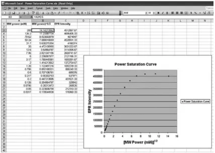
To select the appropriate power for a sample, first perform an automated 2D power sweep experiment, which records field sweeps at a series of microwave powers. The example in Fig. A.3 has a starting power of 200 mW (full leveled power) and successive scans at lower powers (i.e., 2 dB steps):
l Configure the power sweep experiment and collect the spectra l Use the peak intensity (height) data to plot the power saturation curve l Choose a microwave power level appropriate for the experiment
l To calculate spin concentration, choose a power level that is well within the linear region of the power saturation curve (e.g.,2 mW for the case shown in Fig.A.4).
l If the signals are weak and relative intensity measurements for samples with the same power saturation characteristics are adequate, a higher microwave power that provides improved signal-to-noise can be chosen.
Optimize the Modulation Amplitude
Field modulation amplitude also affects the line width and the peak-to-peak height. The data in Fig.A.5show that as the modulation amplitude is increased, the line width remains constant to a point, after which it broadens.
The natural line width (Fig.A.6) of the signal can be estimated by measuring the spectrum with increasing modulation amplitude until the spectrum starts to broaden. Then make additional measurements at successively lower modulation amplitude values until the line width no longer gets smaller. The measured line width is then very close to the natural line width. If accurate lineshapes or resolution of small hyperfine splittings are important, the modulation amplitude should be less than 1/10 the natural linewidth. If the signal-to-noise is poor, it can be improved at the expense of linewidth accuracy (see Sect. 4.11). To maximize the signal-to-noise, the modulation amplitude can be set as high as about 1.5 times the natural line width. So, for example, if the natural line width is 1.7 G one might use 2.5 G modulation amplitude. The broadening of the signal by high modulation amplitude is called “over-modulation.”
FigureA.7shows the changes of peak-to-peak height of the Tempol signal with increasing field modulation amplitude. For Tempol the maximum peak-to-peak height is observed when the modulation amplitude is about 1.7 times the natural line width. Higher modulation amplitudes cause the peak height to decrease. Even for modulation amplitudes that are so large that the peak-to-peak height decreases, the double integration increases linearly with modulation amplitude (see Fig.A.8). This means that overmodulation of the signal can be used for quantitative compar-isons of double integrals, provided that the field scan range is wide enough to accommodate the broadened spectrum.
Optimize Magnetic Field Sweep Width and Number of Data Points
EPR lines often extend further into the outer regions of the spectrum than estimated at first glance. Therefore, it is important to use a magnetic field sweep width that is wide enough to encompass the entire spectrum. This effect is particularly important for the double integrations that are needed for signal quantitation. FigureA.9shows Fig. A.3 Parameters and spectra for the automated power sweep experiment
the dependence of the double integral on sweep width. If the sweep width is not wide enough, a considerable portion of the spectrum is missing from the double integration. A good “rule of thumb” for Gaussian lines is to use a sweep width such that the distance between the first field value in the sweep and the start of the EPR signal is ten times the peak-to-peak linewidth of the narrowest signal (see “A value” in Fig.A.9).
So, for example, if the line width is 2.8 G, the field sweep should begin at least 28 G before the first line. If the line is Lorentzian, data extending for 30 linewidths Fig. A.4 Plotting the power saturation curve
1.2 1.0 0.8 0.6 0.4 0.2 0.0 0 1 2
Modulation Amplitude / Line Width
Line Width Changes
/Line Width
3 4
Natural line width = 1.7 gauss Over-modulated Line width = 2.8 gauss a b
Fig. A.6 Measurement of the natural line width of the spectrum with a cursor tool in the acquisition software. Window A shows a modulation setting that provides a spectrum with the sample’s natural line width. Window B shows a higher modulation amplitude setting and a slightly over-modulated spectrum 1.6 1.4 1.2 1.0 0.8 0.6 0.4 0.2 0.0 0 1 2 3
Modulation Amplitude / Natural Line Width
Peak-to-Peak Height
4 5 6 7
Fig. A.7 Changes in the peak-to-peak height of the Tempol signal with increasing modulation amplitude
is required for accurate integration (Fig.A.10). It is advisable to be conservative and perform a very wide sweep that assures all of the data from the EPR absorption is collected. Also, be sure that the number of data points is large enough that there are at least ten data points to define the peak-to-peak linewidth of the narrowest signal.
Summary
Configuring the spectrometer for quantitative experiments usually requires a com-promise between settings that optimize the signal-to-noise, yet provide reproduc-ible and fair comparisons between the reference standard and the unknown sample.
7 6 5 4 Double Integration 3 2 1 0 0 1 2 3 Bmod/DBp-p 4 5 6 7
Fig. A.8 The double integral of the Tempol signal increases linearly with modulation amplitude 0.9 0.8 0.7 0.6 0.5 0.4 0.3 0.2 0.1 0.0 0 5 10 15 A
Scan Width (A / line width)
Double Integration
20 25 30
So, in summary, for a given amount of spectrum acquisition time, select values for the following parameters:
l Microwave power– to quantitate the spin concentration of a sample using the double integration method, the sample and the spin standard must be measured under nonsaturating conditions. Thus, a microwave power that is well within the linear region of the power saturation curve for the respective sample and standard must be used.
l Modulation amplitude– Since the double integration is proportional to the field modulation amplitude even if the signal is broadened, a relatively high field modulation can be used. In fact, aside from performing longer acquisitions. (e.g., performing long scans or signal averaging) increasing field modulation is the safest way to obtain better spectra of weak signal for double integration. l Sweep width– Field sweep width is another factor that will adversely affect the
double integration if set too low. The optimal sweep width depends on the line shape of the signal, but a safe rule of the thumb is to set the sweep width so that the distance from the field starting position to the first EPR line is ten times the
Over-modulated Line width = 2.8 gauss
Distance to first line = 32 Gauss
Fig. A.10 Measuring the line width and the distance from the first field point to the first EPR line Appendix A: Acquiring EPR Spectra and Optimizing Parameters 123
width of the narrowest line. Frequently the signal averaging method gives a better baseline than a single scan with a long time constant. In any case, it is best to keep the time constant and sweep time the same for the sample and standard. If a larger number of scans is needed for the unknown than for the standard, the double integrals can be divided by the number of scans averaged.
l Maximizing signal intensity– Remember, if the goal is only maximizing signal to noise (and not for quantitation), higher microwave power and field tion amplitude can be used. However, if the microwave power or field modula-tion amplitude is too high the signal intensity may actually decrease. Set the field modulation amplitude at about 1.5 times the line width and the microwave power at the top of the power saturation curve to get the maximum signal intensity. This should give a good signal to noise enhancement although lines will be broadened.
Appendix B: Field Modulation and Phase Sensitive Detection
This appendix provides engineering level detail on how field modulation is used to detect the EPR signal. It can be omitted by readers who are not interested in this level of detail.Details of Field Modulation and Phase Sensitive Detection
The EPR signal at microwave frequencies, such as 9.5 GHz, is “detected” by the crystal in the bridge. The output of the detector crystal is a DC (direct current) signal that is modulated as described in the following paragraph.
DC electronics are often noisy and the low-frequency components of the noise often appear as baseline instability. One common technique to remedy this problem is to modulate and then demodulate. By shifting a low frequency signal to a higher frequency (modulation), amplifying and processing it, and then converting it back into a low frequency signal (demodulation), superior baseline stability and noise reduction are obtained. An example of such a technique would be AM and FM radio. The audio signals are up converted to RF and then down converted to audio frequencies in the radio. An example in an EPR spectrometer is the use of field modulation. The microwave detector output from an EPR absorption is very noisy at low frequencies, but diminishes with 1/frequency as the frequency increases. The EPR signal is shifted to a higher frequency by modulating the magnetic field (often at 100 kHz). The EPR signal is then demodulated in the signal channel to obtain the desired noise-suppressed and stable low frequency EPR signal.
The heart of phase sensitive detection is a mixer. It has two inputs and one output. The output of the mixer is the product of the two input signals. The symbol for a mixer is shown in Fig.B.1. Notice the X which symbolizes multiplication.
IF stands for Intermediate Frequency and is the resulting output signal that is subsequently filtered and processed to produce the EPR spectrum.
Modulation typically is sinusoidal. If a signal described by:
A1cosðo1tþ’Þ (B.1)
is applied to one input of the mixer and a signal described by:
A2cosðo2tÞ (B.2)
to the other input, the the product output signal is described by:
A1cosðo1tþ’Þ:A2cosðo2tÞ (B.3) Using trigonometric relationships, this becomes:
1=2A1A2fcosððo1o2Þtþ’Þ þcosððo1þ o2Þtþ’Þg (B.4)
In this form three salient features of the IF output can be seen:
l The IF output can be decomposed into two frequency components: the sum and difference frequencies of the two input signals.
l The amplitude is equal to one half the product of the amplitudes of the two input signals.
l There is a phase factor,j, equal to the phase difference between the two signals. This is the term that gives the name phase sensitive detection.
It is the sum and difference frequencies that make up and down conversion (or modulation and demodulation) possible. A high or low pass filter can be used to select either the sum or difference frequency component. The amplitude property facilitates the use of mixers for modulation and demodulation as well as feedback
Reference Signal EPR Signal
IF Signal Out Fig. B.1 Schematic of a mixer
loops. The phase factor can be used to discriminate between signals of different phase.
Quite often the LO (reference) input has the same frequency as the signal input and its amplitude is kept constant. The IF output is then zero frequency (DC) and double the frequency. FigureB.2shows the IF output for various phase differences. The dashed lines indicate the DC components. Note the double frequency compo-nent as well.
If the low frequency component is selected by filtering out the high frequencies with a low pass filter, the IF output is proportional to:
A2cosð’Þ (B.5)
This scheme permits measurement of both the amplitude and phase of the input signal. If the input signal amplitudes remain constant, the IF output is proportional to cos(j) and then the mixer functions as a phase detector (Fig.B.3). When the frequency difference and the phase difference between the two signals is zero, the DC output is at a maximum. 0 0 0 0 0 0 0 0 0 0 0° 270° 90° 180° 0 0
Fig. B.2 The IF output for different phase differences
Phase
180° 360°
0
Fig. B.3 The output of a phase detector
Field Modulation and Demodulation
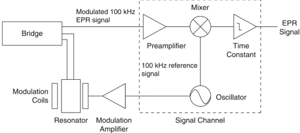
The magnetic field at the sample can be modulated (often at 100 kHz) using the modulation coils (or posts) on the resonator. The resulting modulated signal is then demodulated in the signal channel. A block diagram of the circuitry in an EPR spectrometer for modulation and demodulation is shown in Fig.B.4. The relation-ship between the field modulated signal and the first derivative of the EPR absorp-tion lineshape is depicted in Fig.B.5.
A Visual Description of Why the EPR Signal Appears in the First
Derivative Form
The following figures are used to illustrate how the first derivative spectrum is the resulting output from the signal that is demodulated in the signal channel. The Modulated Signal (Fig.B.6) originates from the reflected microwaves coming from the cavity and is the input to the signal channel. The Unfiltered Demodulated Signal is the phase detected signal before it is filtered by the signal channel. The dashed horizontal line in that display is the average value of the unfiltered signal and is equivalent to the signal after it is filtered by the time constant. The two displays on the left side are the EPR absorption signal and the corresponding phase detected and filtered EPR signal. The vertical dashed line indicates the magnetic field value at a given time in the EPR experiment. The Demodulated Lorentzian display is the phase detected and filtered EPR signal plotted as a function of the magnetic field. In each successive figure, a black dot data point is added to the recorded output spectrum. These data points correspond to the position (or amplitude) of the
Bridge Modulation Coils Modulation Amplifier Signal Channel Oscillator 100 kHz reference signal Modulated 100 kHz
EPR signal EPR
Signal Preamplifier Mixer Time Constant Resonator
Fig. B.4 A simplified diagram showing parts of the EPR spectrometer that are used for field modulation and phase sensitive detection. The microwave EPR signal is converted to a modulated DC signal by the crystal detector in the bridge
horizontal dashed line that is shown in the plot of the “Unfiltered Demodulated Signal.”
If the magnetic field is moved to a position in the EPR signal, an oscillation is observed with amplitude that is approximately proportional to the slope of the signal (Fig.B.7).
Steep Slope = Large Amplitude Shallow Slope = Small Amplitude
Fig. B.5 Conversion of modulation into a modulated signal
Data points in EPR spectrum
Unfiltered Demodulated Signal Modulated Signal Lorentzian Demodulated Lorentzian –10 –5 0 5 10 –10 –5 0 5 10 0 5 10 0 5 10
Field Modulation and Demodulation
Field position far before resonance where slope is very low
Fig. B.6 When the field is at a position far before resonance the slope is near zero and so a baseline data point is recorded
At the top of the EPR absorption, the output of the mixer has twice the modula-tion frequency. This results from the fact that the EPR absorpmodula-tion signal is symmet-ric at that point. The filtered demodulated signal drops to zero here. This data point provides the “zero cross” or baseline value within the EPR absorption envelope (see Fig.B.8).
If the field is shifted further, a 180 phase shift in the modulated signal can be seen by comparing the modulated signals in Figs.B.7andB.9. Also notice that the filtered demodulated signal (the horizontal dashed line) becomes negative after the midpoint of the EPR absorption.
And once again, for a magnetic field that is well past the field for resonance, the slope is very near zero corresponding to a baseline point (see Fig. B.10). For illustrative purposes, only five data points were shown while stepping through this example. FigureB.10shows the actual spectrum that would be obtained with multiple points across the field scan range.
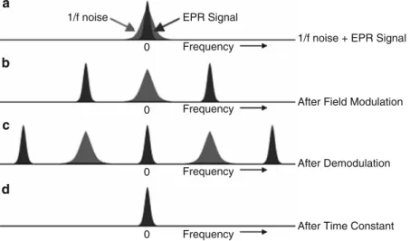
Suppression of 1/f Noise
Another reason for using modulation and phase sensitive detection is to suppress 1/f noise. Noise drops off at higher frequencies. If no modulation is used, the EPR signal has predominately low frequency components. The output of the diode detector is dominated by the 1/f noise and not by the EPR signal (see Fig.B.11a). Data points in EPR spectrum Field position just
before maximum where slope is high Unfiltered Demodulated Signal Modulated Signal Lorentzian Demodulated Lorentzian – 10 – 5 0 5 10 – 10 – 5 0 5 10 0 5 10 0 5 10
Field Modulation and Demodulation
Fig. B.7 Approaching the center of the EPR absorption signal in a region with a high (positive) slope
Data points in EPR spectrum Field position at top of absorption is also zero Unfiltered Demodulated Signal Modulated Signal Lorentzian Demodulated Lorentzian – 10 – 5 0 5 10 – 10 – 5 0 5 10 0 5 10 0 5 10
Field Modulation and Demodulation
Fig. B.8 Signals at the center of the EPR absorption signal
Data points in EPR spectrum Field position just
after maximum where the slope is high Unfiltered Demodulated Signal Modulated Signal Lorentzian Demodulated Lorentzian – 10 – 5 0 5 10 – 10 – 5 0 5 10 0 5 10 0 5 10
Field Modulation and Demodulation
Fig. B.9 Signals on the right side of the EPR absorption, but still in a region with a high (negative) slope
Field position far after resonance where slope is very low Unfiltered Demodulated Signal Modulated Signal Lorentzian Demodulated Lorentzian – 10 – 5 0 5 10 – 10 – 5 0 5 10 0 5 10 0 5 10
Field Modulation and Demodulation
Fig. B.10 Signals for a magnetic field position that is well past resonance, and the lineshape that would be obtained if multiple additional points had been examined
1/f noise
a
b
c
d
1/f noise + EPR Signal
After Field Modulation
After Demodulation
After Time Constant 0 0 0 0 EPR Signal Frequency Frequency Frequency Frequency
Fig. B.11 A cartoon of how field modulation and phase sensitive detection is realized in an EPR spectrometer
If 100 kHz field modulation is applied, the EPR signal is shifted to 100 kHz (see Fig.B.11b). The noise is not frequency shifted because the field modulation only has an effect on anything that is magnetic field dependent such as the EPR signal and not on anything field independent such as the 1/f noise. There is no mechanism for the field modulation to affect the 1/f noise.
The EPR signal is now nicely separated from the 1/f noise, but alas it is at 100 kHz. After phase sensitive detection, our EPR signal is shifted to 0 Hz and 200 kHz (see Fig.B.11c.). The 1/f noise is also shifted to 100 kHz. Unlike in the case of modulation having no effect on the noise, the 1/f noise, like any signal, will exhibit both sum and difference frequencies after demodulation. Finally, the unwanted 200 kHz EPR signal and 1/f noise are filtered out by the RC filter with a selectable time constant (see Fig.B.11d.), and the unwanted 1/f noise has been successfully suppressed.
Appendix C: Post Processing for Optimal Quantitative Results
A user may want to make relative intensity measurements with samples that only provide very noisy spectra or may want to perform double integrations on spectra with background or baseline problems. In such cases, there are a number of post processing procedures that can greatly improve the accuracy and precision of the quantitative EPR measurements. In this appendix two examples are outlined for improving experimental spectra through post acquisition processing.Example of Baseline Subtraction to Improve Spectrum for Double
Integration
Double integration of the first derivative EPR spectrum is used to quantitate EPR samples. Because most spectrometers record the EPR signal as a first derivative of the absorption signal, the spectrum must be integrated once to recover the absorp-tion spectrum and then integrated a second time to obtain the area under the absorption curve. Spectral processing software performs the double integration. The following section demonstrates how to perform double integrations using Bruker’s WIN EPR spectral processing software and also provides suggestions for improving the accuracy of double integrations. WIN EPR is used only as one example; there are many other software programs available that can perform the same tasks.
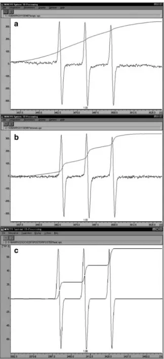
It is important to realize that even slight baseline drifts, background signals, or a very low signal to noise ratio can be detrimental to the accuracy of double tions. Fortunately, there are many tell-tale signs that warn a user of a poor integra-tion. FigureC.1shows how a double integration was improved by signal averaging
Fig. C.1 Spectrum (a) was collected using a 326 ms time constant and a 335 s scan. Spectrum (b) was recorded using a series of 32 scans with a 10.2 ms time constant
Note: The total acquisition times for (a) and (b) were the same. Spectrum (c) is a simulation of the experimental spectrum. Double integrations are overlaid on each spectrum
a series of short scans with a short time constant, or by simulating the experimental spectrum. The double integrations are overlaid on each spectrum. In (a), the double integral curve starts rising long before the EPR signal begins. Although (b) is much improved, the curve still starts to rise before the EPR signal begins. Meanwhile, the double integration of the simulated spectrum (c) has no confounding baseline effects (i.e., only the EPR signal of interest has been calculated).
Seemingly insignificant baseline drifts and/or background signals often have a confounding effect on the double integration of the EPR spectrum. Consider a spectrum that also has an extremely broad background signal. Even though the peak-to-peak height of the background may be so small that it is unrecognizable, its double integrated intensity may be larger than a very narrow signal that dominates the first derivative representation of the spectrum. In Fig.C.2spectra (a) and (b) are Fig. C.2 Improvement of double integration using the baseline fit and subtract feature of WIN EPR. Spectrum (a), is the first derivative spectrum before baseline correction. Spectrum (b), is the first derivative spectrum after subtracting the baseline. The double integrations appear overlaying each spectrum
actually the same EPR spectrum, except in (b), the baseline has been subtracted. The double integrations are displayed overlaying both spectra. Although the first derivative representations seem almost identical, the double integration of the uncorrected spectrum in (a) is distorted. This would, undoubtedly, give a mislead-ing result if it were used in a quantitative study. The followmislead-ing paragraphs demon-strate how post processing software can be used not only to obtain numerical double integration values, but also how to improve the accuracy of these values when the EPR spectrum has an unavoidable background signal or baseline drift.
Convert the First Derivative EPR Spectrum into an Absorption
Spectrum
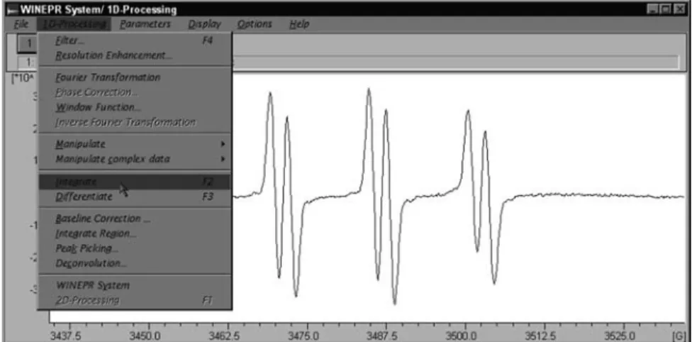
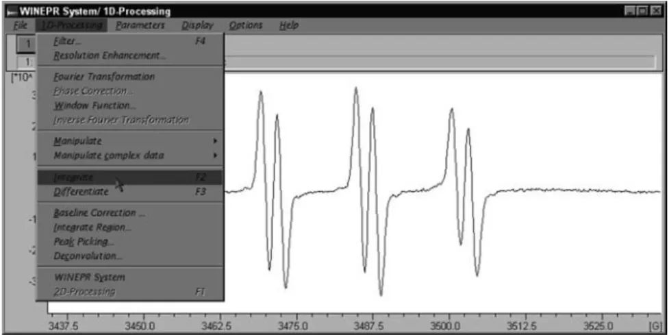
It is often easier to visualize and to correct a distorted baseline when working from the absorption spectrum. To convert the first derivative to an absorption curve, select “Integrate” under the “1D-Processing” menu (Fig.C.3).
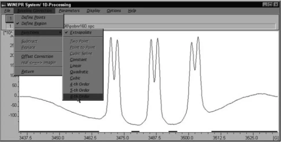
Correct the Baseline
It becomes apparent from the absorption spectrum that the baseline is not flat (Fig.C.4). To calculate the baseline, first select “Baseline Correction...” under the “1D-Processing” drop-down menu. From the “Baseline Correction...” menu, select “Define Region” and define the region of the spectrum. Do this by clicking the left mouse button to designate the starting point of a region. Then drag the pointer to the desired end of a region and click the right mouse button. The regions that were
Fig. C.3 Converting the spectrum to an absorption representation
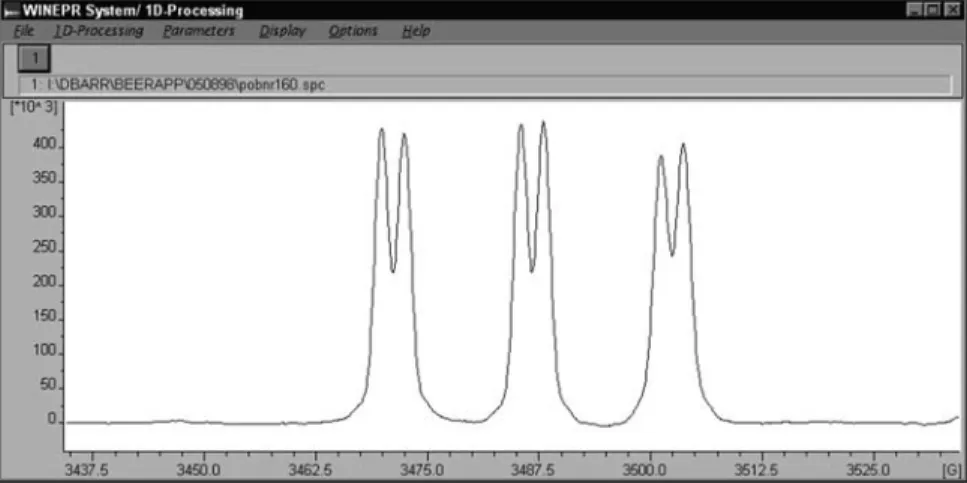
defined for this spectrum are marked with dark colored bars at the bottom of the window (Fig.C.4). It is important not to include any points from the actual EPR spectrum in the region that is defined for baseline correction. After defining the regions, calculate the baseline using a function from the “Functions” menu within the “Baseline Correction...” drop-down menu. In this example a sixth order poly-nomial was selected to calculate the baseline based on the selected regions. The fit of the baseline appears overlapping the spectrum in Fig.C.5. Next, select “Sub-tract” from the “Baseline Correction...” drop-down menu. The absorption spectrum with a corrected baseline then appears (Fig.C.6). At this point, if the user is satisfied with the result, click “Return” which returns to the “1D-Processing” menu. Select “Differentiate” under “1D-Processing” to get back to the first derivative represen-tation of the EPR spectrum.
Fig. C.4 Absorption spectrum before baseline subtraction
Calculate the Double Integration
Click “Return” in the baseline correction drop-down menu. Next, select “Integrate region...” from the “1D-Processing” drop-down menu (Fig. C.7). The menu bar changes to include the “Integration” drop-down menu. Now click on “Integral Type” from the Integration drop-down menu and select “Double.” Next, click on “Define Integrals.” Define the region by clicking the left mouse button with the arrow pointing to the far left side of the spectrum. Then move the arrow to the outermost point on the right side of the spectrum and click the right mouse button. When the right mouse button is clicked, the double integration for the selected region appears, superimposed on the EPR spectrum (Fig.C.8).
Obtain the Double Integration Value
Click the “Report...” selection in the integration drop-down menu to see the numerical value for the double integration (Fig.C.9).
The DI/N value is the double integrated intensity of the EPR spectrum that has been normalized to account for the conversion time, receiver gain, number of data points and sweep width. The report can be printed directly or saved as an ASCII file. This example demonstrates one possible solution for improving a double inte-gration from a spectrum that had either a slight baseline drift, or a very broad background signal. When spectra are recorded for quantitative studies, extra care should be taken when the spectra are acquired, to minimize baseline drifts and background signals. Make sure the cavity is clean and free of background signals. Fig. C.6 The absorption spectrum after baseline subtraction
Fig. C.8 The double integration appears superimposed on the first derivative EPR spectrum
Fig. C.9 The “Report” window shows the numerical value for the double integration Fig. C.7 Selecting the “Integrate Region...” command
For long acquisitions, use signal averaging to minimize baseline drift. If very low signal to noise is unavoidable, or if there is an overlapping signal that is known to not be part of the spectrum for which the integral is desired, perform the double integrations on simulated spectra.
Use of a Simulation to Improve Peak Intensity Measurements
from Noisy Spectra
Sometimes no matter how hard a user tries to optimize the acquisition parameters, the only spectra obtained are very noisy because the signal is very weak. Even with advances in the sensitivity of EPR spectrometers, this remains a problem because these new highly sensitive spectrometers have allowed researchers to measure samples with lower and lower spin concentration. The following provides an example where a simple peak “fit-and-replace” routine was able to greatly improve the repeatability of the results from a peak intensity measurement.
In the following example the peak and trough regions of a noisy spectrum were fitted with a third order polynomial. These portions of the spectrum were replaced by the fit data and then a peak pick routine was employed to determine the EPR intensity of the spectrum:
1. Acquire the data after optimizing for the highest signal-to-noise possible (Fig.C.10).
Fig. C.10 The original (relatively noisy) spectrum
2. Define the peak and trough regions and fit them with a polynomial (Fig.C.11). 3. Replace the peak and trough regions with the fitted data and perform the peak
pick to obtain the intensities (Fig.C.12).
The above sample was measured ten times. The peak intensity data are shown in Fig. C.13. The fit-and-replace routine reduced the RSD (Relative Standard Deviation) for the measurement (Fig.C.13) by more than a factor of two!
Fig. C.11 The peak and trough regions are fitted to a polynomial
Additional Techniques to Improve Double Integration Results
There are a number of additional ways that one can improve the quality of spectra for making either peak intensity or double integral measurements. Below is a list of some of these methods:
1. Simulation
2. Moving average filter 3. Fit-and-replace
4. FFT combined with window function filter 5. Least squares fitting
6. Cross correlation
Appendix D: Quantitation of Organic Radicals Using Tempol
The purpose of this appendix is to describe a general method for quantitating organic radicals such as a spin-trap adduct in nonviscous solvents using the stable nitroxide 4-hydroxy tempo (Tempol) as a spin standard. There are multiple sample-related and instrument-sample-related factors that must be considered in designing EPR quantitation experiments. The details of these factors and many of the precautions one must be aware of are discussed in the main body of this book. Probably the biggest challenge in quantitative EPR is finding a spin standard that has similar EPR behavior to that of the sample. Experiments with nitroxides have an advantage, in Fig. C.13 Peak intensity comparison for peak intensity data from the original data spectra compared with that obtained after the fit-and-replace routinethat, standards such as Tempol are chemically very similar, and thus, they exhibit similar EPR behavior. In addition, Tempol is stable, soluble in a variety of solvents, and is commercially available. This appendix is a sample experimental procedure in which a quantitative EPR comparison was made between the spin trapped DMPO/hydroxyl radical adduct (DMPO/OH) and a Tempol solution of known concentration.
Determine the Concentration of the Tempol Solution
Before doing any EPR, the concentration of the Tempol standard should be carefully determined. Prepare a nominal 100 mM solution of Tempol in water by weighing the appropriate amount of solid using an analytical balance. The concen-tration should be verified using the optical absorption of the Tempol. Morrisett (1976) reported an extinction coefficient of 1,440 M1cm1at 240 nm for Tempol in ethanol. Kooser et al. (1992) describe a titration method using ascorbate that allowed them to determine the extinction coefficient of Tempol in water at 429 nm (13.4 M1cm1). While many impurities may absorb at 240 nm, the absorbance of a Tempol solution at 429 nm is very likely to be specific for the nitroxide moiety. Therefore, the method described by Kooser et al. is recommended to determine the concentration of the Tempol standard. The extinction coefficient of 13.4 M1cm1 gives good agreement with gravimetric determinations corrected for the purity of Tempol purchased from Aldrich Chemical Co., Milwaukee, WI, Aldrich No. (17,614-1). If the concentration calculated with this value ofedoes not match the concentration based on the gravimetric preparation, the ascorbate titration described by Kooser et al. should be performed.
Prepare Several Dilutions of the Stock Tempol Solution
Starting with the nominally 100 mM stock solution, make two 1:10 dilutions. Use the second dilution (nominally 1 mM) to make dilutions to 300, 200, 100, 75, 50, 25, 12.5 and 5mM.
Record the EPR Spectra of the Tempol Dilutions
The following parameters were selected based on the optimization of settings for Tempol in Appendix A. Most importantly, the microwave power is significantly below the saturation level in the case of a Bruker ER 4119HS cavity. If a different cavity is used, an appropriate microwave power should be determined by following the optimization procedure outlined in Appendix A.
The spectrometer settings were as follows: Microwave frequency 9.78 GHz Modulation frequency 100 kHz Microwave power 5 mW Modulation amplitude 1 G Time constant 2.56 ms Scan time 2.62 s Conversion time 2.56 ms Number of scans 64 Field sweep 100 G Center field 3,481 Receiver gain 2103
Number of data points 1,024
Determine the Double Integrals of the EPR Spectra from Each
of the Dilutions
This step is very important. To obtain meaningful quantitative results, the double integrals must accurately represent the EPR absorption of the samples. Baseline drift, background signals, and a low signal to noise ratio will all decrease the accuracy and reproducibility of the double integrations. For the purpose of demon-stration, the signals in this appendix were very strong which made the double integration quite accurate (see Fig.D.1).
Fig. D.1 Double integral from one of the Tempol concentrations used in the standard curve Appendix D: Quantitation of Organic Radicals Using Tempol 143
Make a Standard Curve of Double Integrated Intensity Versus
Tempol Concentration
The standard curve (see Fig.D.2) should be made using as many replicates at each Tempol concentration as is necessary to give reasonable statistical significance. It is helpful to prepare the 100 mM stock solution several times and repeat the dilution process. This will give an idea of the error contributed by weighing, measuring the 429 nm absorbance, diluting the stock solution, etc. The double integrated intensity of the EPR spectra should increase linearly as a function of the Tempol concentra-tion. A linear regression analysis can be used to get an R2(i.e., the square of the correlation coefficient between the observed and predicted Tempol values) and slope for the curve.
Prepare a DMPO/OH Sample
The next step is to prepare the radical adduct sample. For this example a simple Fenton reagent (i.e., ferrous ammonium sulfate and hydrogen peroxide) was used. The EPR spectrum was recorded using the settings described in Step 2 because previous experiments had shown that the linewidths and power saturation were similar to that for Tempol.
Use WIN EPR to Determine the Double Integral
of the DMPO/OH Spectrum
The double integrals for the DMPO/OH sample should be calculated using the same procedures as for Tempol (Fig.D.3). Next, locate the position of the double integral
Fig. D.2 Typical standard curve for the double integrated intensity of Tempol
for the DMPO/OH sample on the standard curve for Tempol (Fig.D.4) Alterna-tively, the slope from linear regression analysis can be used to calculate the concentration of DMPO/OH that was present in the reaction.
Fig. D.3 Double integration of experimental spectrum
Fig. D.4 Locate the position of the double integral of the DMPO/OH sample on the Tempol standard curve
Summary
This appendix presents a simple method for quantitating nitroxide radical adducts. The general method has been used by many researchers in the field of biological EPR. Experiments with nitroxides provide a situation where the spectroscopist can be confident that the EPR behavior of the sample (i.e., spin trap adduct or spin label) and the standard are very similar. With other types of samples it may be difficult to find a standard that has sufficiently similar EPR behavior. Therefore, it is important to read Chap. 10 in this book. If the sample to be quantitated is not a freely tumbling nitroxide, be certain that an appropriate standard is selected.
Appendix E: Using a Reference Standard for Relative Intensity
Measurements
In recent years there has been growing use of EPR as a simple detection device for various processes. In these situations the researchers or technologists have found that EPR provides a unique alternative because it is specific, sensitive and in many cases provides the most rapid and least labor intensive method. Some examples of industries employing EPR for routine measurement include: the pharmaceutical, radiation processing, brewing, food and polymer industries (just to name a few). In each of these cases the most important factor in the end is the reproducibility of the measurement. There is a need to have confidence in the measurement from day-to-day, and to be able to get a reasonable estimate of measurement uncertainty (hopefully low).
The use of a stable reference standard is often the best way to provide the reliable day-to-day measurement consistency that these applications all require. The system is configured so that the EPR spectrum of the unknown samples can be measured simultaneously with the reference sample. Often the EPR intensity ratio of the unknown sample to that of the reference sample is used rather than the intensity of the sample itself. This appendix provides an overview of procedures where a stable EPR reference standard is employed.
Why use an EPR Reference Standard?
In this book many of the effects of instrumental settings and sample environment on the EPR signal have been discussed. Variations in Q-value of the cavity, detector variations, etc. can all compromise the ability to make consistent measure-ments (even on the same sample). By using a permanently mounted (or at least a reproducibly mounted) EPR reference standard, the impact of many of these unavoidable instrumental variances on the measurement can be minimized. This is
done by making an EPR intensity measurement on both the sample and the reference at the same time (Fig.E.1), and then using the ratio as the primary result.
Measured Value = Sample Intensity Reference Standard Intensity
When this is done, small deviations in the sensitivity of the instrument due to temperature, humidity, electrical variances, etc are not introduced into error of the measurement. The reference standard experiences the same changes as the sample. So, although the absolute intensity values may vary, the ratio of sample intensity to reference intensity remains the same.
Properties of an Ideal EPR Reference Standard
1. Stability– The reference standard material must be stable to allow reproducible measurements over extended periods of time. Stability is defined here as: chemical stability, photo stability, physical stability, and of course unvarying intensity
2. Isotropy– The position of the reference standard’s EPR spectrum must not vary as a function of its orientation in the magnetic field.
3. Field for resonance– The reference standard’s EPR spectrum must not substan-tially overlap the measured sample’s EPR spectrum. Ideally both spectra should be acquired in the same field scan.
4. Cost– The reference standard material should be low in cost and easy to prepare reproducibly.
5. Ease of use– The reference standard material should be easy to configure in various holders or other devices that allow reproducible positioning in the microwave cavity.
Sample Reference standard
Fig. E.1 Example of an EPR reference standard that has a resonance position that is40 G upwards in field from a g¼2 signal
Positioning of the Reference Standard is Critical
For EPR to be successful as a routine instrument in an industrial QA/QC (Quality Assurance/Quality Control) environment the measuring set-up needs to be simple and provide very reproducible measurements from day-to-day. Once a good refer-ence standard material is selected, the next goal is to encase the standard in a sample holder or part of the cavity that will assure that its position does not change. Below are some examples of reference standard holders that have been successful in providing very reproducible measurements (Fig.E.2).
Testing the Measurement Reproducibility of an EPR Reference
Standard
A proposed reference standard setup should first be tested alone, by making repeatability and reproducibility measurements. Repeatability measurements are
a
b c
d e
Fig. E.2 Examples of devices for holding an EPR reference standard. (a) is a simple capillary holder with a groove that can be packed with powdered reference standard material. (b) is a reference standard pedestal that can be fixed into the cavity in three different positions. (c) is a reference standard containing a tube holder for the e-scan benchtop spectrometer. (d) is an alanine film dosimeter holder. (e) is a cavity mounted micrometer device that permits moving a reference standard capillary in and out
defined here as consecutive measurements made without moving the reference standard out of the cavity. Reproducibility is defined as consecutive measurements made where some sort of movement or repositioning of the reference standard is made in between measurements (such as might occur in the routine assay). Figures E.3–E.5 show examples of a repeatability and reproducibility measure-ments performed with the Bruker reference standard pedestal accessory.
Repeatability Test
In this test the reference standard containing pedestal was locked into one of the 4 mm positioning grooves and 20 consecutive field scans were performed (35 s delay). The pedestal was left in place throughout the 20 scans. This test can also be done for longer periods (such as overnight or over several days).
Reproducibility Test
In this test the EPR spectrometer was configured to perform 20 field scans with a 35 s delay between scans. After every other field scan (during the 35 s delay), the reference standard containing pedestal was removed completely from the cavity, Fig. E.3 Peak intensity data for a pedestal mounted EPR reference standard
and re-inserted locking it each time into one of the three 4-mm positioning grooves. The results of the test are summarized in Fig.E.5.
Summary
EPR reference standards have proven invaluable for making routine EPR measure-ments in industrial processes. For example the Bruker e-scan alanine dosimetry system is capable of measuring irradiation dose from a few Gray to 100 kGy with Fig. E.4 Reproducibility test for the reference standard pedestal
Fig. E.5 Peak intensity data for a pedestal mounted EPR reference standard obtained in a reproducibility test
a total measurement uncertainty of3%. The instrument’s measurement reproduc-ibility, itself, is less than 1%. Such precision and low uncertainty, provide substantial annual savings for radiation processing facilities and make EPR a viable method for their QC/QA work.
Appendix F: Example Procedure for Measuring
Signal-to-Noise Ratio
Signal-to-Noise Testing for Spectrometer Maintenance
The signal-to-noise ratio (S/N) test is an important part of routine spectrometer maintenance. It is also helpful in diagnosing possible problems that may be encountered especially when dealing with very weak signals or signals to be quantitated. For many years spectrometer manufacturers have tested S/N with specified power, modulation amplitude, and other parameters using a particular vendor-supplied “weak pitch” sample. Some historical background is provided in Eaton and Eaton (1992). This appendix is specific to Bruker spectrometers with an ER 4119HS standard cavity and the weak pitch sample shipped with the spectrom-eter. The test measures the EPR signal intensity (peak-to-peak height) of the weak pitch sample at low microwave power (12 dB) and then measures the noise level under the same conditions except higher microwave power (0 dB) and higher receiver gain to characterize the noise better. The formula for calculation of signal-to-noise ratio (S/N) is:
S N¼ AS AN GN GS ffiffiffiffiffiffi PN PS r ffiffiffi2:5 T p C (F.1)
where ASand ANare the peak to peak height of the weak pitch and amplitude of the
noise respectively. GS and GN are the receiver gains used in signal and noise
measurements respectively – their ratio is used to correct for the different gain settings use in the signal and noise data acquisition. PSand PNare the powers used in
the two measurements: the square root of the ratio of powers is used to correct for the power difference. The factor of 2.5 translates the peak-to-peak noise level to a RMS (Root Mean Square) noise level. T is the time constant (in seconds): the square root of the time constant is used to normalize the S/N to a 1 s time constant. C is the weak pitch correction factor that is printed on the label of the Bruker weak pitch sample. The standard instrument settings for signal and noise measurements are listed in TableF.1. Note that the weak pitch line is severely over-modulated in this test to blur out sample-to-sample differences in line width and line shape. In Xepr there is a built-in subroutine to measure the signal to noise ratio which has the default values of standard settings. To measure the amplitudes of the signal and noise on a print out Appendix F: Example Procedure for Measuring Signal-to-Noise Ratio 151
by hand, make sure that the same scale is used for both signal and noise spectra. Otherwise the result should be multiplied by the ratio of the plot scales.
Spectrometer Settings for Signal/Noise Measurements Using
the Bruker ER 4119HS Cavity
Measuring the Signal to Noise Ratio
Step 1.Open the Signal/Noise Ratio Test window under the Acquisition drop-down menu (see Fig.F.1). The window has two empty spectra and each one contains a set of default parameters for signal or noise measurement. Click either one of the windows with the left mouse button to activate that window. The parameters shown on the right will be assigned to that measurement.
Step 2.Enter the calibration factor printed on the label of the weak pitch sample into the Weak Pitch factor box (see Fig.F.2).
Step 3.Activate the signal measurement. Click the signal window (the upper one). A blue bar will appear on the right upper corner. Check the parameter settings by opening the Standard Parameter dialog box. The parameters should look like those in Fig.F.3.
Step 4.Set a time delay before each field sweep. Since a very long time constant is used, set a delay time of 2–5 s to avoid overshoots or undershoots in the first few data points when the spectrum is acquired. Open the Experimental Options dialog box (found in the Parameter drop-down menu) and set the Delay before each sweep option, and enter a delay of 2–5 s (see Fig.F.4). It is useful to select the MW Fine Tune before each sweep option to ensure the acquisition is made under proper coupling conditions.
Step 5. Acquire a signal spectrum. Click the RUN button in the tool bar to acquire a weak pitch spectrum (see Fig.F.5). If the spectrum is off center, use the
Table F.1 Instrument setting for signal/noise measurement
Parameter Signal Noise
Modulation amplitude (G) 6.0 6.0 Modulation frequency (kHz) 100 100 Receiver gain 2.0104 5.0104 Phase 0 0 Time constant (ms) 1,310.72 1,310.72 Conversion time (ms) 163.84 163.84 Center field (G) 3,480 1,500
X-axis setting Field sweep Time scan
Sweep width (G) 50 –
X resolution (points) 1,024 1,024
Fig. F.1 Open signal/noise measurement window
Fig. F.2 Enter the weak pitch factor
center field tool to set the correct field center. If there is a large offset, open the “Interactive Spectrometer Control” dialog box and adjust the offset to the proper position where the indicator of the Receiver Level is in the middle. Do not forget to click the “Set Parameters to the Spectrum” button and move the pointer to the signal measurement window and click the left mouse button again.
Step 6. Click the lower window to activate the noise measurement window. Check the parameters. Open the parameter dialog box. Make sure the X axis is set to Time Scan, the power is 200 mW, gain is 5104and the field center at 1,500 G. The other parameters should be similar to those in signal measurement (see Fig.F.6).
Step 7. Click the RUN button in the tool bar to acquire the noise spectrum. Frequently the baseline will drift since 200 mW microwave power is going to heat up the cavity and the sample. Wait a few minutes to achieve thermal equilibrium. Check the tuning and coupling of the system. Retune the system if necessary. There may be a rather large baseline offset due to the excessive power and high gain. Fig. F.3 Example parameters for signal measurement (Bruker ER 4119HS cavity)
Use the interactive box to make the offset adjustment so that the indicator of the receiver level is in the middle. Click the left mouse button on Set Parameters to Spectrum, move the pointer to the noise measurement window, and click again. If the signal overshoots or undershoots, a 2–5 s delay time can be set in the Experi-mental Options box as in Step 4.
Step 8. Acquire a noise spectrum. Click the RUN button in the tool bar and acquire the noise spectrum again. Two horizontal lines will automatically emerge indicating the noise level. If the baseline still drifts, the linear baseline correction button can be used to compensate for linear drifts.
Fig. F.4 Set experimental options
Fig. F.5 Signal measurement
Step 9.Check the S/N ratio. On the right panel the results of the signal intensity and noise level measurements appear automatically. At the bottom of the panel, the automatically calculated signal to noise ratio will be displayed in the box (see Fig.F.7). The signal to noise ratio should meet the specification indicated for a particular instrument and cavity (check the instrument’s documentation for the S/N specification). If there is a change in the S/N for the instrument, a service representative should be consulted.
Appendix G: How Good Can It Get: Absolute EPR Signal
Intensity
Throughout this discussion, it has been inherent that the better the S/N, the better the quantitative accuracy possible. The question, then, is what S/N can EPR aspire to? The first quantitative EPR performance criterion was a weak pitch S/N¼20 on the Varian V4502. EPR has come a long way since then. The S/N for weak pitch under comparable conditions in a TE102cavity has improved approximately
line-arly with time (Eaton and Eaton1992).
Why did this book not start with a measurement of the absolute EPR signal intensity, instead of leaving it to the last appendix? Hyde’s 1962 statement (as reported by Alger1968, p. 200) that “of all the measurements one can make with EPR equipment, the determination of absolute spin concentration is the most difficult” remains true more than 47 years later. This section presents the background needed to estimate the ultimate sensitivity of spectrometers, and cites Fig. F.7 Noise measurement and the final result
papers that illustrate the state of the art in absolute concentration measurements. It shows how to estimate the sensitivity of a perfect spectrometer with known resonator Q, etc., and how real losses and active components prevent achieving this ideal (Eaton et al. 1998; Rinard et al.1999a,b,c,2002a,b,2004).
In prior chapters the EPR signal has been expressed in the form:
VS¼w00Q ffiffiffiffiffiffiffiffi
PZ0 p
(G.1) Now, to calculate the S/N, the terms w00, Z, and P have to be defined more carefully. Experimentally, the S/N measurement is a ratio of the maximum signal amplitude to the rms noise. In the calculations that follow, the estimate of the ultimate achievable S/N includes a calculation of the thermal noise power. The resultant noise voltage is an rms value, which is appropriate for the denominator of the S/N calculation. Note that the equation for Vs also is expressed in terms of
microwave power, so this would yield an rms value for B1. As discussed in Chap. 8,
the filling factor calculation uses the linearly polarized B1, but only the circularly
polarized component creates the EPR signal. As explained in more detail below, to reduce confusion, the factor of 1/2 is included explicitly in the calculation of Vs,
rather than in the calculation ofZ. The third term to discuss is the spin susceptibil-ity. Ideally, one would use the full line shape function, and the fraction that is detected in the CW measurement, in the calculation. In this chapter, an approxima-tion is introduced by using the expressions from Weil and Bolton (2007) for line shapes (539ff). It is assumed that the line shape is Gaussian and that the modulation amplitude will be approximately equal to the line width, so that the entire sample magnetization will be measured. Further, it is assumed that there is no power saturation of the spin system.
The Spin Magnetization, M, for an Arbitrary Spin, S: Definitions
The spin magnetization is
M0¼H0w0¼ B0 m0 w0: (G.2) M0¼N0 g2 h2B0SðSþ1Þ 3kBT JT1m3¼Am1 (G.3)
So, M/H is unitless, as required. For S¼1/2, M0¼N0 g2h2 B0 4kBT ¼N0 g2b2 B0 4kBTsample (G.4)
Definitions and units in these equations:
gb¼gh (G.5)
g¼1.7608107rad s1G1¼1.76081011s1T1, h¼1.05461034 joule s rad1, N0is the number of spins per unit volume. (In some publications,
the number of spins per unit volume is split into two terms, N, the number of spins in volume V, and V is the volume of sample in m3.) The static magnetic field B0¼o0/g. S is the electron spin, which is 1/2 in the calculations in this appendix.
kB ¼1.38061023joule K1is Boltzmann’s constant. T is the temperature of
the sample in K. The permeability of vacuum,m0¼4p107T2J1m3.
The magnetic susceptibility of the sample,w00(dimensionless), is the imaginary component of the effective RF susceptibility. It is assumed that the line is Gaussian, which is a reasonable approximation for a nitroxide or weak pitch sample, since there are unresolved hyperfine interactions. The assumption makes the calculation simpler than using a more realistic line shape function. For a Lorentzian line, with width at half height =Doat resonance frequency,o,
w00¼w 0
o
Do; whereDois the line width: (G.6) The formula in (G.6) requires use of the absorption line width, so the peak-to-peak derivative width is multiplied bypffiffiffi3. Although nitroxide and weak pitch lines are not Lorentzian, this simple approximation provides a reasonable estimate ofw00, but small adjustments can be made for Gaussian or mixed line shapes.
At X-band, for ca. 9.4 GHz, B0¼ca. 3,360 G¼0.336 T. To get units right in
these calculations use the relation (from Wertz and Bolton,1972) that the units of gauss areGcmerg3, and convert to SI units. Then, use the susceptibility formula in the
following form: w00¼w 0 o Do¼ N0g2h2m0 4kBT o Do (G.7)
Units for this equation cancel rad s1 G rad s1G1 m3ðs1T1Þ2ð ÞJs 2 T2J1m3 ð Þ JK1K ¼unitless
It is convenient to combine all terms that are not specific to a particular sample to simplify multiple calculations.
w00¼N0o Do 1:761011 2 1:05461034 2 4p107 4 1 :381023ð295Þ ¼2:6610 32N0o Do (G.8) Appendix G: How Good Can It Get: Absolute EPR Signal Intensity 159
N has units of spins per cubic meter, and frequency and line width are both either Hz or G. For this example room temperature is assumed. If the line width does not change and the signal does not saturate, the sensitivity decreases inversely propor-tional to the temperature.
Next, calculate the signal voltage, VS, for a “perfect” spectrometer, which does
not add noise in the detection system using,
VS ¼ð1=2Þw00QL ffiffiffiffiffiffiffiffi
Z0P p
(G.9) where VS is the CW EPR signal voltage at the end of the transmission line
connected to the resonator, Z (dimensionless) is the resonator filling factor, Q (dimensionless) is the loaded quality factor of the resonator, sometimes denoted QL, Z0is the characteristic impedance of the transmission line (in ohms, usually
50), and P is the microwave power (in W) to the resonator produced by the external microwave source.
A 1 mM S¼1/2 radical sample has about 1103M/L 103L/m3 6:0221023M1 ¼6:0221023 spins=m3 (G.10) These are unusual units for chemical concentrations, but the spin concentration per cubic meter is needed for equations in SI units.
Assume a single Gaussian line with 1 G width. The goal of the calculation is the maximum signal amplitude (i.e, the peak of the line). The susceptibility to be used in the calculation of signal voltage VS, for a 0.01 mM solution is thus,
w00¼2:661032 2p9:410 9 1pffiffiffi32p2:8106 0:01610 23 ð0:8Þ ¼2:5107 (G.11) The 0.8 in this equation results from the assumption of a Gaussian line shape.
Nitroxide– Note that discussion of the sensitivity for nitroxides has to account for the fact that the intensity is spread over three lines due to the14N hyperfine, so the concentration is divided by 3 and the calculation is based on an effective concentration.
Signal Voltage
Equation (G.9) is the signal voltage for CW EPR, for a given sample of given concentration in a resonator with a given Q and a given filling factor for a given input power (Rinard et al.1999a,c). Recall from the discussion at the beginning of this appendix that the 1/2 in (G.9) comes from the fact that only half of the total
microwave magnetization is effective in causing EPR transitions. One of the circularly polarized components rotates in the opposite direction and has little effect on the spins.
To perform a sample calculation for a 0.01 mM nitroxide sample: assume as standard values Q¼3,000, P¼1 103W, and Z0¼50 ohm. The filling factor
can be approximated as the ratio of the volumes, but more accurate calculations for a Bruker rectangular TE102 cavity resonator are presented in Chap. 8 on Filling
Factor. Using those results, assume that the filling factor,Z, is about 6 103 (0.6%).
Substitution of these values into (G.9) gives the signal voltage at the end of the transmission line connected to the resonator for the 0.01 mM nitroxide sample as VS¼ð1=3Þð1=2Þ 2:5107 6103 3000 ð Þ ffiffiffiffiffiffiffiffiffiffiffiffiffiffiffiffiffiffiffiffiffiffiffiffiffiffiffiffiffiffiffið Þ50 1103 q ¼1:7107V (G.12)
This is the signal voltage for each line of the 0.01 mM nitroxide sample prior to amplification. The gain of the spectrometer can be ignored for the purpose of this S/N calculation, since signal and noise are amplified equally. This calculation is equivalent to assuming an ideal spectrometer that adds no noise.
Calculation of Noise
There are several contributions to the noise in the spectrometer. Ideally, the limiting noise would be the noise factor (NF) of the first stage amplifier amplifying thermal noise. However, there are also losses in the path from the resonator to the detector, which can be large at X-band, source phase noise, and the NF of the detection system. Calculation of the noise at the output of the resonator provides an estimate of ideal S/N.
The thermal noise power in a 50 ohm system, in dBm, is given by
Pn¼ 174þ10 log(bandwidth). (G.13)
Values in dBm are relative to 1 mW power.
Assume a 1 s filter time constant, which corresponds to ca 0.125 Hz effective noise bandwidth for a two-pole filter. Thus, Pn¼ 174þ10 log(0.125)¼ 183 dBm. To convert from dBm to voltage, convert to watts by dividing Pn by 10 and taking the inverse log: Inverse log(dBm/10)¼51019mW¼5 1022W. Since this is power, the noise is calculated as rms V by multiplying by 50 ohm and taking the square root.
V¼pffiffiffiffiffiffiffiffiWR¼50510221=2¼1:581010V (G.14)
Calculation of S/N for a Nitroxide Sample
This pair of calculations suggests a maximum S/N for the 0.010 mM nitroxide solution of S=N¼ 1:710 7 1:581010 ¼1:08103 (G.15)
This calculation assumed that the intensity was spread over three lines that are 1 G wide, and assumed that the magnetic field modulation was chosen to observe all of the EPR line, rather than ca. 1/10 of the line.
Calculation of S/N for a Weak Pitch Sample
The sensitivity specification for a modern spectrometer is about 1010spins per G linewidth. This value is based on a measurement of weak pitch using a slightly saturating microwave power and the modulation amplitude set larger than line width; conditions chosen to maximize the signal amplitude. The calculation of S/N for weak pitch assumes a line width broadened to 6 G by large modulation amplitude and 200 mW incident power.
The Varian catalog listed strong pitch as 31015DH spins/cm15%. Yordanov and Ivanova (1994a) cited 31018spins/cm for Bruker strong pitch, but this does not agree with other information. Weak pitch is diluted by a factor of 300 relative to strong pitch, so it has 11013DH spins/cm. The weak pitch spectrum is sharp in the center, with broad wings. Variations among samples are calibrated and the correc-tion factor is used in the S/N test (see Appendix F). Line widths of weak pitch samples vary. To compensate for these variations, over-modulated spectra are used in signal-to-noise (S/N) tests, as described in Appendix F. To within the accuracy of the present discussion, the line widthDH is estimated as 1.2 G. Hence, there are 1.21013 spins per cm of length. For a standard rectangular cavity, the active length of the resonator is about 2 cm, but with variation in signal over this length such that the effective signal increase is roughly 1.5 times that for a 1 cm sample. The effective filling factor (see table in Chap. 8) will thus be about 1.9% for a 3 mm i.d. weak pitch sample 2 cm long. This factor is used in the calculation of the signal voltage. Note that in denominator of (G.16), the experimental over-modulated peak-to-peak line width (6 G) is used and then converted to s1, because the spectrum is broadened by the modulation by roughly the same amount that the intensity is increased by the over-modulation (recall that the assumption is that the modulation is chosen such that all of the spin susceptibility is measured).
w00¼2:661032 2p9:410 9 ð6Þpffiffiffi3ð2p2:8106Þ 2Þð1:210 13 spins=0:14106m3 0:8 ð Þ ¼1:2109 (G.16)
The signal voltage is calculated for 200 mW incident power, assuming that the signal does not saturate.
VS¼ð1=2Þ 1:2109 0:019 ð Þð3000Þ ffiffiffiffiffiffiffiffiffiffiffiffiffiffiffiffiffiffiffiffiffiffiffiffiffiffiffiffiffiffiffiffiffiffiffiffi 50 ð Þ200103 q ¼1:08107V (G.17) S=N¼ 1:0810 7 1:581010 ¼684 (G.18)
Thus, S/N¼684 is predicted for weak pitch in a perfect spectrometer with a TE102cavity.
Note that the noise in the denominator is strongly dependent on the filter time constant and the equivalent noise effective bandwidth of the filter. Losses and the noise of active devices in the signal path might increase the noise relative to the EPR signal by 6 dB. Lacking an actual measurement, assume an effective overall noise figure, NF¼ 6 dB, which is a factor of 2 in noise voltage, resulting in a prediction of S/N¼342 for weak pitch. The Bruker specification for a standard rectangular TE102cavity resonator on an Elexsys spectrometer is 400:1. For
con-ditions comparable to the assumptions of this calculation, but with an optimized source and high-Q resonator on an EMXPlus spectrometer, Bruker now meets a 3000:1 S/N specification for weak pitch. Thus, this S/N calculation is fairly realis-tic, and is probably good to within a factor of two given the various approximations made, especially about filling factor and amount of the long line sample actually observed. The experimental weak pitch S/N measurement uses the derivative spectrum. In comparing the calculation with experiment, it is assumed that the noise floor is established prior to the phase-sensitive detector, and that the deriva-tive spectrum is observed with the same S/N as the absorption.
Summary of Impact of Parameters on S/N
The following section discusses the contributions of noise other than thermal noise. First, review the parameters in the above equations. The signal voltage is given by (G.9). The properties of the sample dominate this – the spin concentration con-tributes linearly. The more spins the stronger the EPR signal. The narrower the line, the stronger the EPR signal for the same number of spins. The larger the sample, the larger the filling factor, but usually a larger sample lowers the Q, so there is a tradeoff. In addition, as pointed out in an earlier Chapter, the number of spins has to be kept small enough that the EPR signal is a small perturbation on the resonator Q. Increasing modulation amplitude increases S/N up to about an amplitude equal to the line width for narrow lines. Very large modulation amplitudes (more than a few gauss) may increase the noise level due to microphonics. Increasing gain will
increase signal amplitude, but will not increase S/N. The other operator-controlled variables are the microwave frequency and the temperature, but these are usually dictated by the goals of the experiment and by the resources available.
This treatment ignores relaxation times. The electron spin relaxation time will determine the microwave power (P) that can be used. Operator judgment is required here also, trading off partial saturation for better S/N, as discussed in Sect. 4.11 and Appendix A.
How to Improve the Spectrometer: The Friis Equation
The estimates above used an overall noise figure for the detection system. One could measure each component to estimate its effect on the overall noise figure. To understand the importance of various losses and noise sources in a spectrometer, one would know all of the terms in the Friis equation. There are many ways to write the Friis equation. A way that is favored by engineers is in terms of the noise temperature of each stage. Noise temperature does not imply physical temperature.
Te1:::n ¼Te1þ Te2 g1 þ :::þ Ten g1g2:::gn1 (G.19)
where giis the power gain of the ith stage and Teiis the noise temperature of the ith
stage.
Te¼T0(F1). The noise factor (F) is the ratio of the output noise power to the
portion of the output noise power that is produced by the input thermal noise when at a standard temperature of 290 K. For a noiseless network F¼1 (the noise figure, NF, would be 0 dB) and Te¼0. T0¼290 K. For practical calculations of a spectrometer,
recall that a mixer, used as a phase-sensitive detector, has a loss of 1.44 dB (Rinard et al.1999c). It can be seen from the Friis equation that the overall noise figure of a network is strongly dependent on the gain and NF of the first stage amplifier. If the early stages have low enough NF and high enough gain, the later stages are of little importance unless they introduce an enormous noise or interference signal (such as 60 Hz!). It is especially important to recognize that all losses prior to the first amplifier increase the effective noise figure by the amount of the losses.
Experimental Comparison
Although this seems rather forbidding, it is not impossible to make the necessary calculations and measurements. Starting with the number of spins in the sample, one calculates the signal as in the examples above, and compares it with the noise expected for the known (measured) gains, losses, and noise figures of each stage in the signal detection path of the spectrometer. A commercial CW EPR spectrometer is of course the hardest case, because one does not know the gains and losses and