A Generic Solution to Integrate SQL and Analytics for Big
Data
Nick R. Katsipoulakis
1⇤, Yuanyuan Tian
2, Fatma Özcan
2, Berthold Reinwald
2, Hamid Pirahesh
2 1University of Pittsburgh [email protected]2IBM Almaden Research Center {ytian, fozcan, reinwald, pirahesh}@us.ibm.com
ABSTRACT
There is a need to integrate SQL processing with more advanced machine learning (ML) analytics to drive actionable insights from large volumes of data. As a first step towards this integration, we study how to efficiently connectbig SQLsystems (either MPP databases or new-generation SQL-on-Hadoop systems) with dis-tributedbig MLsystems. We identify two important challenges to address in the integrated data analytics pipeline: data transforma-tion, how to efficiently transform SQL data into a form suitable for ML, and data transfer, how to efficiently handover SQL data to ML systems. For the data transformation problem, we propose an In-SQL approach to incorporate common data transformations for ML inside SQL systems through extended user-defined functions (UDFs), by exploiting the massive parallelism of the big SQL sys-tems. We propose and study a general method for transferring data between big SQL and big ML systems in a parallel streaming fash-ion. Furthermore, we explore caching intermediate or final results of data transformation to improve the performance. Our techniques are generic: they apply to any big SQL system that supports UDFs and any big ML system that uses Hadoop InputFormats to ingest input data.
1. INTRODUCTION
Enterprises are employing various big data technologies to pro-cess huge volumes of data and drive actionable insights. Data ware-houses integrate and consolidate enterprise data from many opera-tional sources, and are the primary data source for many analytical applications, whether it is reporting or machine learning (ML). Tra-ditionally data warehouses has been implemented using large-scale MPP SQL databases, such as IBM DB2, Oracle Exadata, TeraData, and Greenplum. Recently, we observe that enterprises are creating Hadoop warehouses in HDFS and Hadoop ecosystem, using SQL-on-Hadoop technologies like IBM Big SQL [13], Hive [21], and Impala [14]. In this paper, we use the termbig SQL systemsto refer to both the large-scale MPP databases as well as the SQL-on-Hadoop systems.
To gain actionable insights, enterprises need to run complex an-alytics on their warehouse data. There has been some works that embed ML inside SQL systems, through user defined functions
⇤The work described in this paper was done while the author was
working at IBM Almaden Research Center
©2015, Copyright is with the authors. Published in Proc. 18th Interna-tional Conference on Extending Database Technology (EDBT), March 23-27, 2015, Brussels, Belgium: ISBN 978-3-89318-067-7, on OpenProceed-ings.org. Distribution of this paper is permitted under the terms of the Cre-ative Commons license CC-by-nc-nd 4.0
.
(UDFs). We refer to this approach as the In-SQL analytics ap-proach. Such examples include Hivemall [12] for Hive, and Bis-march [7] which is incorporated into the Madlib analytics library [11] for Greenplum and Impala [22]. However, through UDFs, only a limited number of ML algorithms can be supported. For exam-ple, only convex optimization problems can be implemented in Bis-march.
With the big data revolution, most new developments of big ML algorithms happen outside the SQL systems, and mainly on big data platforms like Hadoop. There are many options, such as ML-Lib [20], SystemML [9], and Mahout [1], and more systems and special algorithms are developed every day. Enterprises need to in-tegrate their big SQL system with their big ML system. The solu-tion should also be extensible to any future system. The following example will demonstrate this need of integration.
An Example Scenario. A data analyst from an online retailer wants to build a classification model on the abandonment of on-line shopping carts in USA. The detailed information of onon-line shopping carts and customers are stored in two tablescartsand
users either in a MPP database or in a SQL-on-Hadoop sys-tem. To prepare the data that she later will feed into an SVM algorithm, the analyst needs to combine the two tables and ex-tract the three needed features, the customer’sage,genderand the dollaramountof the shopping cart, as well as the indicator fieldabandonedfor building the classification model. This data preparation can be easily expressed as a SQL query shown below.
SELECT U.age, U.gender, C.amount, C.abandoned FROM carts C, users U
WHERE C.userid=U.userid AND U.country=‘USA’
Spark provides a unified environment that allows combining SQL (Spark SQL) and ML (MLlib) together. The data handover be-tween Spark SQL and MLlib is through the distributed (and of-ten in-memory) data structure, called Resilient Distributed Datasets (RDDs). Again, analysts are limited by the ML algorithms sup-ported in MLlib. If an analyst wants to use an existing algorithm in Mahout or if she has her own analytics algorithm already imple-mented in MapReduce, she has to write the data into HDFS, run her analytics algorithm, and store results back into HDFS. In addition, in both Spark and the In-SQL analytics approach, one is locked in a particular environment. But in reality, enterprises need a generic solution that works with many big SQL and big ML system, and is easily extensible to any future system.
The straightforward approach to connect big SQL and ML sys-tem is through files on a shared file syssys-tem, such as HDFS since most big ML systems are running on Hadoop. In other words, the big SQL system outputs results onto HDFS and then the big ML system reads them from HDFS. This approach obviously incurs a lot of overhead. In this paper, we explore whether we can do better
than this basic approach.
We identify two major challenges when connecting big SQL and big ML systems: (1) data transformation and (2) data transfer.
Data transformation deals with the fact that SQL systems and ML systems prefer data in different formats. For example, most ML systems work on numeric values only. For categorical val-ues (e.g. the gender of a customer) normally stored as strings in SQL systems, they have to berecoded[5] and sometimesdummy coded[4] (details will be provided in Section 2) before the analy-sis can be applied. Today, such transformation functionalities are rarely provided in either big SQL or big ML systems, which means they have to be implemented by users. One can choose to im-plement these transformation functions outside both systems, us-ing her preferred data transformation framework, e.g, MapReduce. But, this introduces another hop, hence extra overhead, between SQL and ML systems. A better approach would be to incorporate transformations in either SQL or ML systems. In order to provide a generic solution, we leverage the extensibility (e.g UDFs) of big SQL systems and propose anIn-SQL transformationapproach. In fact, we found that most common data transformations between SQL and analytics can be implemented through UDFs by exploit-ing the massive parallelism inside big SQL systems.
Data transfer, on the other hand, deals with how the output of a SQL system is passed over to the ML system for processing. When the SQL system requires a long haul to produce the output, the straightforward approach of handing over files on a shared file sys-tem may be preferred for fault tolerance reasons. But the extra file system write and read can be a performance hurdle. Another im-portant issue about the straightforward approach is the fact that the entire output of the transformation step needs to be produced and materialized (a blocking operation) before it can be ingested into the ML system. In this paper, we propose a general approach to
parallel data streamingbetween these two systems. This approach avoids touching the file system between SQL and ML systems, and can be used by any big SQL system that supports UDFs and any big ML system that uses Hadoop InputFormat for ingesting data (in fact, all ML systems on Hadoop do) in parallel.
Caching is a common technique used in distributed systems to reduce communication costs. In this paper, we explore caching intermediate or final results of the transformation step to help sig-nificantly reduce the costs of connecting big SQL systems with big ML systems. Most often the intermediate results that are required by the recoding transformations can be precomputed and reused.
Note that the need for integrating SQL and ML existed even before the era of big data. People have been fetching data from databases and feeding them to ML softwares, such as R [19], in the past. But since the data exchanged between the two systems were small, data transformation and transfer were not challenging prob-lems. For example, there are functions provided in R (sequential implementations) for common data transformations. Data transfer, on the other hand, is usually done through passing physical files around. However, this old way of sequentially transforming data and passing files around is often infeasible when huge volumes of data are involved. Exploiting the massive parallelism inside and between big SQL and big ML systems is a necessity to guarantee performance, and this is exactly what we strive to achieve in this paper.
The contributions of this paper are as follows:
• We first propose an In-SQL approach to incorporate common data transformations for analytics inside big SQL systems through UDFs, by fully exploiting the massive parallelism of the big SQL systems.
• We then introduce a general approach to transfer data be-tween big SQL and big ML systems in a parallel streaming fashion, without touching the file system.
• We further explore caching techniques to reduce the costs of connecting big SQL and big ML systems.
2. IN-SQL DATA TRANSFORMATION
Most big SQL systems today have UDF support for extensibil-ity, which makes it feasible to employ a generic In-SQL solution for common transformations for ML. We will use the two most com-mon transformations, recoding of categorical variables and dummy coding, as examples to demonstrate how these transformations can be implemented in parallel fashions using UDFs. Some less com-mon transformations, such as effect coding and orthogonal cod-ing [6], can be implemented in similar ways as dummy codcod-ing.
2.1 Recoding of Categorical Variables
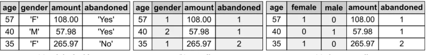
Most data transformation between SQL and ML systems deals with categorical variables. This is because categorical variables are usually represented as string fields in SQL systems, but it is very hard and inefficient to handle string values in analytics. As a result, most ML systems prefer handling numeric values only. One of the most common data transformation, therefore, is recoding of cate-gorical variables [5]. Figure 1(b) shows an example recoding of the categorical fieldsgenderandabandonedin the table shown in Figure 1(a) (This table could be the result of a query in a SQL sys-tem). The recoded numeric values are usually consecutive integers starting from 1. Here, for the fieldgender, the value ‘F’ is re-coded to 1 and ‘M’ is rere-coded to 2. And for the fieldabandoned, ‘Yes’ and ‘No’ are recoded to 1 and 2 respectively.
The above recoding is seemingly simple. In a centralized envi-ronment, it only requires one pass of data to perform the recoding of all categorical fields, assuming the number of distinct values for each field is not large. This centralized algorithm simply keeps track of a running map of current recoded values for each categor-ical field while scanning through the data. If a value of a field has been seen before, it just uses the map to recode it, otherwise a new recoding is added to the map.
In a distributed environment, however, a two-phase approach is needed. In the first phase, each local worker computes its distinct values for each categorical field in its local partition, and then ex-changes the local lists to obtain the global distinct values. In the second pass of the data, we can use the global distinct values to perform the recoding.
This two pass algorithms can be easily implemented using a combination of UDFs and SQL statements. For example, in the first pass, we can implement a parallel table UDF, which in paral-lel reads its local partition of the table and generate another table with two fieldscolName and colVal, which contains the lo-cal unique values for each categorilo-cal column. For example, the returned records in a local partition might be{(‘gender’, ‘F’),
(‘gender’, ‘M’), (‘abandoned’, ‘Yes’)}. These records can then
be passed to aSELECT DISTINCT colName, colValue FROM ...
state-ment to compute the global unique values. We can also introduce another table UDF to add a recoded value fieldrecodeValto the results, generating recode mapping records like{(‘gender’, ‘F’, 1), (‘gender’, ‘M’, 2), (‘abandoned’, ‘Yes’, 1), (‘abandoned’,
‘No’, 2)}. Let’s denote the original table asTand the recode map
table asM, then the final recoding in the second pass can be simply implemented by a join like below:
age gender amount abandoned 57 'F' 108.00 'Yes' 40 'M' 57.98 'Yes' 35 'F' 265.97 'No'
(a) original table
age gender amount abandoned
57 1 108.00 1
40 2 57.98 1
35 1 265.97 2
(b) recoding
age female male amount abandoned
57 1 0 108.00 1
40 0 1 57.98 1
35 1 0 265.97 2
(c) dummy coding
Figure 1: Recoding and dummy coding of categorical variables
SELECT T.age, Mg.recodeVal as gender, T.mount, Ma.recodeVal as abandoned
FROM T, M as Mg, M as Ma
WHERE Mg.colName=‘gender’ AND T.gender=Mg.colVal AND Ma.colName=‘abandoned’ AND T.abandoned=Ma.colVal
Although one could use SQL queries to compute the distinct val-ues, each column that needs to be recoded would result in such an SQL query, and would require one pass of the data. Using UDFs, we can scan the data once and compute the distinct values for all required columns.
Note that although categorical values are represented as strings in tables, some modern column stores are able to exploit dictionary compression to physically store string values as integers. Utiliz-ing these integers directly as the recoded values for ML systems is an interesting direction. However, there are a number of chal-lenges. First of all, the internal physical dictionary encoding is usually not exposed to users, thus utilizing the encoded integers is difficult or even impossible in a general approach using UDFs. Sec-ond, most dictionary compression for big SQL systems, such as in the Parquet format [18] for Impala and ORC format [17] for Hive, is applied only for a local partition of data. Therefore, we can-not directly use the local encoded integers for the global recoding. Lastly, some ML systems, such as SystemML [9], require the re-coded categorical values to be consecutive integers starting from 1. Some dictinary compression algorithms may not produce consecu-tive integers. Moreover, the recoding needs to be done on filtered data, and hence we may have to recode the values again.
2.2 Dummy Coding
Some ML algorithms, such as SVM and logistic regression, re-quire generating binary features from a categorical variable before invoking the algorithms. This transformation is called dummy cod-ing [4]. People also call it one-hot encodcod-ing or one-of-K encodcod-ing. Figure 1(c) shows an example dummy coding for thegenderfield in the recoded table of Figure 1(b). In dummy coding, a categori-cal variable withKdistinct values is split intoKbinary variables.
Assuming the categorical variable has already been recoded, then the original variable with valueiresults in theithbinary variable
to be 1, and the remainingK 1variables to be 0.
To implement dummy coding in big SQL systems, we only need a parallel table UDF that takes in the number of distinct values for each categorical variable (already obtained during recoding phase) and scans through each partition to perform the dummy coding in parallel.
3. PARALLEL STREAMING DATA
TRANS-FER
In this section, we describe our approach to parallel streaming data transfer. There are two main goals that we want to achieve when designing the streaming data transfer method: (1) generality of the approach on various big SQL and big ML systems, and (2) exploitation of the massive parallelism between the two systems.
SQL Worker 1 SQL Worker 2 ML Worker 2 ML Worker 3 ML Worker 4 ML Worker 1 Coordinator SQL_IP1 SQL_IP2 ML_IP1 ML_IP2 ML_IP3 ML_IP4 ML Job (1) r egis ter (2) launch (3) inp ut splits (4) re gis ter (5) match making (6) ML w orke rs to conn ect (6) S Q L w orke r to c on ne ct (7) establish connection (8) data transfer
Figure 2: Information and data flow in parallel streaming data transfer
To achieve generality, we again exploit the UDF extensibility in the big SQL systems and extend the Hadoop’s InputFormat interface in the big ML systems. In fact, most existing big ML systems [9, 1, 20] can input data through the InputFormat interface. So, a user can choose any of the existing big ML system to run the analytics. The only change she has to make is to use our specialized SQLStream-InputFormat in the job configuration. To exploit the massive paral-lelism between two independent distributed systems, we introduce a long standingcoordinatorservice to help bridge the two systems to establish parallel communication channels. In addition, we try to take advantage of data locality as much as possible when the big SQL and big ML systems share the same cluster resources.
Figure 2 shows the detailed information and data flow in our parallel data streaming method. The data transfer starts from the parallel table UDF in the SQL system. This UDF takes in as inputs the table to be transferred, the IP and port number of the coordina-tor, as well as the command and arguments to invoke the desired algorithm of the target ML system. When this UDF is executed in each SQL worker, it first connects to the coordinator, notifies the coordinator of its own worker id, IP address, and the total number of active SQL workers, and also passes along the command and ar-guments of the target ML algorithm (step 1 in Figure 2). When all the SQL workers have registered, the coordinator launches the ML job with the provided command and arguments (step 2).
When the ML job tries to spawn tasks to read data, it first creates an InputFormat object. InputFormat has a member function called getInputSplits(), which is responsible for dividing the input data into subsets. Each subset is called an InputSplit and is consumed by one ML worker. In other words, the number of InputSplits equals
to the number of ML workers. We customized the getInputSplits method to contact the coordinator to decide on the InputSplits (step 3). Letnbe the number of SQL workers andmbe the number of InputSplits. Ifmis not pre-specified by the particular ML
al-gorithm, then we always setm=n⇥k, wherekis a parameter to control the degree of parallelism in the ML job. We divide the neededmInputSplits evenly intongroups, with each group
cor-responding to the data from one SQL worker, as demonstrated in Figure 2. To take advantage of the potential locality, we also pro-vide the locations for each InputSplit where the data for the split would be local. In particular, for each InputSplit corresponding to theithSQL worker, we use the IP address of this SQL worker as
the location of the InputSplit. With the provided locations, when the ML job spawns the ML workers to read data, it tries to colo-cate, when possible, in a best effort manner, the ML workers with the corresponding SQL workers, so that data transfer does not incur network I/O.
After the ML workers are spawned, they register themselves back to the coordinator (step 4 in Figure 2). Then, the coordinator matches the IP of each SQL worker with the IPs of its correspond-ing ML workers (step 5), and subsequently sends the matched in-formation back to the workers on both sides (step 6). Now, the job of the coordinator is done. Finally, the SQL workers and the ML workers establish the TCP socket connections (step 7), before the actual data transfer starts (step 8). Each SQL worker sends data to its ML workers in a round robin fashion. Inside a SQL worker, there is a send-buffer associated with each target ML worker for buffering the sent data. Similarly, each ML worker has a receive-buffer to receive-buffer the received data from its corresponding SQL worker. The sizes of the buffers are controllable system parameters. If an ML worker is slow to ingest its data and the corresponding send buffer becomes full, we can spill it onto the local disks to syn-cronize the producer and consumers.
4. QUERY REWRITER FOR DATA
TRANS-FORMATION AND TRANSFER
Although we have provided various UDFs for the common data transformation and parallel data streaming, it is still a difficult task for the users to compose the queries to invoke these UDFs. For ease of use, we provide a query rewriter outside the SQL systems. A user provides this query rewriter with her SQL query (such as the example query in Section 1), the transformations needed on the results of the query, and if parallel data streaming is needed, the necessary information for calling the target ML algorithm. Then, the query rewriter will extend the given query into another query with UDFs, and other operations to perform the required transfor-mations and the data transfer.
5. CACHING
When similar data transformations are repeated between a big SQL system and a big ML system, we can exploit caching to reduce the cost. We identified two cases of caching, assuming there is no data update: (1) caching fully transformed data, and (2) caching intermediate recode maps.
5.1 Caching Fully Transformed Data
In this case, we cache the fully transformed data in the big SQL system by storing it as a materialized view or an actual HDFS table. If later another ML algorithm needs to be run on the data resulted from the same SQL queries, we can directly reuse the stored data, thus saving the cost of the SQL queries and the data transformation all together. This situation happens, for example, when an analyst
wants to run a number of classification algorithms, such as SVM, logistic regression, naive Bayes and decision trees, to compare the quality of different classifiers on a particular dataset.
Besides the above case, the fully transformed data can also be reused if a subset of the transformed data is needed. Let’s take the example scenario in Section 1 as an instance. If we cache the fully transformed result of this query, and later we encounter another query shown below as the data preparation for an ML algorithm, we can fully utilize the cached data, without running the query and transforming the query result.
SELECT U.age, C.amount, C.abandoned FROM carts C, users U
WHERE C.userid=U.userid AND U.country=‘USA’ AND U.gender = ‘F’
The reason that we can fully utilize the cached result is that this new query satisfy the following conditions:
1. It contains the same tables in the from clause, and the same join conditions and predicates in the where clause, as the query for the cached data.
2. The projected fields are a subset of the projected fields in the query for the cached data.
3. Additional conjunctive predicates are only on the projected fields in the query for the cached data.
In fact, if we denote the result of query in Section 1 asT, the new query can be expressed as a selection and projection query on table
Tas below.
SELECT age, amount, abandoned FROM T
WHERE gender = ‘F’
5.2 Caching Recode Maps
The applicability of caching the fully transformed data is limited. For the following query, the cached data cannot be used at all, as it does not satisfy the conditions described in the previous subsec-tion.
SELECT U.age, U.gender, C.amount, C.nItems, C.abandoned FROM carts C, users U
WHERE C.userid=U.userid AND U.country=‘USA’ AND C.year = 2014
However, we notice that this query satisfies a different set of con-ditions, which allow it to benefit from caching the intermediate re-code map (see Section 2.1) generated during the transformation of the previous query:
1. It contains the same tables in the from clause, and the same join conditions in the where clause, as the previous query. 2. It contains predicates on the same set of fields as the
pred-icates on the previous queries, and each predicate is either the same as or logically stronger than (e.g. a <18is
log-ically stronger thana20) the corresponding predicate in the previous query.
3. The projected categorical fields are a subset of the projected categorical fields in the previous query.
4. Additional predicates are conjunctive.
By reusing the recode map for the new query, we avoid one of the two passes for the new query during recoding.
As can be seen above, the way we detect whether a query can benefit from the cached data is similar to utilizing materialized
views in query optimization [10, 16] and we extend the query rewriter introduced in Section 4 to utilize these techniques. When the rewriter gets a query, it first check to see if any of the existing materialized views can be used and rewrites the query accordingly.
6. DISCUSSION ON FAULT TOLERANCE
Fault tolerance is a very hard problem for integrating big SQL and big ML systems. First of all, if either the underlying big SQL system or the big ML system lacks fault tolerance support, the whole integration pipeline has to be restarted from scratch in case of a failure. In fact, most MPP databases do not support mid-query failure recovery. Most SQL-on-Hadoop engines, like Impala [14] also sacrifice mid-query recory. As for big ML systems, MLlib is the only one known to support mid-query fault tolerance. Even both underlying systems provide fault tolerance guarantees, we still need the connection between the two to be resilient to failures. If data transfer between the two systems is through files on HDFS, or if the cached results from the big SQL system can be directly reused by the big ML system, the fault tolerance can be guaranteed. On the other hand, if parallel data streaming in Section 3 is used, more care has to be taken. First, we need the coordinator service to be resilient itself. This can be achieved by using Zookeeper [2]. In addition, when the data transfer between a SQL worker and an ML worker fails, due to the failure of either end points or the connection, we need to notify the big SQL system to restart the SQL worker and simultaneously tell the big ML system to restart all the ML workers corresponding to the SQL worker, so that the data transfer can be resumed.
An alternative to our streaming data transfer is utilizing an in-memory file system like Tachyon [15], which would provide fault-tolerance guarantees. However, Tachyon is still very Spark and RDD oriented, whereas in this work we thrive to be provide a generic solution that works for all big SQL and big ML systems, whether they run their own native processes, or use MapReduce or Spark.
7. PRELIMINARY EXPERIMENTS
In this section, we report the results of our preliminary experi-mental study by using IBM Big SQL 3.0 as the big SQL system and Spark MLlib as the big ML system.
We used 5 servers for all our experiments. Each had 2x Intel Xeon CPUs @ 2.20GHz, with 6x physical cores each (12 phys-ical cores in total), 12x SATA disks, 1x 10 Gbit Ethernet card, and a total of 96GB RAM. Each node runs 64-bit Ubuntu Linux 12.04, with a Linux Kernel version 3.2.0-23. One of the servers was used as the HDFS NameNode, MapReduce JobTracker, Spark master as well as Big SQL head node. The remaining 4 servers host the HDFS DataNodes, MapReduce TaskTrackers (9 mappers per server), Spark workers (6 workers on each server) and Big SQL workers (1 worker with multi-threading on each server). HDFS replication was set to 3. The send-buffer and receive-buffer sizes were both set to 4KB for the parallel data streaming.
We generated synthetic datasets in the context of the example query scenario described in Section 1. In particular, we created a 56GB carts table with 1 billion records and 361 MB users table with 10 million records. Both tables were stored in text format on HDFS. We ran the SQL query shown in the example in Sec-tion 1, transformed the result (recoding the categorical variables and dummy coding), and passed the result to MLlib for running the SVMWithSGD algorithm. In our experiments, we report the time for processing the SQL query, transforming the result, transferring the transformed data to the ML job, and reading the input data in
0 200 400 600 800 1000 1200
naïve insql insql+stream
ti m e (s e c ) input for ml trsfm prep prepl+trsfm prep+trsfm+input
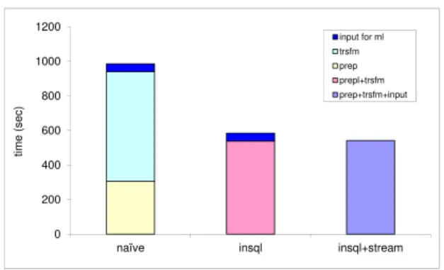
Figure 3: Comparison of three approaches of connecting big SQL and big ML systems
0 100 200 300 400 500 600
no cache cache recode maps cache transformed result ti m e ( s e c )
Figure 4: Effect of caching
the ML job. We do not report the runtime of the ML algorithm, because it is highly dependent on the actual data and the algorithm (e.g how many iterations to converge). For example, reading the transformed data from HDFS and running the SVMWithSGD for 10 iterations took 774 seconds. In the ML job, we first read the input data, whether it is from HDFS or from parallel data transfer, into a Spark in-memory RDD. After that we pass the RDD to the MLlib SVMWithSGD algorithm. The measured time of reading input in the ML job is the time from the start of the job till the in-memory RDD is constructed.
Figure 3 compares three approaches of connecting SQL with ML for big data. In the naive (denoted as naive in Figure 3) approach, we use Big SQL to execute the SQL query and materialize the re-sult on HDFS (prep). Then, we use a third tool, Jaql [3], to perform the data transformation, since Jaql has built-in functions for recod-ing of categorical variables and dummy codrecod-ing (trsfm). Again, the result is written to HDFS. Finally, Spark MLlib reads the data form HDFS (input for ml) and performs the ML job. The breakdown of execution times for different stages is shown in the figure. The sec-ond approach, denoted as insql in the figure, employs the In-SQL transformation method (we implemented the recoding of categor-ical variables and dummy coding in Big SQL using UDFs). In this approach, the transformation is combined together with the SQL query, thus the operations can be performed in a pipeline (prep+trsfm). In the third approach, denoted as insql+stream, we
use the parallel streaming data transfer in addition to the In-SQL transformation. Now, all operations can be pipelined together (prep +trsfm+input). In addition, as we use in-memory RDDs to store the input data in Spark for the ML job, the transformed data from Big SQL is never written to HDFS. As can be seen from Figure 3, the In-SQL transformation significantly improves the performance of the whole work flow: 1.7x speed up against the naive approach. The insql+stream approach further improves the performance by another 43 seconds. This is a significant reduction in data inges-tion cost in Spark MLlib (reading from HDFS takes 46 seconds), although it is not an impressive number in the overall workflow. In this particular case, the transformed data itself was not very large (5.6GB), and hence reading it from HDFS was not dominating the overall data pipeline. If a larger dataset were used, the performance would be more dramatic. We also want to note that if the ML algo-rithm takes a long time to produce the desired model, then whether using HDFS or streaming for data transfer makes little difference in the overall performance. In addition, HDFS can also provide ad-ditional fault tolerance, and could be preferable if the ML system requires reading the input multiple times.
We now investigate the effect of caching intermediate or final results of data transformation in connecting big SQL and big ML systems. We compare the In-SQL transformation approach with the approach where we cache intermediate recode maps, and the approach where we cache the fully transformed result in Figure 4. In all three approaches, we employ the parallel streaming trans-fer to pass data to the ML job. Evidently, if caching can be used, then the fully cached result will provide the best performance (2.2x speedup against no cache), followed by the cached intermediate re-code maps (1.5x speedup against no cache). But, keep in mind that the applicabilities of the two caching approaches are limited, with caching the fully transformed result most limited. For both caching methods, the reusability depends on the complexity of the prepara-tion SQL query and how fast, or if at all, the data gets updated.
8. CONCLUSION
In this paper, we studied the problem of integrating SQL and ML processing for big data, providing a general purpose solution that will work withanybig SQL system that supports UDFs andanybig ML system that uses InputFormats to ingest its input. We focused on two problems: data transformation and data transfer between the two systems. In particular, we proposed an In-SQL approach to in-corporate common data transformations for ML algorithms inside big SQL systems through UDFs. In addition to the basic approach of using files as the media for data transfer between systems, we proposed a general streaming data transfer approach by introduc-ing UDFs in big SQL systems and implementintroduc-ing a special Hadoop InputFormat. Furthermore, we explored the use of caching inter-mediate or final results of the transformations to reduce the costs of connecting SQL and ML systems. Our preliminary experimental results show that the In-SQL approach has great potential in reduc-ing the data transformation cost, and cachreduc-ing is very effective in improving the performance of the whole analytics work flow. The parallel streaming data transfer approach has its pros and cons, de-pending on the target ML system. Our preliminary experiments show it results in significant reduction in data ingestion costs for MlLib, which uses in-memory RDDs.
As future work, we plan to investigate using a message passing system like Kafka [8] to pass the data between SQL and ML work-ers. Kafka would gurantee at least one read, in case of failures. Kafka could also be the system to cache the data when the ML workers are not fast enough to consume the data. We also plan to build a generic data exchange infrastructure that utilizes memory
and streaming between different frameworks running on big data platforms, such as streaming, batch, SQL, ML, etc.
9. REFERENCES
[1] Apache Mahout.https://mahout.apache.org. [2] Apache ZooKeeper.
http://zookeeper.apache.org.
[3] K. S. Beyer, V. Ercegovac, R. Gemulla, A. Balmin, M. Y. Eltabakh, C.-C. Kanne, F. Özcan, and E. J. Shekita. Jaql: A scripting language for large scale semistructured data analysis.PVLDB, 4(12):1272–1283, 2011.
[4] D. Conway and J. M. White.Machine Learning for Hackers. O’Reilly Media, 2 2012.
[5] Cookbook for R: Recoding data.
http://www.cookbook-r.com/Manipulating_ data/Recoding_data.
[6] Dummy, effect, & orthogonal coding.
http://luna.cas.usf.edu/~mbrannic/files/ regression/anova1.html.
[7] X. Feng, A. Kumar, B. Recht, and C. Ré. Towards a unified architecture for in-rdbms analytics. InSIGMOD, pages 325–336, 2012.
[8] R. C. Fernandez, P. Pietzuch, J. Koshy, J. Kreps, D. Lin, N. Narkhede, J. Rao, C. Riccomini, and G. Wang. Liquid: Unifying Nearline and Offline Big Data Integration. In
CIDR, 2015.
[9] A. Ghoting, R. Krishnamurthy, E. Pednault, B. Reinwald, V. Sindhwani, S. Tatikonda, Y. Tian, and S. Vaithyanathan. SystemML: Declarative machine learning on mapreduce. In
ICDE, pages 231–242, 2011.
[10] A. Y. Halevy. Answering queries using views: A survey.The VLDB Journal, 10(4):270–294, 2001.
[11] J. M. Hellerstein, C. Ré, F. Schoppmann, D. Z. Wang, E. Fratkin, A. Gorajek, K. S. Ng, C. Welton, X. Feng, K. Li, and A. Kumar. The madlib analytics library: Or mad skills, the sql.PVLDB, 5(12):1700–1711, 2012.
[12] Hivemall.https://github.com/myui/hivemall. [13] IBM Big SQL 3.0: Sql-on-hadoop without compromise.
http://public.dhe.ibm.com/common/ssi/ ecm/en/sww14019usen/SWW14019USEN.PDF. [14] Impala.http://github.com/cloudera/impala. [15] H. Li, A. Ghodsi, M. Zaharia, S. Shenker, and I. Stoica.
Tachyon: Reliable, Memory Speed Storage for Cluster Computing Frameworks. InSOCC, 2014.
[16] I. Mami and Z. Bellahsene. A survey of view selection methods.SIGMOD Rec., 41(1):20–29, 2012.
[17] The ORC format.http:
//docs.hortonworks.com/HDPDocuments/ HDP2/HDP-2.0.0.2/ds_Hive/orcfile.html. [18] The Parquet format.http://parquet.io.
[19] R.http://http://www.r-project.org/. [20] Spark MLlib.https://spark.apache.org/mllib. [21] A. Thusoo, J. S. Sarma, N. Jain, Z. Shao, P. Chakka,
S. Anthony, H. Liu, P. Wyckoff, and R. Murthy. Hive: A warehousing solution over a map-reduce framework.
PVLDB, 2(2):1626–1629, 2009.
[22] How-to: Use MADlib pre-built analytic functions with impala.
http://blog.cloudera.com/blog/2013/10/
how-to-use-madlib-pre-built-analytic-functions -with-impala.